Feature Selection with Optimal Variational Auto Encoder for Financial Crisis Prediction

1  Introduction

With the growth in financial crises affecting businesses all over the world, researchers have been paying close attention to the domains of financial crisis prediction (FCP) [1]. It is critical for a financial or business institute to develop an earlier and more reliable forecasting strategy for predicting the likelihood of a company’s financial demise. As market competition becomes more robust, the risk of a monetary crisis for freely traded enterprises is continuously increasing [2]. The most pressing issue among creditors, operators, and other stakeholders of listed firms, as well as investors, is whether they can correctly foresee the economic catastrophe.

Economic crisis estimation entails a review of a company’s financial reports, commercial plans, and other related accounting resources, as well as the application of accounts, comparative analysis, statistics, finance, institution management, factor analysis, and other analysis procedures to quickly address issues identified in the company [3]. Furthermore, economic crisis estimation entails the development of associated models based on monetary pointers that accurately and broadly describe the economic situation of industries, followed by the use of the ideal to predict the likelihood of an economic crisis [4].

FCP often produces a binary classification algorithm that has been rationally resolved [5]. The company’s failure and non-failure status are determined by the classification system [6]. An additional number of classifiers have been advanced using various field information for FCP. Commonly, existing estimation techniques can be divided into statistical methods or artificial intelligence methods (AI). Higher dimensional data, particularly in terms of distinct features, is becoming more prevalent in machine learning (ML) difficulties. The majority of the researchers concentrated on the study in order to tackle the problems [7]. Also, to extract significant attributes from these high-dimensional variables and data. To eliminate redundant data and noise, statistical models were used. As a result, feature selection (FS) plays an important role in developing our model with correlated and non-redundant attributes [8]. When clearing the redundant one, the original attribute is reduced to a smaller one, preserving the required information, and it is indicated as FS. In order to fix these issues, we need to use fewer training instances. These situations would be notable for their use of FS and feature extraction approaches. The FS approach is widely used to boost a classification’s generalization ability. FS methodology is frequently employed to surge the generalization potential of a classification.

Recently, the AI technique is proposed to refine traditional classification techniques, even though the existence of different features in the high dimensional monetary information is the reason for several challenges, such as over-fitting, low interoperability, and high computational difficulty. The dimensionality curse describes how many samples are required to create a random function with an accuracy level that grows exponentially with the number of inputs [9]. The easiest way to solve the problem is minimalizing the present feature count with the help of FS technology. The FS approach focuses on recognizing appropriate feature subsets and has crucial inference for problems, such as (i) cost consumption and computational time required to develop an appropriate method, (ii) reducing noise by removing noisy features, (iii) enabling easy access setting and updating technique, and (iv) reorganization resulting technique. The selected set of features is applicable for representing classification function that influences various dimensions of classification namely cost cohesive with features, learning duration, and the accuracy of the classifier technique. The FS technique is used in a variety of applications, including data mining, pattern recognition, and machine learning, to improve classification prediction accuracy and reduce feature space dimensionality. According to the evaluation standards, the FS method is spitted into the wrapper-, filter-, and embedded-based approaches. The wrapper approach applies a learning model as an assessment part to measure the advantages of the feature set. The wrapper technique, on the other hand, has less drawbacks, such as identifying the learner’s user-defined parameter, intrinsic learner restriction, and maximum computing complexity [10]. When compared to the wrapper approach, the embedded strategy is easier to calculate; however, the selected collection of characteristics is useless in the learning procedure. Because of this limitation, the filter method is used in various techniques.

The authors of [11] focus on mid-and long-term bankruptcy predictions (up to sixty months) for small and medium-sized businesses. A significant impact of these cases is the significant improvement in forecast accuracy from the short-term (12 months) using ML techniques, as well as the creation of accurate mid-and long-term projections. The authors of [12] looked at the likelihood of bankruptcy for 7795 Italian municipalities from 2009 to 2016. Because there were so few bankruptcy instances to learn from, the forecasting process was extremely difficult. Furthermore, historical financial data for all municipalities, as well as socioeconomic and demographic circumstances, can be used as alternative institutional data. The predictabilities were examined with the efficiency of the statistical and ML techniques with receiver operating characteristic (ROC) and precision-recall curves.

In [13], the random forest (RF) technique inspired expert voting procedure is the more efficient classification demonstrating comparatively higher generalization above 80% AUC curve on creating the early warning system (EWS). In contrast, the convention scheme, a visual representation of evidence, shows that the expert voting EWS synthesis multi-variate data is suited for providing systemic banking systemic crises alerts in many circumstances. In [14], the authors compare the effectiveness of the ML boosting techniques CatBoost and extreme gradient boosting (XGBoost) with the usual approach of credit risk assessment, logistic regression (LR). While grid search is used, both strategies are applied to two different datasets. In [15], the authors investigate a novel FS for FCP that combines elephant herd optimization (EHO) with a modified water wave optimization (MWWO) technique based deep belief network (DBN). The MWWO-DBN technique was used for the classifier procedure, and the described technique was used as a feature selector. The usage of the MWWO technique aids in the tuning of the DBN technique’s parameters, while the EHO technique’s selection of the best feature subset improves classifier efficiency.

Sankhwar et al. [16] establish a new prediction structure for the FCP method by incorporating a fuzzy neural classifier (FNC) and improved grey wolf optimization (IGWO). An IGWO technique was resultant from the combination of the grey wolf optimizer (GWO) technique and tumbling effects. The projected method based FS technique was utilized for discovering the optimum feature in the financial information. FNC was used to classify the results. FNC was used to classify the results. Ma et al. [17] examined an enhanced ML technique and called it machine learning in information access (MLIA) technique. Meanwhile, this investigation breaks down the goal function into weight sums of numerous fundamental functions. It is possible to compare the efficacy of MLIA predictive technique and logistic predictive technique using three traditional test functions. In addition, the study looks at the performance of the MLIA financial credit risk forecasting approach using data from Internet financial organisations.

The goal of Liang et al. [18] is to analyse the predictive efficiency achieved by combining seven different types of financial ratios (FRs) and five different types of corporate governance indicators (CGIs). The experimental results based on a real-world data set in Taiwan showed that one of the main elements of bankruptcy prediction is the FR category of solvencies and profitability, as well as the CGI categories of board infrastructure and ownership infrastructure. Uthayakumar et al. [19] present an Ant Colony Optimization (ACO) based FCP technique that integrates 2 stages: ACO based feature selection (ACO-FS) technique and ACO based data classification (ACO-DC) technique. The proposed technique was validated utilizing a group of 5 standard datasets containing both quantitative as well as qualitative. In order to FS designs, the established ACO-FS approach was related to 3 presented FS techniques such as genetic algorithm (GA), particle swarm optimization (PSO), and GWO technique.

This study presents a novel multi-vs. optimization (MVO) based feature selection (FS) model for FCP that uses an optimum variational auto encoder (OVAE). The article explains why this model is used and also proposes a novel multi-vs. optimization (MVO) based feature selection (FS) for FCP using an optimal variational auto encoder (OVAE) model. The suggested MVOFS-OVAE model uses min-max normalization to pre-process the financial data. In addition, the MVOFS-OVAE model employs the MVOFS technique to create a feature subset selection procedure. Followed by, the VAE model is applied for the categorization of financial data into financial crises or non-financial crises. Finally, the VAE method’s parameters are tuned using the differential evolution (DE) technique. As a result, the MVOFS technique is primarily used to pick ideal features, while the DE algorithm is used to select optimal VAE model parameters. The MVOFS-OVAE strategy outperformed the latest state-of-the-art approaches in a series of simulations on the standard dataset.

2  Materials and Methods

In this study, a novel MVOFS-OVAE model was established to accomplish forecasting the financial crisis. The MVOFS-OVAE model encompasses a series of operations such as min-max normalization, MVO based feature subset selection, VAE based classifier, and DE based parameter optimization. Fig. 1 depicts the overall process of the MVOFS-OVAE approach. The working process of these modules is discussed in the following.

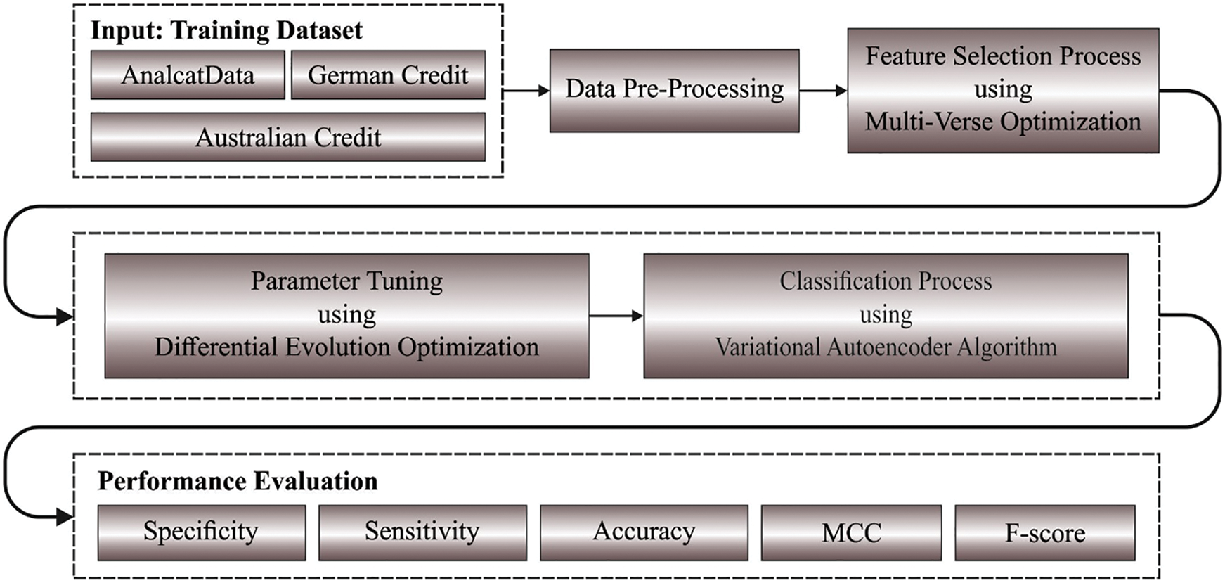
Figure 1: Overall Process of MVOFS-OVAE technique

2.1 Algorithmic Design of MVOFS Technique

The MVOFS technique is used to choose the best feature subsets in this research. The MVO approach is a crucial simulation of the multiverse model established from astrophysics. Mirjalili et al. [20] stated that MVO matter is moved from one universe to another via white or black holes, which appeal and emit matter in the same way. Wormholes connect universes on opposite sides. The following are key words in this model: all universes are solutions, but all solutions are included in a series of objects, generations, or iterations that are used to show time, and the inflation rate was used to show the value of all the objects from a single universe.

xi′={xkjr1<NI(Ui)xijr1≥NI(Ui) (1)

whereas Xij signifies the jth object of the ith universe, r1 refers to the arbitrary number from an existing spectrum ranging in [0–1], NI (Ui) is equivalent to the normalizing inflation rate of the ith universe and Xkj defines the jth object of kth universe.

xij={xj+TDR×((Ubjb−Lbjb)×r4×Lbjb)ifr3<0.5andr2<WEP,xj−TDR×((Ubjb−Lbjb)×r4×Lbjb)ifr3≥0.5andr2<WEP,xijifr2≥WEP, (2)

In which Xj is the jth centroid of an optimum universe attained so far, UB signifies the upper bound, LB equivalents the minimal bound, Traveling Distance Rate (TDR) and Wormhole Existence Probability (WEP) are co-efficient, r2, r3 , and r4 demonstrates the arbitrary values ranging in [0–1]. In addition, this technique of MVO signifies the ideal solution for optimizing and executing it for influencing other solutions. During the original research, the authors maintained that wormholes are established in every universe. Again, in turn, it improves the probability of containing access to optimum solutions and maintained the ideal solution that is attained from the optimized procedure. In the final optimization, the ideal solution was attained as a global optimal to specific problems. The MVO has of the succeeding procedure to suitable concentration on distinct patterns under the optimized patterns that are as follows:

WEP=Min+Iteration×(Max−MinL) (3)

TDR=1−Iteration1/pL1/p (4)

whereas p signifies the exploitation element.

The MVO purposes for discovering the optimum feature subset for an offered data set which is the superior classification accuracy and lesser features. These 2 indicators are various influences on classifier accuracy. At this point, it can be combined with a single weighted indicator and utilize the same FF as:

fitness=ω1×acc(classifier)+ω2×(1−sp), (5)

In which p characterizes the total amount of features, and s refers to the quantity of chosen features. The values of ω1 and ω2 are predefined parameters. At this point, the value of ω1 and ω2 are 1 and 0.001, correspondingly. The values ω1 and ω2 as 1 and 0.001 in such a way that the classification results can be enhanced. The acc(classifer) implies the classifier accuracy reached in the VAE classifier which is provided as:

acc(classifier)=ncnc+ni×100%. (6)

At this point, ni and nc imply the count of incorrect and accurate classification samples correspondingly. The fitness value achieves the objective which chosen feature is of maximal classification accuracy and lesser count of features.

2.2 VAE Based Classification

The VAE model is used to categorize financial data into financial crisis or non-financial crisis during the FCP process. VAE is a generating method that consists of two networks: an encoder network Q_ (ZX) and a decoder network P_ (X|Z). The gradient descent approach is used to train VAE to learn accurate inference. The encoder network with parameter learns an effective compression of the information into this low dimension space by mapping data X to a latent variable Z. The latent parameter is used by the decoder network with parameter to generate information that maps Z to recreated information X. We now use a deep neural network to build the encoder and decoder with the variables and, respectively [21]. Fig. 2 demonstrates the structure of VAE.

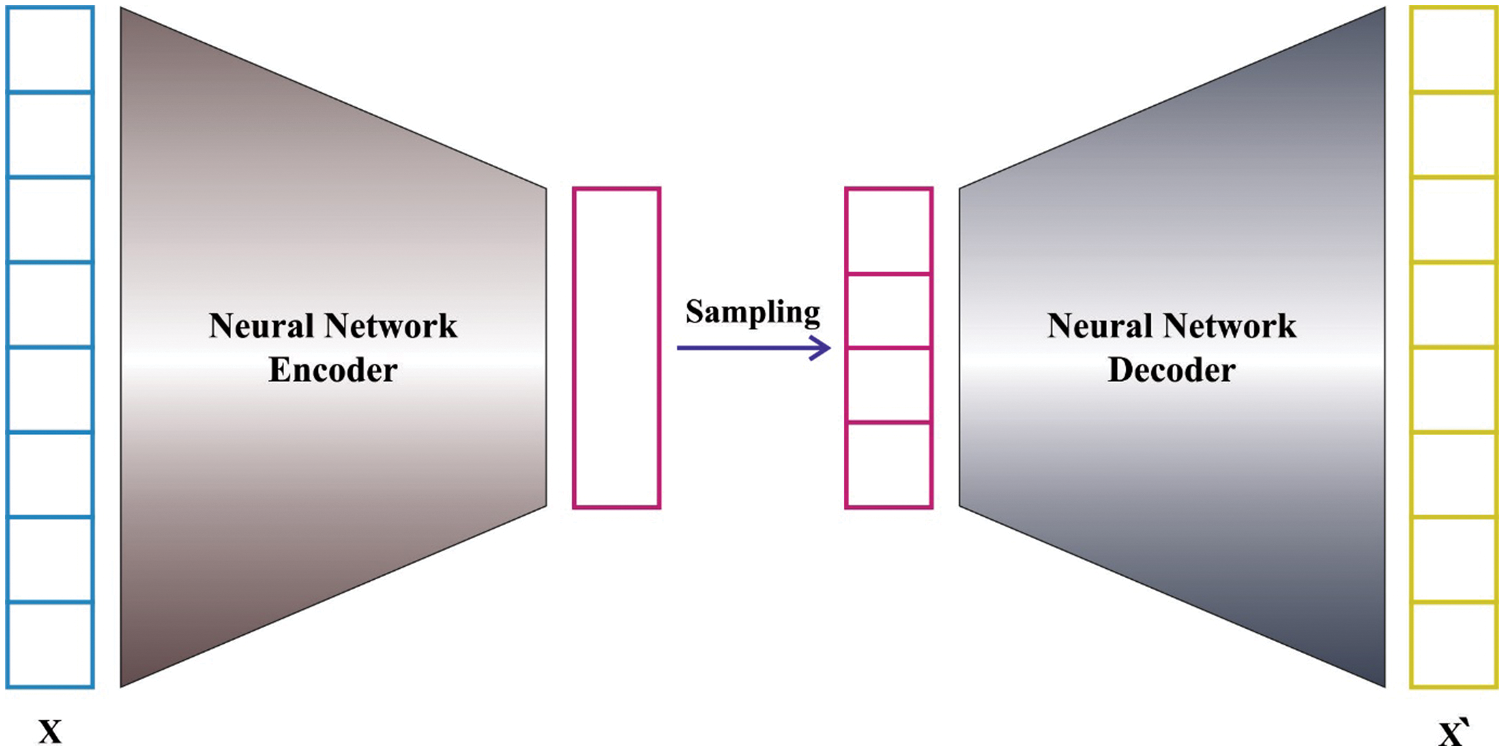
Figure 2: Variational auto encoder model

The main concept of VAE is to utilize the possibility distribution P(X) to sample data points that match the distribution, whereas X characterizes a random parameter of the data. The objective of VAE is to recreate the input dataset, viz., to exploit the log possibility of P(X) :

log⁡P(X)=E[log⁡P(X|Z)]−DKL[Q(Z|X)|P(Z)]+DKL[Q(Z|X)P(Z|X)] ≥ E[logP(X|Z)] − DKL[Q(Z|X)||P(Z)].)]. (7)

Now, the variational low bound objective [21,22] is determined by:

L(θ,φ,X)=E[logP(X|Z)] − DKL[Q(Z|X)||P(Z)]. (8)

L represent the variational lower bound that is named the VAE objective function. The initial term in Eq. (8) represents the recreation loss. This inspires the decoder to learn to recreate the input dataset. The next item in Eq. (8) employs KL (KullbackLeibler) divergence to reduce the variance among the encoder distribution Q(ZX) and the previous distribution (Z) that is to say, the learned distribution Q(ZX) is analogous to the previous distribution P(Z) [22]. Thus, the aim of training VAE is to increase the generation possibility logP(XZ) and reduce the variance between the true prior distribution (Z) and the learned distribution Q(ZX) . In another word, the aim of training VAE is to reduce the variation lower bound L.

2.3 Parameter Optimization

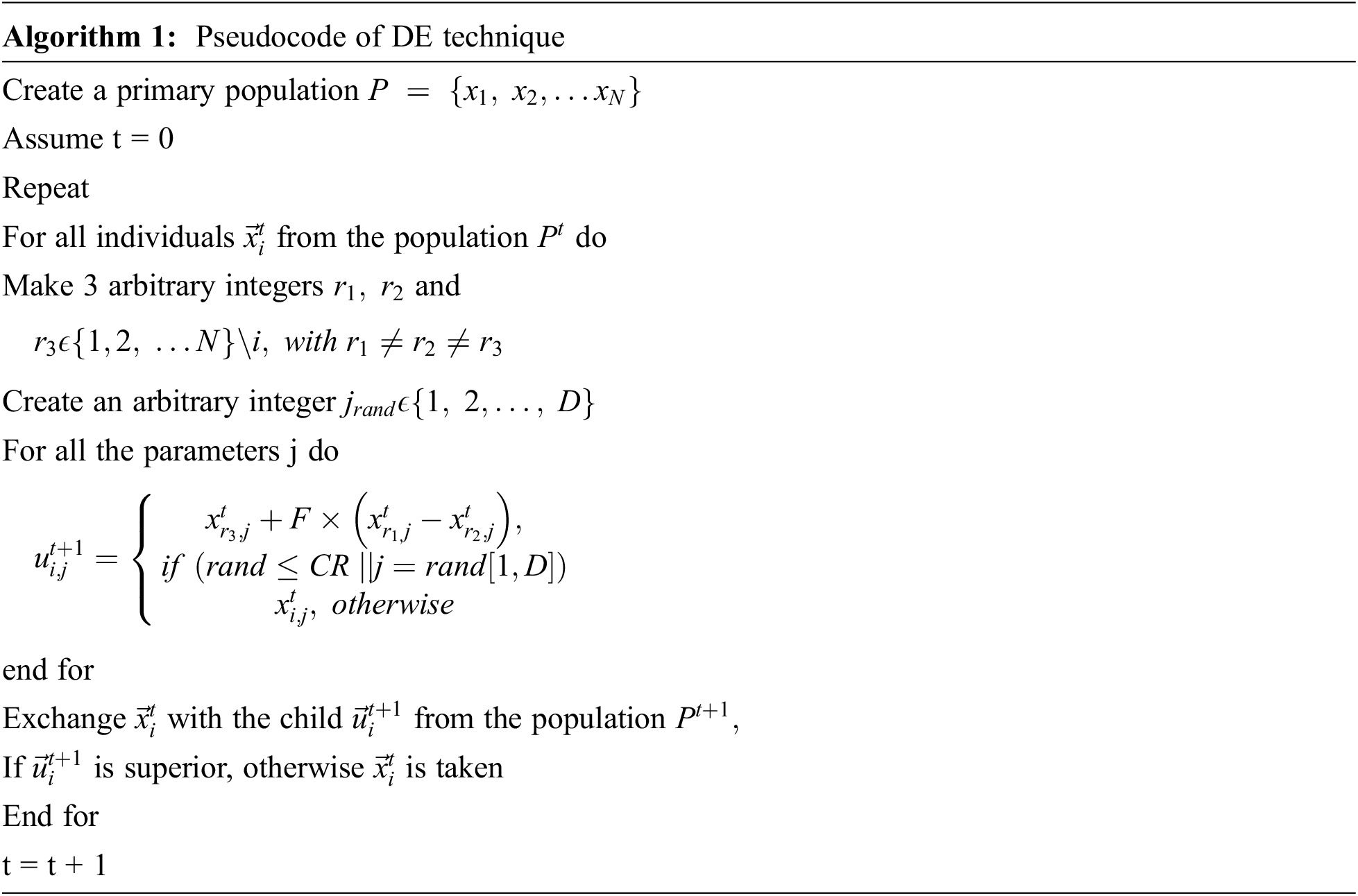
At the final stage, the DE algorithm is utilized for the parameter tuning of the VAE model. DE refers to rapid acceleration pattern, versatility quick execution time, accurate and fast local operator [23]. In DE, the optimization method initiates by randomly selecting the solution to find the majority of the points in the searching space. Then, the solution is enhanced with a sequence of operators named mutation and crossover. The novel solution is accepted when it has high objective values. For the present solution Xi , the arithmetical expression of the mutation operator Zit is given in the following:

Zi,j=XDrand1+F×(XDr2−XDr3), (9)

whereas r1,r2 , and r3 denote random numbers, F indicates the mutation balancing factor, and F is higher when compared to 0. For the crossover operator, Eq. (6) denotes the new solution Vi , which is generated by the mutated operator via the crossover Zi . The crossover is taken into account as a mixture method amongst vectors Zi and XDi.

Vi,j={Zi,jifrand≤CrXDi,jotherwise (10)

Cr denotes the crossover possibility. The DE approach enhances its selected solution based on the objective function value, in which the produced Vi, C−Iter is substituted with the existing one when it attained a good fitness value in the following.

XDi,j={Vi,jiff(Vi,j)<f(XDi,j)XDi,jotherwise (11)

The DE approach resolves a FF for obtaining superior classifier accuracy. It resolves a positive integer for characterizing the effectual accuracy of the candidate solution. In event of, the minimizing of classifier error rate was assumed as FF. An optimal solution is a lesser error rate and the least solution accomplishes an enhanced error rate.

fitness(xi)=ClassifierErrorRate(xi)=numberofmisclassifiedsamplesTotalnumberofsamples∗100 (12)

3  Performance Validation

The proposed MVOFS-OVAE model is tested using the three benchmark datasets. The details related to the dataset are given in Tab. 1.

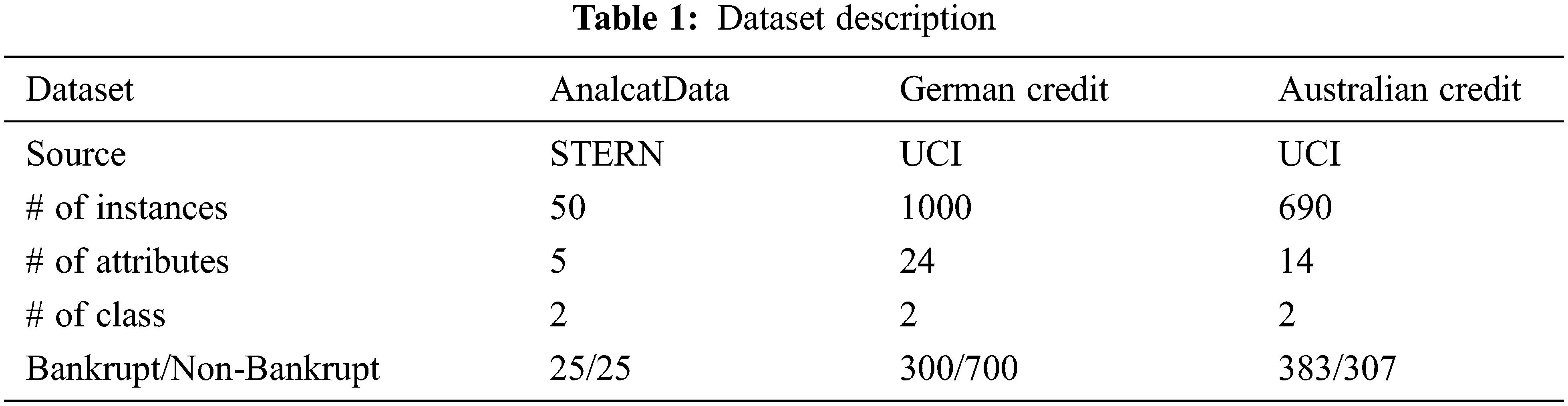
The FS outcomes of the MVOFS technique on three distinct datasets are shown in Tab. 2. On the test Analcatdata dataset, the MVOFS-OVAE model has chosen a set of 3 features. Likewise, on the test German credit data set, the MVOFS-OVAE approach has chosen a set of 14 features. Moreover, on the test Australian credit data set, the MVOFS-OVAE technique has chosen a set of 8 features.

Tab. 3 and Fig. 3 provides the best cost (BC) outcomes of the MVOFS technique with existing models on three datasets. On the Analcatdata dataset, the MVOFS model has provided a lower BC of 0.0149 while the QABO-FS, ACO-FS, and GWO-FS models have offered higher BC of 0.0149, 0.0330, and 0.0470 correspondingly.

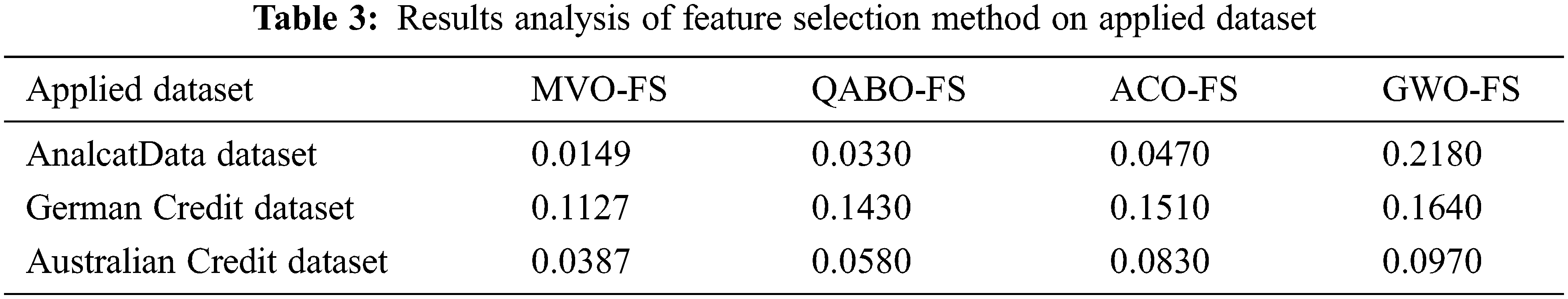
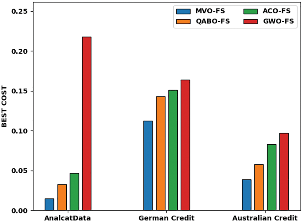
Figure 3: Average best cost analysis of different methods on applied dataset

Fig. 4 demonstrates the confusion matrices offered by the MVOFS-OVAE model on three distinct datasets. On 70% of training data on the Analcatdata dataset, the MVOFS-OVAE model has identified 18 instances of bankrupt and 14 instances of non-bankrupt classes. At the same time, on 30% of testing data on the Analcatdata dataset, the MVOFS-OVAE technique has identified 5 instances into bankrupt and 10 instances into non-bankrupt classes. In line with, 70% of training data on the German credit dataset, the MVOFS-OVAE technique has identified 188 instances of bankrupt and 475 instances into non-bankrupt classes. Moreover, on 30% of the German credit dataset testing data, the MVOFS-OVAE technique has identified 86 instances into bankrupt and 202 instances into non-bankrupt classes. Furthermore, on 70% of training data on the Australian credit dataset, the MVOFS-OVAE technique has identified 273 instances into bankrupt and 193 instances into non-bankrupt classes. At last, on 30% of testing data on the Australian credit dataset, the MVOFS-OVAE technique has identified 100 instances into bankrupt and 104 instances into non-bankrupt classes.

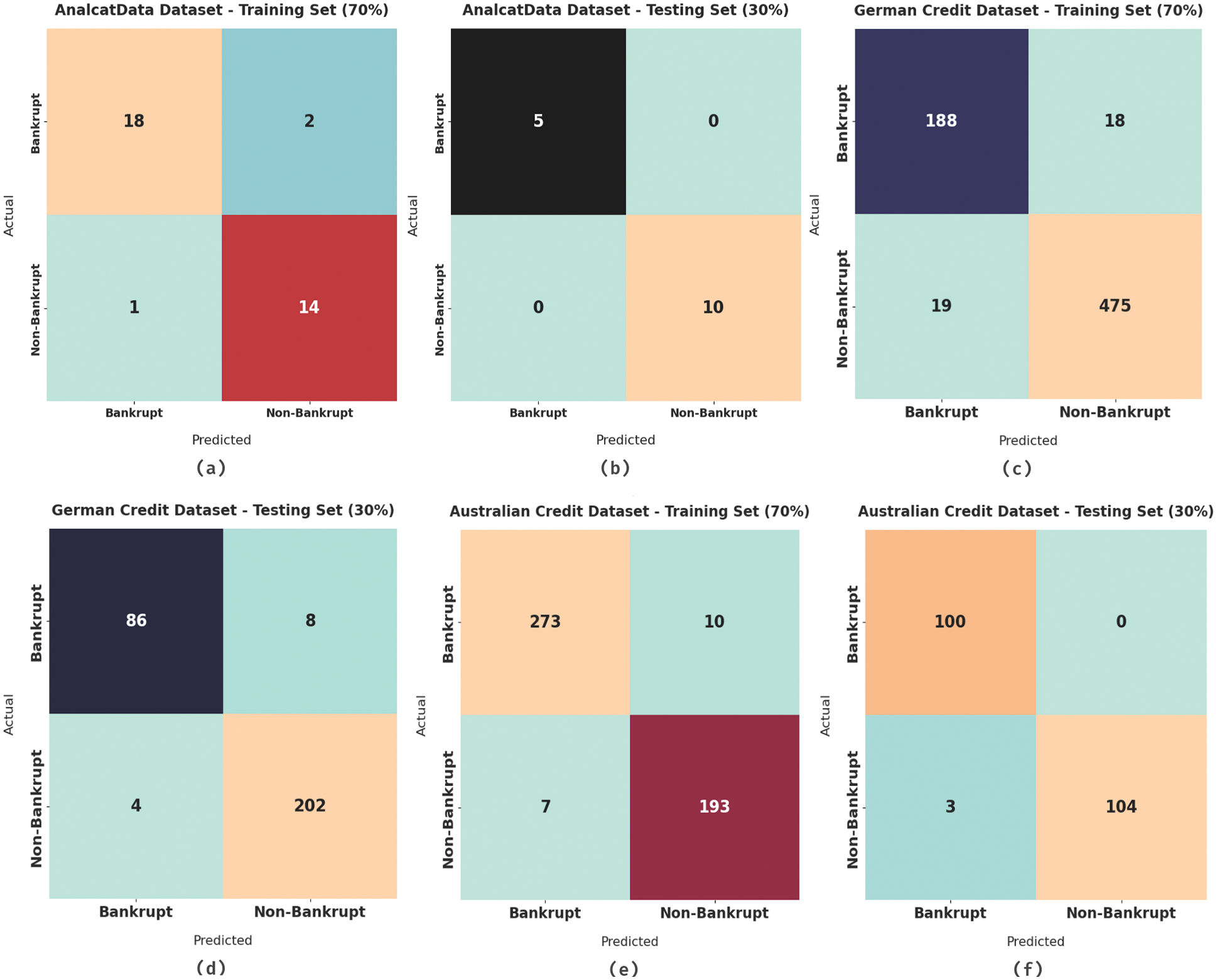
Figure 4: Confusion matrix of MVOFS-OVAE technique under different datasets

Tab. 4 demonstrates the overall FCP outcomes of the MVOFS-OVAE model on the test dataset in terms of different measures [24]. On 70% of training data on the Analcatdata dataset, the MVOFS-OVAE model has provided accuy , sensy , specy , Fscore , and MCC of 91.43%, 91.67%, 91.67%, 91.32%, and 82.78% respectively. Similarly, on 30% of testing data on the Analcatdata dataset, the MVOFS-OVAE model has attained accuy , sensy , specy , Fscore , and Mathew Correlation Coefficient (MCC) of 91.43%, 93.33%, 90%, 90.32%, and 82.78% respectively. Besides, on 70% of the German credit dataset training data, the MVOFS-OVAE model has provided accuy , sensy , specy , Fscore , and MCC of 94.71%, 93.71%, 93.71%, 93.65%, and 87.29% respectively. Similarly, on 30% of the German credit dataset testing data, the MVOFS-OVAE model has attained accuy , sensy , specy , Fscore , and MCC of 96%, 94.77%, 94.77%, 95.30%, and 90.64% respectively.

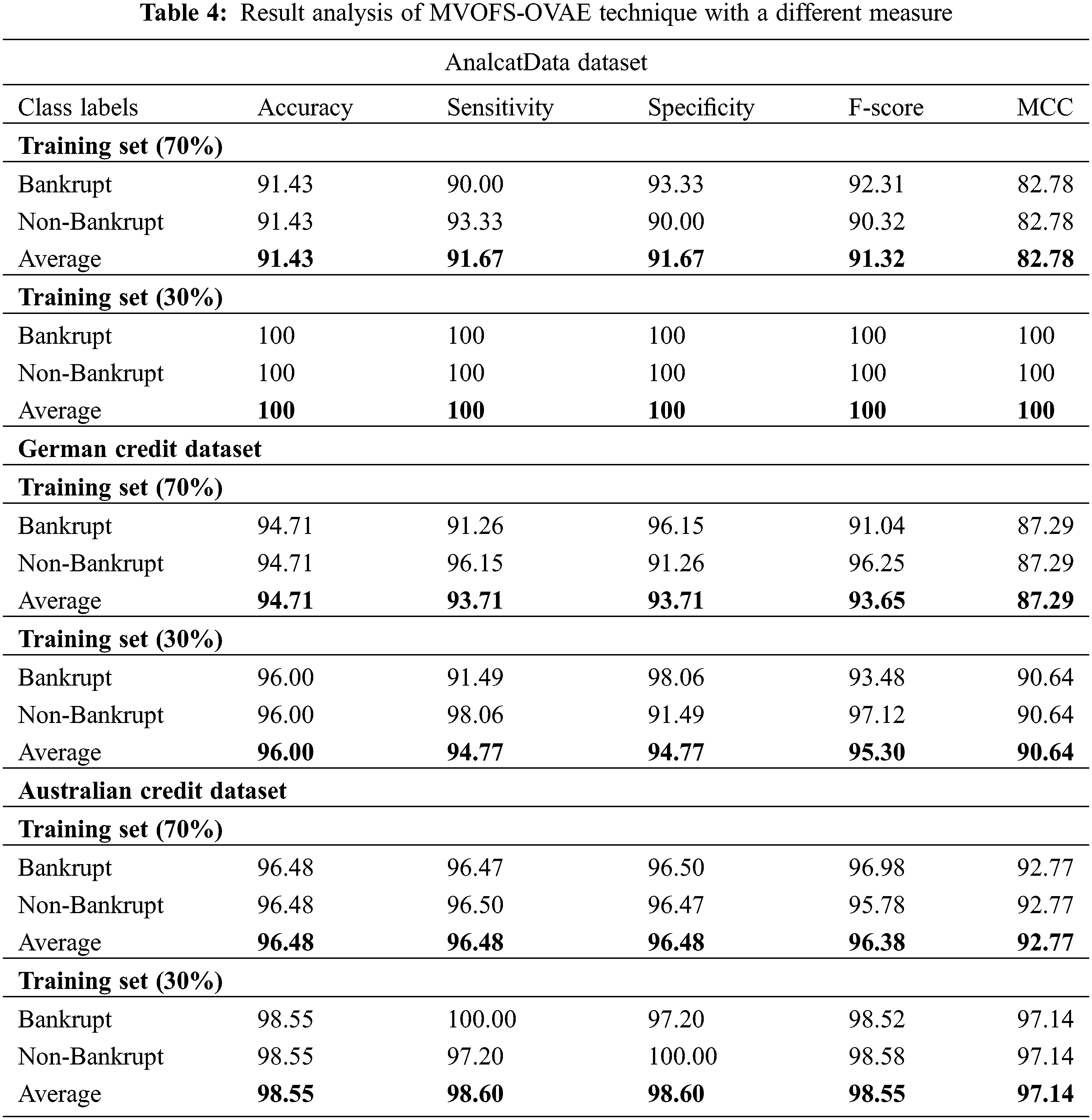
On 70% of training data on the Australian credit dataset, the MVOFS-OVAE model has provided accuy , sensy , specy , Fscore , and MCC of 96.48%, 96.48%, 96.48%, 96.38%, and 92.77% respectively. Similarly, on 30% of testing data on the Australian credit dataset, the MVOFS-OVAE model has attained accuy , sensy , specy , Fscore , and MCC of 98.55%, 98.60%, 98.60%, 98.55%, and 97.14% respectively.

Fig. 5 provides the accuracy and loss graph analysis of the MVOFS-OVAE technique on three datasets. The results show that the accuracy value tends to increase and the loss value tends to decrease with an increase in epoch count. It is also observed that the training loss is low and validation accuracy is high on three datasets.

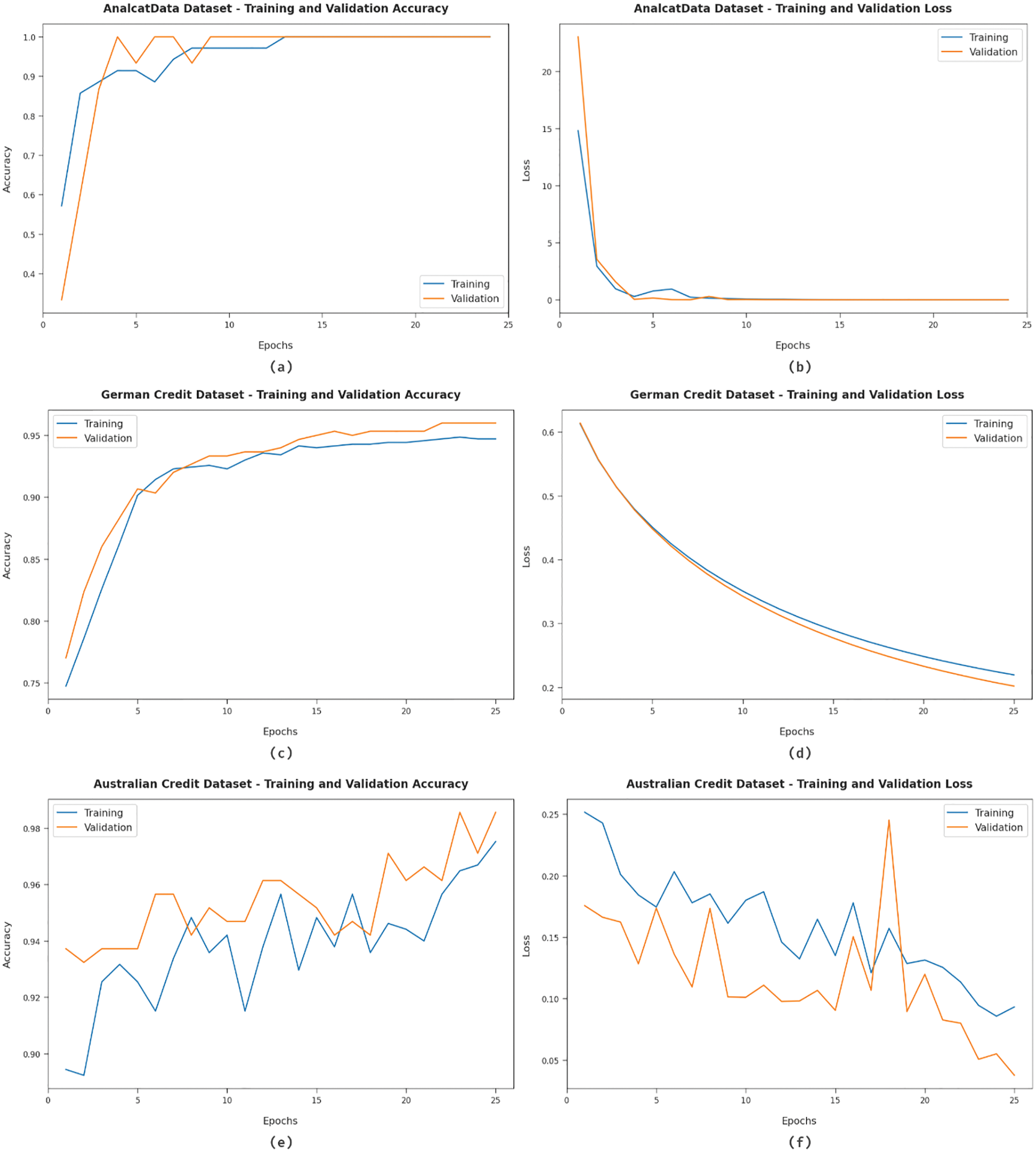
Figure 5: Accuracy and loss analysis of MVOFS-OVAE technique on three datasets

Fig. 6 exhibits a detailed comparative study of the MVOFS-OVAE approach on the AnalcatData dataset [25]. The figure reported that the AdaBoost method has shown the leastperformance over the other methods with sensy , specy , accuy , Fscore , and MCC of 65.98%, 68.04%, 66.38%, 66.81%, and 64.85% correspondingly. Next, the MLP and SVM methods have accomplished certainly improved results. In line with this, the QABOLSTM, LSTM-RNN, and ACO models have reached reasonable classification performance. However, the proposed MVOFS-OVAE model has gained maximum performance with sensy , specy , accuy , Fscore , and MCC of 100%, 100%, 100%, 100%, and 100% respectively.

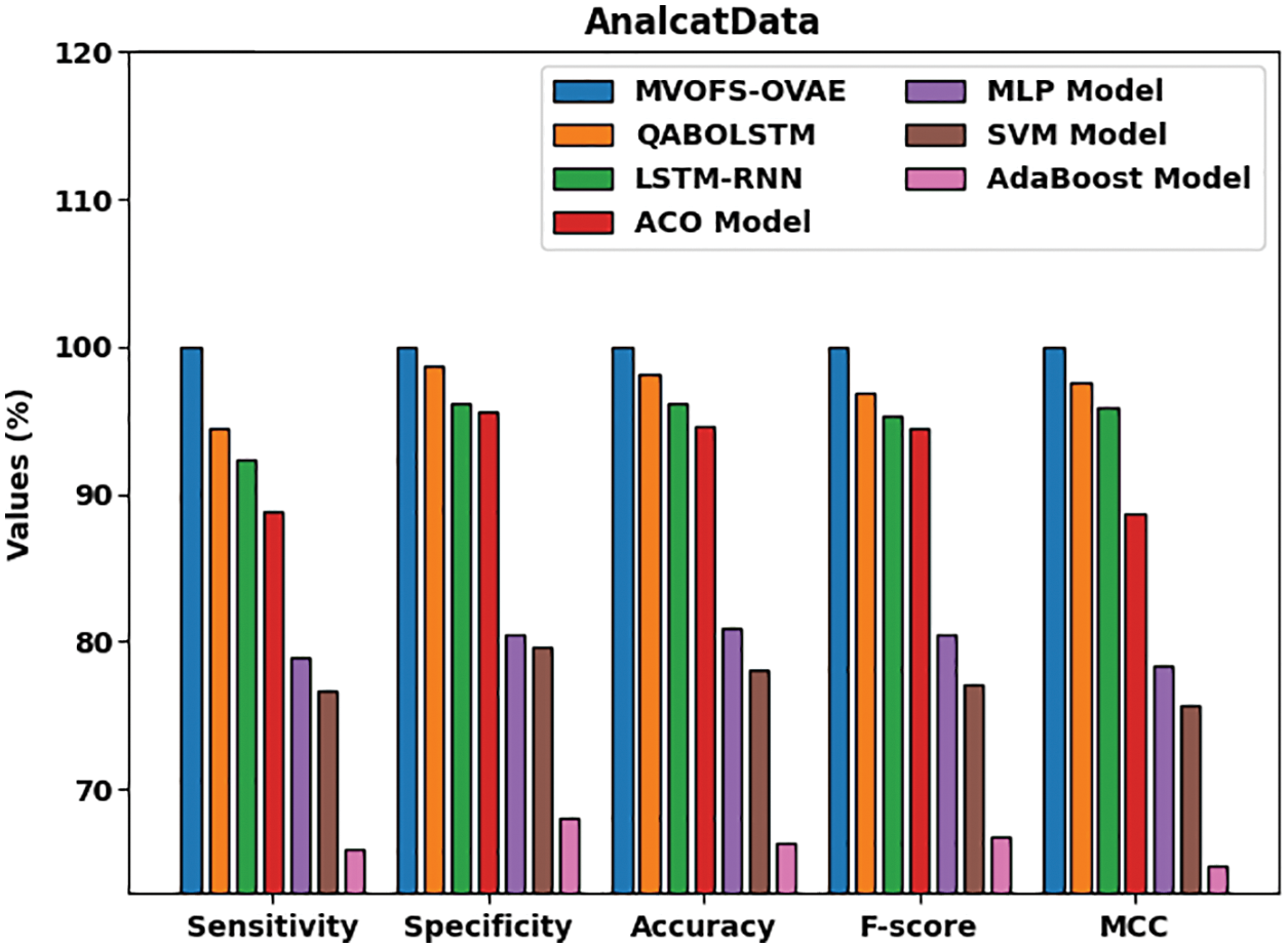
Figure 6: Comparative analysis of MVOFS-OVAE technique on AnalcatData dataset

Fig. 7 demonstrates a detailed comparative study of the MVOFS-OVAE model on the German credit dataset [25]. The figure reported that the AdaBoost approach has shown the least performance over the other methods with sensy , specy , accuy , Fscore , and MCC of 71.32%, 63.46%, 67.60%, 70.13%, and 40.13% correspondingly. Besides, the MLP and SVM approaches have accomplished certainly improved results. In line with this, the QABOLSTM, LSTM-RNN, and ACO models have reached reasonable classification performance. Lastly, the proposed MVOFS-OVAE model has gained maximum performance with sensy , specy , accuy , Fscore , and MCC of 94.77%, 94.77%, 96%, 95.30%, and 90.64% correspondingly.

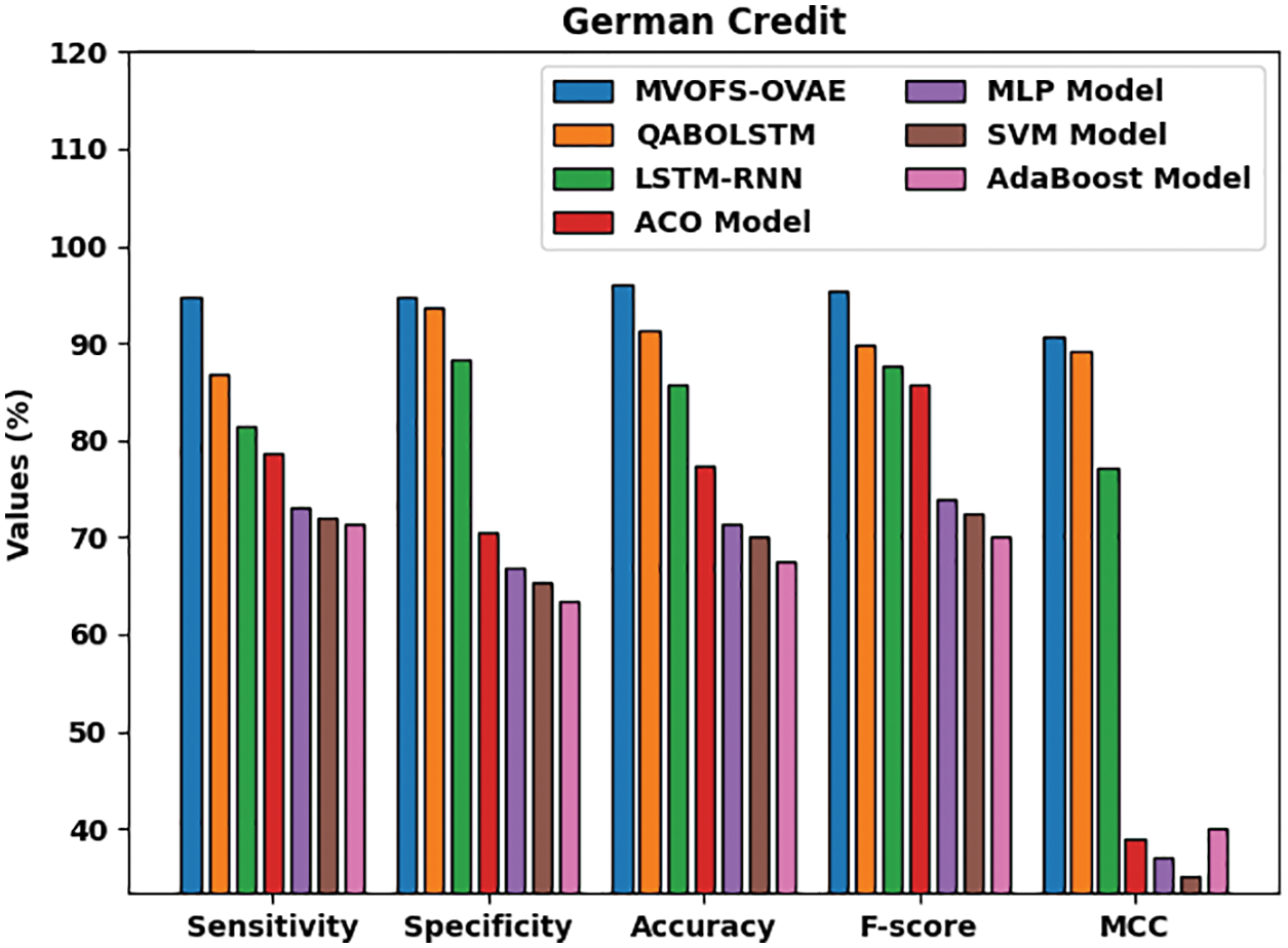
Figure 7: Comparative analysis of MVOFS-OVAE technique on German credit dataset

Fig. 8 exhibits a detailed comparative study of the MVOFS-OVAE technique on the Australian credit dataset. The figure reported that the AdaBoost method has shown the least performance over the other methods with sensy , specy , accuy , Fscore , and MCC of 71.32%, 69.33%, 69.46%, 68.07%, and 61.43% correspondingly. Then, the MLP and SVM approaches have accomplished certainly improved results. Also, the QABOLSTM, LSTM-RNN, and ACO models have reached reasonable classification performance. But, the proposed MVOFS-OVAE model has gained maximum performance with sensy , specy , accuy , Fscore , and MCC of 98.60%, 98.60%, 98.55%, 98.55%, and 97.14% respectively. Afterward examining the detailed results and discussion, the proposed MVOFS-OVAE model has ensured effective performance on all the test datasets. The enhanced performance of the proposed model is due to the optimal selection of features using the MVOFS technique and parameter optimization process.

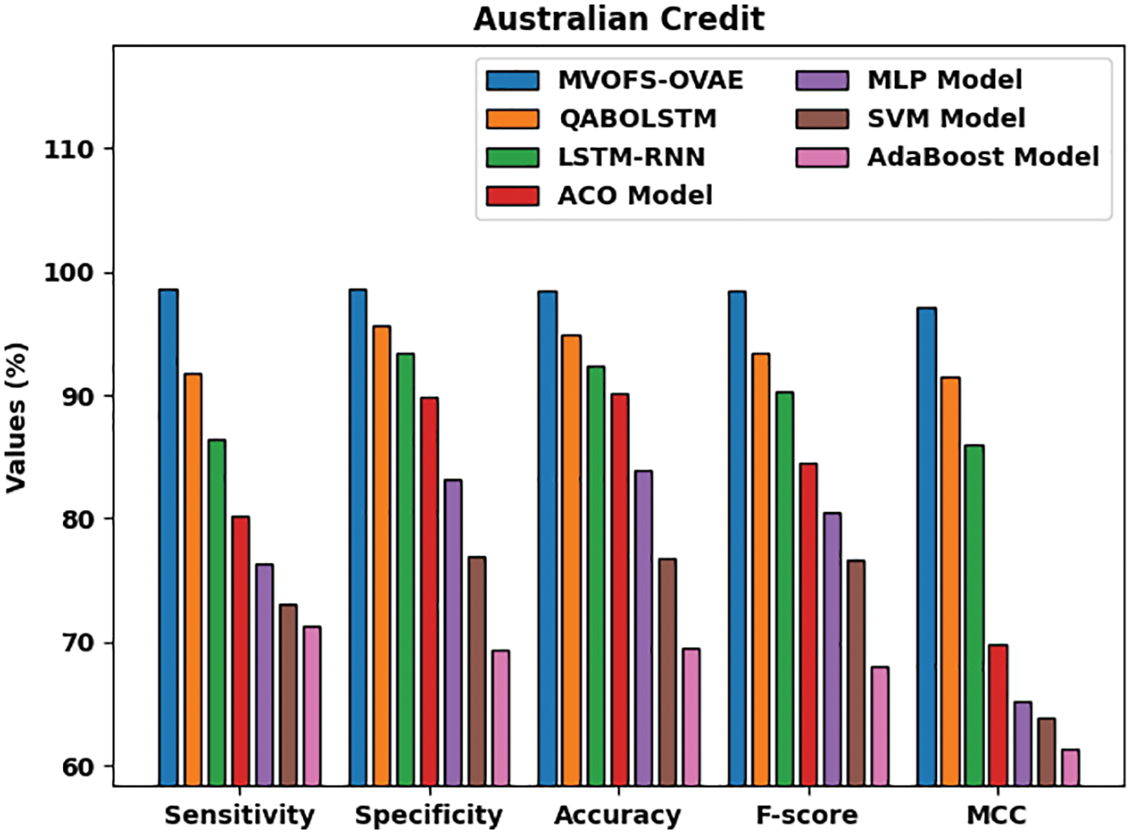
Figure 8: Comparative analysis of MVOFS-OVAE technique on Australian credit dataset

4  Conclusion

A new MVOFS-OVAE model has been developed in this research to foresee the financial crisis. The suggested MVOFS-OVAE model used min-max normalization to pre-process the input financial data. After that, the MVOFS approach is used to identify the best feature subsets. The VAE model is then used to divide financial data into two categories: financial crisis and non-financial crisis. Finally, the DE method is used to tune the parameters of the VAE model. The MVOFS-OVAE strategy outperformed the latest state-of-the-art approaches in a series of simulations on the benchmark dataset. As a result, the MVOFS-OVAE model can be used to forecast financial crises. The performance of the MVOFS-OVAE technique can be improved in the future by developing outlier reduction approaches.

Funding Statement: The authors received no specific funding for this study.

Conflicts of Interest: The authors declare that they have no conflicts of interest to report regarding the present study.

References

1. J. Uthayakumar, N. Metawa, K. Shankar and S. K. Lakshmanaprabu, “Intelligent hybrid model for financial crisis prediction using machine learning techniques,” Information Systems and e-Business Management, vol. 18, no. 4, pp. 617–645, 2020. [Google Scholar]
2. A. Samitas, E. Kampouris and D. Kenourgios, “Machine learning as an early warning system to predict financial crisis,” International Review of Financial Analysis, vol. 71, no. 2, pp. 101507, 2020. [Google Scholar]
3. P. K. Donepudi, M. H. Banu, W. Khan, T. K. Neogy, A. B. M. Asadullah et al., “Artificial intelligence and machine learning in treasury management: A systematic literature review,” International Journal of Management (IJM), vol. 11, no. 11, pp. 13–22, 2020. [Google Scholar]
4. H. Kim, H. Cho, D. Ryu and D, “Corporate default predictions using machine learning: Literature review,” Sustainability, vol. 2, no. 16, pp. 6325, 2020. [Google Scholar]
5. S. Kim, S. Ku, W. Chang and J. W. Song, “Predicting the direction of US stock prices using effective transfer entropy and machine learning techniques,” IEEE Access, vol. 8, pp. 111660–111682, 2020. [Google Scholar]
6. M. H. Fan, M. Y. Chen and E. C. Liao, “A deep learning approach for financial market prediction: Utilization of Google trends and keywords,” Granular Computing, vol. 6, no. 1, pp. 207–216, 2021. [Google Scholar]
7. J. Beutel, S. List and G. Von Schweinitz, “Does machine learning help us predict banking crises?,” Journal of Financial Stability, vol. 45, no. 3, pp. 100693, 2019. [Google Scholar]
8. A. Petropoulos, V. Siakoulis, E. Stavroulakis and N. E. Vlachogiannakis, “Predicting bank insolvencies using machine learning techniques,” International Journal of Forecasting, vol. 36, no. 3, pp. 1092–1113, 2020. [Google Scholar]
9. L. Alessi and R. Savona, Machine Learning for Financial Stability, Data Science for Economics and Finance. Cham: Springer, pp. 65–87, 2021. [Google Scholar]
10. M. Injadat, A. Moubayed, A. B. Nassif and A. Shami, “Machine learning towards intelligent systems: Applications, challenges, and opportunities,” Artificial Intelligence Review, vol. 54, no. 5, pp. 3299–3348, 2021. [Google Scholar]
11. G. Perboli and E. Arabnezhad, “A machine learning-based DSS for mid and long-term company crisis prediction,” Expert Systems with Applications, vol. 174, no. 4, pp. 114758, 2021. [Google Scholar]
12. N. Antulov-Fantulin, R. Lagravinese and G. Resce, “Predicting bankruptcy of local government: A machine learning approach,” Journal of Economic Behavior & Organization, vol. 183, no. 2, pp. 681–699, 2021. [Google Scholar]
13. T. Wang, S. Zhao, G. Zhu and H. Zheng, “A machine learning-based early warning system for systemic banking crises,” Applied Economics, vol. 53, no. 26, pp. 2974–2992, 2021. [Google Scholar]
14. L. Machado and D. Holmer, “Credit risk modelling and prediction: Logistic regression versus machine learning boosting algorithms,” Ph.D. dissertation. Uppsala Universitet, Sweeden, 2022. [Google Scholar]
15. N. Metawa, I. V. Pustokhina, D. A. Pustokhin, K. Shankar and M. Elhoseny, “Computational intelligence-based financial crisis prediction model using feature subset selection with optimal deep belief network,” Big Data, vol. 9, no. 2, pp. 100–115, 2021. [Google Scholar]
16. S. Sankhwar, D. Gupta, K. C. Ramya, S. Sheeba Rani, K. Shankar et al., “Improved grey wolf optimization-based feature subset selection with fuzzy neural classifier for financial crisis prediction,” Soft Computing, vol. 24, no. 1, pp. 101–110, 2020. [Google Scholar]
17. X. Ma and S. Lv, “Financial credit risk prediction in internet finance driven by machine learning,” Neural Computing and Applications, vol. 31, no. 12, pp. 8359–8367, 2019. [Google Scholar]
18. D. Liang, C. C. Lu, C. F. Tsai and G. A. Shih, “Financial ratios and corporate governance indicators in bankruptcy prediction: A comprehensive study,” European Journal of Operational Research, vol. 252, no. 2, pp. 561–572, 2016. [Google Scholar]
19. J. Uthayakumar, N. Metawa, K. Shankar and S. K. Lakshmanaprabu, “Financial crisis prediction model using ant colony optimization,” International Journal of Information Management, vol. 50, no. 5, pp. 538–556, 2020. [Google Scholar]
20. S. Mirjalili, S. M. Mirjalili and A. Hatamlou, “Multi-verse optimizer: A nature-inspired algorithm for global optimization,” Neural Computing and Applications, vol. 27, no. 2, pp. 495–513, 2016. [Google Scholar]
21. D. P. Kingma and M. Welling, “Auto-encoding variational bayes,” arXiv. arXiv:1312.6114, 2013. [Google Scholar]
22. Y. Yang, K. Zheng, C. Wu and Y. Yang, “Improving the classification effectiveness of intrusion detection by using improved conditional variational autoencoder and deep neural network,” Sensors, vol. 19, no. 11, pp. 2528, 2019. [Google Scholar]
23. W. Deng, J. Xu, Y. Song and H. Zhao, “Differential evolution algorithm with wavelet basis function and optimal mutation strategy for complex optimization problem,” Applied Soft Computing, vol. 100, no. 15, pp. 106724, 2021. [Google Scholar]
24. J. Uthayakumar, T. Vengattaraman and P. Dhavachelvan, “Swarm intelligence based classification rule induction (CRI) framework for qualitative and quantitative approach: An application of bankruptcy prediction and credit risk analysis,” Journal of King Saud University-Computer and Information Sciences, vol. 32, no. 6, pp. 647–657, 2020. [Google Scholar]
25. S. K. S. Tyagi and Q. Boyang, “An intelligent internet of things aided financial crisis prediction model in FinTech,” IEEE Internet of Things Journal, pp. 1, 2021. DOI https://doi.org/10.1109/JIOT.2021.3088753. [Google Scholar]
Cite This Article
Copyright © 2023 The Author(s). Published by Tech Science Press.
This work is licensed under a Creative Commons Attribution 4.0 International License , which permits unrestricted use, distribution, and reproduction in any medium, provided the original work is properly cited.
Downloads
Citation Tools