Detection of Diabetic Retinopathy from Retinal Images Using DenseNet Models

1  Introduction

One of the most prevalent diseases around the world is Diabetic Mellitus. The extended prevalence of diabetes causes several problems related to health, such as Diabetic Retinopathy, nephropathy, diabetic foot, etc. The most common issue is Diabetic Retinopathy (DR). Diabetic Retinopathy is a diabetes complication that can harm the retina’s veins and leads to significant vision loss. Diabetic Retinopathy typically happens when high glucose levels damage the veins and limit the bloodstream to the retina. Initially, it starts with no symptoms or mild vision problems, and eventually, it can create vision loss. The symptoms can be noticed only when it reaches an advanced stage and usually affects both eyes [1]. Therefore, this disease must be treated at an early stage and can help to prevent vision loss. Still, since it takes time for diagnosis and there is a shortage of ophthalmologists, patients suffer vision loss even before diagnosis. Hence, early detection of DR may help in reducing the problem. However, many physical tests are required to detect DR, like visual acuity, pupil dilation, tonometry, etc. And also, it is challenging to identify through the tests during the earlier stage of the disease [2]. Therefore, a new diagnostic technique must identify the disease before it is visible on the exam to treat in the earlier stage itself. Therefore, there is a severe need for some good Computer-Aided Diagnosis (CAD) to accelerate this process.

Even though there are many computer-aided diagnosis tools, detecting diabetic retinopathy at some severity level is challenging, such as mild and moderate DR. The principal target of the work is to apply the data fusion/feature fusion technique, which combines more than one relevant feature to predict diabetic retinopathy at an early stage with greater accuracy. It usually takes about 7–14 days in conventional methods to detect DR, considering the eye screening and consulting from an ophthalmologist. Since we are using an end-user neural network to detect and classify, it takes around 2–5 min depending on the resolution of the fundus image since there aren’t any methods as of yet which is practically attainable to click the fundus images sitting at home so the person might first take a pre-screening or undergo usual fundoscopy after which the patient may use the neural network to detect DR [3].

There are two types of Diabetic Retinopathy: Non-Proliferative DR (L0, L1, L2, L3) & Proliferative (L4) DR. Microaneurysms, cotton wool spots, and hemorrhages define non-proliferative retinopathy; and iris or retinal neovascularization defines proliferative retinopathy. Non-Proliferative DR (NPDR) is the milder form. It is primarily symptomless, whereas Proliferative DR (PDR) is an advanced stage of DR, and it leads to the formation of abnormal blood vessels in the retina [4]. It causes severe loss during this stage. These features are examined by ophthalmoscopy or fundus images, and they can be graded in clinical terms as Normal, having no abnormalities; Mild, where only microaneurysms are present; Moderate containing multiple microaneurysms along with dot and blot hemorrhages and cotton wool spots in one quadrant; Severe, defined by the presence of microaneurysms and severe hemorrhages in all four quadrants along with wool spots present in at least two quadrants and intraretinal microvascular abnormalities present in more than one quadrant, and lastly, Very Severe/Proliferative, where neovascularization or vitreous/preretinal hemorrhage occurs [5]. This final grade is the stage of DR where treatment is challenging. The proposed work consists of three models where pretrained densnet121 and desnsenet169 have been used and altered according to the needs of the problem to be tackled.

The paper proceeds in the following way: Related work about Diabetic Retinopathy is reviewed in Section 2. The proposed implementation model includes the data overview and steps like ben graham preprocessing, scaling and cropping, etc. A detailed description of the three proposed dense Convolutional Neural Networks (CNN) models is described in Section 3. The visual performance evaluation and comparison of the models on the Kaggle 2015 dataset are shown in Section 4. In the end, in Section 5, the conclusions and future scope are presented.

2  Related Works

Pires et al. (2019) [2] introduced a method for data analysis and interpretation to bring out an efficient software process model directly from the retina images to provide a DR detector by using CNN. They found that, with a set of specific instructions, the performance of CNN can be enhanced to a certain level. Also, it was possible to implement high goal networks by using several low goal networks in the introductory phase: higher resolution images, improper image quality, and hardware-specific issues. Dataset utilized was Kaggle fundus. The information-driven technique portrayed here beats all past solutions with an AUC of 98.0%. Though the better results were obtained the understanding about the model how it reaches the decision was challenging by the method introduced.

Sarwinda et al. (2018) [6] proposed the model categorizing different stages of diabetic retinopathy mainly into three subclasses: normal, mild non-proliferative diabetic retinopathy and moderate or severe non-proliferative diabetic retinopathy. They used Histogram of Gradient for texture feature extraction, factor analysis for feature selection, random forest and support vector machines technique for shallow learning, and high-performance evaluation. Drawbacks were gentle: NPDR vs. Ordinary has a lower exactness than other parallel classifications. Dataset utilized was the DiaretDB0 public database. The proposed strategy accomplished around 85% precision for the double class arrangement.

In Khojasteh et al. (2018) [7], the study embedded a pre-processing layer before the first convolutional neural network layer and a new convolutional neural network framework with eleven layers resulting in a modified version of the convolutional neural network. They used two image enhancement techniques: contrast enhancement and to operate on smaller regions of the image contrast limited adaptive histogram equalization, separately, in the pre-processing layer for improved accuracy in the identification of exudates, hemorrhages and microaneurysms. This structure improved the absolute precision of 87.6% and 83.9% for the difference upgrade and differentiation restricted versatile histogram adjustment layers separately. Further, the accuracy of the convolutional neural framework alone, excluding the pre-processing layer, was 81.4%. The accuracy of the model is comparatively low and only binary classification of the DR disease detection is performed.

This proposed work by Costa et al. (2018) [8] performed their study to find an alternative to avoid the need for retinal lesions annotated manually, at pixel level by a specialist as training data. They established a new method centered on multiple instances learning and bag of visual words by utilizing the implicit findings present on annotations made at pathological images and achieved better mid-level representations of the images through the joint optimization of the instance encoding and the image classification stages. In addition, a new loss function is introduced to constrain the mid-level representations of pathological images to enhance their interpretability. The model interpretability was enhanced and mainly binary classification is performed. Different levels of DR severity was not calculated by the model.

Dutta et al. (2018) [9] realized the necessity of processing the fundus images to extract key features and carried out their study using classical neural networks (BNN), deep neural networks (DNN) and convolutional neural networks (CNN) for the training of the model. They succeeded in quantifying each feature element into different classes through fuzzy c-means and removing noise using the median filter technique. Dataset utilized was Messidor. Accuracy for BNN in training was 62.7% in testing was 42%, for CNN in training was 76.4% in testing was 78.3%, for DNN in training was 89.6%, and for testing was 86.3%. The number of retinal images used for training and testing was less, and accuracy could have been better.

Kumar et al. (2018) [10] established a methodology for green channel extraction and histogram equalization. After the pre-processing, the images were equally illuminated, image intensities were adjusted, and contrast was enhanced and used other morphological procedures too for the same. Linear Support vector machine was used to categorize the DR, which helped develop a new method for detecting diabetic retinopathy by precisely determining the quantity and location of microaneurysms. This proposed technique had a sensitivity of 96% and a specificity of 92% for DR detection. The disadvantage of this approach is that it only considers microaneurysms and excludes other characteristics such as cotton wool spots, exudates, and aberrant blood vessels.

Generally, in contrasting the exhibition and examining the aftereffects of conventional and Deep Learning-based techniques, the DL-based strategies beat the traditional methods, as discussed in the writing study. On separately auditing the DL-based procedures, Conventional Neural networks (CNN) and their pre-prepared structures have been utilized by the more significant part of the specialists. It has delivered more possible outcomes. Be that as it may, CNN experiences various issues; one of them is information comment, where it requires the ophthalmologists’ administrations to name the retinal fundus pictures. Class irregularity and overfitting are different issues that may bring about one-sided expectations. An expansion in information builds the exhibition of the based frameworks, which may not be conceivable in a wide range of issues. Robotized DR Disease recognition frameworks astoundingly decrease the determination time cost and help ophthalmologists identify retinal variations from the norm and give timely treatment. A few examinations have proposed that the exhibition has been expanded while incorporating the handmade and CNN-based highlights.

Later on, CNN designs can be coordinated to remove more exact and better picture highlights, which improve DR recognition and grouping rate. At first, in this work, a concise depiction was given on clinical picture preparation, Diabetic Retinopathy hazard elements, and characterizations. Regular and DL-based DR discovery techniques are examined, alongside their exhibition measurements. The majority of the specialists have utilized CNN for its proficiency and capacity to give more exact outcomes, which outperforms different strategies. This survey paper examines the ongoing works, and the most valuable methods are advanced, which helps the exploration network recognize and order DR.

3  Implementation

In the proposed work, Fundus images of patients’ eyes affected by DR are used to train high-density CNN’s, i.e., DenseNets, which can classify images into five classes (mild DR without DR, medium DR, severe, proliferative DR). The first and foremost important step is image preprocessing and separation into grayscale. The model goes through various stages. First, image preprocessing ensures that impurities such as starting noise and uneven contrast lighting are not included in the image. Then, after reducing the impact of light, cropping areas with less information, classify and predict using a dense convolutional neural network model.

3.1 Image Preprocessing

The image contains many removal conditions, including blurred vision, negative or unsatisfactory color vision drift, and partial vision that can confuse the result. However, the proposed method worked with these noisy data to increase sensitivity and accuracy to overcome these efforts. In the entire process, the input image data is first converted to a grayscale image, reducing the influence of light conditions. Since the input image size in the DR dataset is considered to be very high resolution, the training process is slowed down, and there is a possibility that the training process consumes and runs out of memory. For this purpose, the image is scaled to a resolution of 224 × 224. In addition, areas without image information have been truncated. Finally, Ben Graham’s pre-processing method for improving lighting conditions. Algorithm 1 below states the same. The normal retinal image and the image after performing Ben Graham’s pre-processing are shown in Figs. 1a and 1b.

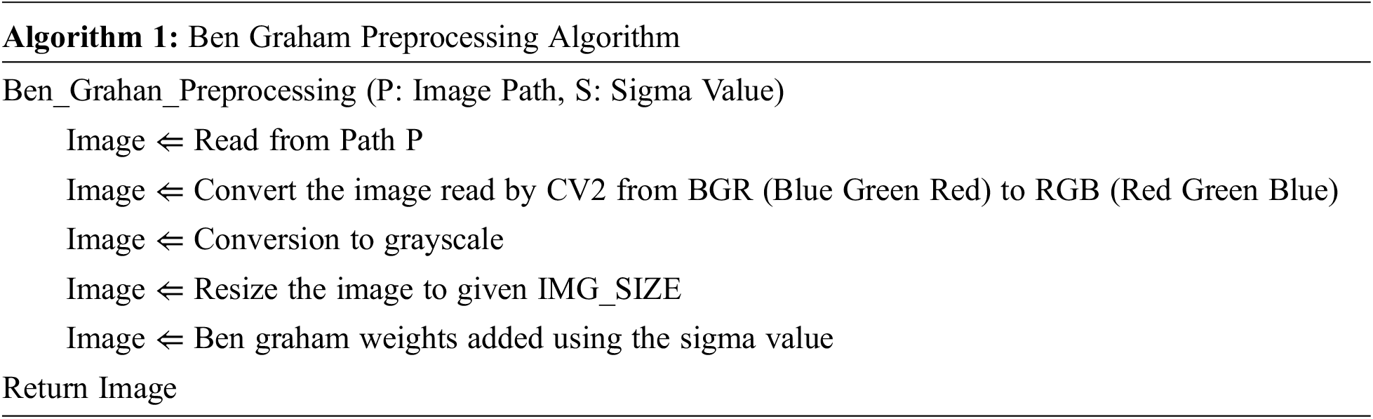
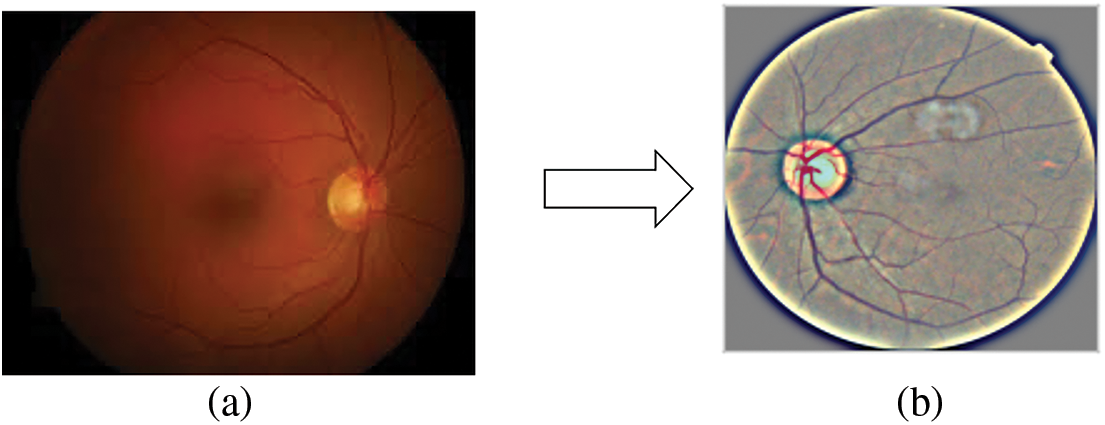
Figure 1: (a) Real Retinal Image (b) Ben Graham pre-processing

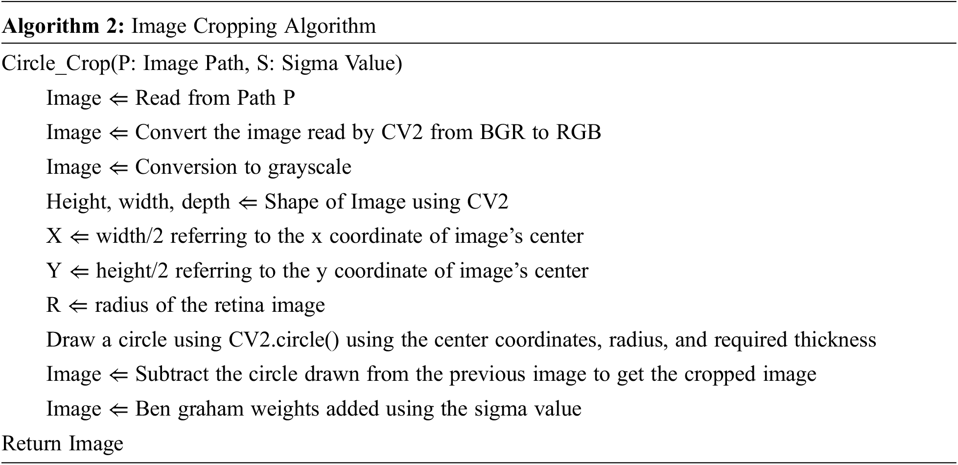
Furthermore, uninformative black areas of the images have been cropped. Algorithm 2 below states the same.

Figs. 2a, 2b, and 2c shows the normal retinal image, Ben Graham’s pre-processing image and the cropped image. Since the training data set has about 3600 images which are comparatively lesser on an excellent model formation, data creation and mixture are introduced to lead random transformations into our datasets (vertically/dimensionally horizontal, rotate, rotate, zoom). This helps our model that making the pictures more generalized. Then many labels were created, which makes it a multi-label problem for the prediction. Instead of predicting a single label, we change your goals in multi-route questions. If the goal is a specific level, it represents all classes before. Now the images can be provided in the proposed CNN models.

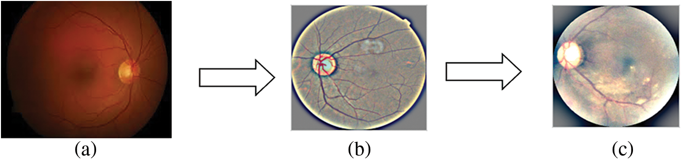
Figure 2: (a) Real Retinal Image, (b) Ben Graham pre-processing, (c) Pre-processing followed by cropping

3.2 Proposed CNN Model

The project has a variety of pre-trained models and proposes three different high-density CNN models for adding new layers experimented with. Choosing the suitable design parameters for your CNN directly impacts your model’s performance. Densely Connected Convolutional Networks were chosen for this model because DenseNets has several decisive advantages. It alleviates burnishing gradients, enhances functional propagation, encourages practical reuse, and significantly reduces parameters.

DenseNets require fewer parameters than a typical CNN, because there are no redundant feature maps to learn. Also, DenseNets concatenate the layer’s output feature maps with the input feature maps instead of adding them together. A network contains N layers each of which executes a non-linear transformation TN.

The dense connectivity in the DenseNet architecture is represented using Eq. (1).

TN=TN+([Q0Q1,…..QN−1]) (1)

where [ Q0Q1,…..QN−1 ] is the concatenation of the feature maps generated by the [0, 1, …. Nth] layers. QN represent the output of the Nth layer of the network and Q0 represent the input image.

DenseNets are partitioned into DenseBlocks, where the feature map dimensions remain constant inside a block but the number of filters varies. Since the feature maps are concatenated, the channel dimension grows with each layer. It can be generalized for the Nth layer if we make TN to produce R feature maps every time.

RN=R0+R∗(N−1) (2)

where R is the growth rate. Because of its dense connectedness, this network architecture is referred to as a Dense Convolutional Network [11].

The first model is based on the DenseNet-121 model. These networks begin with a simple convolution and pool hierarchy. There is a dense block, then a layer of transition, then another dense block and another layer of transition, another dense block and a layer of transition, and finally a dense block following a layer of classification. The starting block of convolution is 7 × 7 in size, has two strides, and has 64 filters. Then, following it is a 3 × 3 Max Pooling layer with stride 2. Then there is the dense block. All dense blocks have two convolutions along with 1 × 1 and 3 × 3 size kernels. Dense block one can be repeated six times in a row, dense block twelve times for a couple, dense block three twenty-four times, and finally dense block four sixteen times. Every dense layer is a layer of transition consisting of a 1 × 1 convolution layer and an average pool of 2 × 2 layers with a stride length of 2. After the last dense layer of the model is the world average pool layer. Regularization is done using the 0.5 dropouts. After the fully connected layer, the softmax function continues to convert the output into a probability distribution. The architecture of model1 is shown in Fig. 3.

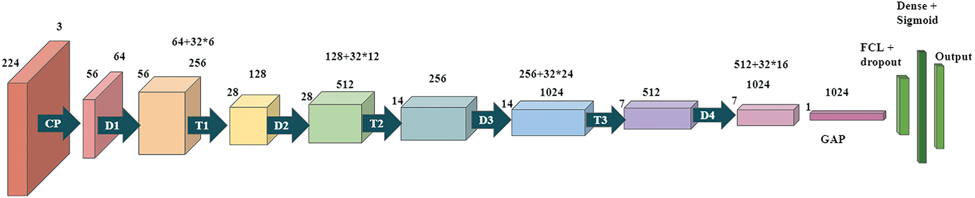
Figure 3: Proposed Dense CNN Model 1 based on DenseNet-121

The second model is based on the DenseNet-169 model. These networks begin with a simple convolution and pool hierarchy. There is a dense block, then a layer of transition, then another dense block and another layer of transition, another dense block and a layer of transition, and finally a dense block following a layer of classification. The starting block of convolution has a stride of 2 with 64 filters at size 7 × 7, followed by a max-pooling layer of 3 × 3 and a stride of 2. Next a dense block. All dense blocks have two convolutions with kernels of size 1 × 1 and 3 × 3. Dense block 1 to be repeated six times, dense block 2 to be repeated twelve times, dense block three to be repeated thirty-two times, and finally, dense block four may be repeated thirty-two times. Each dense layer is a transition layer with a 1 × 1 convolutional layer and an average pooled 2 × 2 layer of stride length 2. There is a global average pooling layer behind the last dense block in the model. Regularization is done using 0.5 dropouts. After the fully connected layer, the softmax function continues to convert the output into a probability distribution. The model2 architecture is demonstrated in Fig. 4.

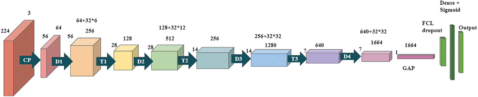
Figure 4: Proposed Dense CNN model 2 based on DenseNet-169

The third model is based on the DenseNet-121 model. These networks begin with a simple convolution and pool hierarchy. Followed by, there are dense blocks and the transition layers. The starting block of convolution is 7 × 7 in size, has two strides, and has 64 filters. Then, following it is a 3 × 3 Max Pooling layer with stride 2. Then there is the dense block. All dense blocks have two convolutions along with 1 × 1 and 3 × 3 size kernels. Dense block one can be repeated six times in a row, dense block twelve times for a couple, dense block three twenty-four times, and finally dense block four sixteen times. Every dense layer is a layer of transition consisting of a 1 × 1 convolution layer and an average pool of 2 × 2 layers with a stride length of 2. After the last dense layer of the model is the world average pool layer. Regularization is done by using a 0.5 of dropout. After the fully connected layer, the softmax function continues to convert the output into a probability distribution. Fig. 5 demonstrates the models with modified filter size and hyperparameter tuning.

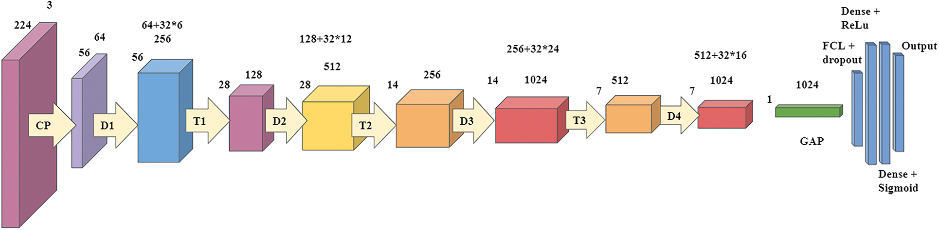
Figure 5: Proposed Dense CNN model 2 based on DenseNet-121

4  Results and Discussions

The model was executed on Google Colab and python version 3.7. It also required TensorFlow version 2.0 and Keras version 2.3.

4.1 Datasets Used

The Diabetic Retinopathy Dataset has been used for the data of color fundus images, which is provided by APTOS, which has an extensive collection of retinal images taken with the help of fundus photography under a wide range of lighting and imaging constraints. The data set contains 3,662 training images and 1928 testing images under variety of imaging conditions in which only training dataset has been in the proposed model. Each image has been assessed on a scale of 0 to 4 by a clinician for the severity of diabetic retinopathy. The data found related to this topic is noisy and requires multiple pre-processing steps to get all images to a usable format for training a model. The training dataset is the APTOS 2019 dataset [12], whereas the test dataset is the Kaggle 2015 dataset [13] from where well-shuffled 550 images have been chosen to test the best-proposed model. Kaggle 2015 dataset contains a total of 35,126 retina scan images to detect diabetic retinopathy. These images have been scaled to 224 × 224 pixels so that they can be utilized with a wide range of deep learning models that have already been trained.

4.2 Evaluation Metrics

The test dataset’s results are assessed using four factors: accuracy, precision, recall, and f1-score, all of which may be evaluated using the confusion matrix. TP, TN, FP, FN are true positive, true negative, false positive and false negative, respectively. Binary cross-entropy has been used, a particular type of cross-entropy with a goal of 0 or 1. The calculation is done with the formula of cross-entropy, where the target is converted to a one-hot vector like [0,1] or [1,0] and the predictions, respectively.

4.3 Training Performance Evaluation

This paper proposes three models of Dense CNN to classify DR into 1 out of 5 Diabetic Retinopathy classes according to the severity of the disease: No DR, Mild DR, Moderate DR, Severe DR, and proliferative DR. The images are trained on DenseNet based sequential models with the learning rate of 0.00005. It was also observed that significant changes in validation accuracy occurred only after epoch size 30 and above in all models. Therefore, epoch size and accuracy are not linearly related to each other. The larger the Epoch size, the better the performance. It was also found that Model 3 achieved the highest accuracy overall. In Model 3, maximum training accuracy of 93.51% was observed. Followed by it, Model 2 has reached 89.19% of training accuracy, and Model 1 has achieved the least of the three, i.e., 83.9% of training accuracy. After comparing the three models discussed above, Model 3 has achieved the highest accuracy; after that, Model 2 and then Model 1. The least accuracy is achieved by Model 1. The rate of accuracy is related to the proposed system and the parameters set for each model. Model 3 reduces the problem of overfitting to a great extent [14].

4.4 Training and Validation Results of Model 1, Model 2, and Model 3

The graph in Fig. 6a shows the comparison of the training accuracy and validation accuracy. The training goes through 50 epochs, as shown in the graph. A batch size of 32 has been maintained for the training of each epoch. The training accuracy obtained is 0.8390, while the validation accuracy obtained is comparatively less, around 0.8109. Thus, the training and validation accuracy range is pretty high. The model has achieved high evaluation metrics due to increased training and validation accuracy. The graph in Fig. 6b shows a comparison between the training loss and validation loss. The training goes through 50 epochs, as shown in the graph. The training loss achieved is 0.0183, while the validation loss obtained is 0.1399. The loss achieved on both training and validation is comparatively good. The increasing loss with epochs means increasing overfitting.

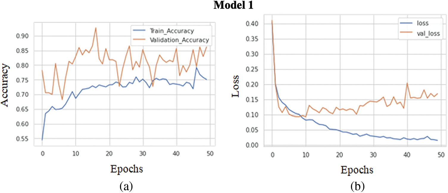
Figure 6: (a) Training accuracy V/S validation accuracy of model 1, (b) Training loss V/S validation loss of model 1

The graph in Fig. 7a shows the comparison of the training accuracy and validation accuracy. The training goes through 50 epochs, as shown in the graph. Same as before batch size of 32 has been maintained for the training of each epoch. The training accuracy obtained is 0.8919, while the validation accuracy obtained is comparatively less, around 0.8673. Training and validation accuracy range is pretty high. The model has achieved high evaluation metrics due to increased training and validation accuracy. The graph in Fig. 7b demonstrates a comparison between the validation loss and training loss. The training goes through 50 epochs, as shown in the graph. The training loss obtained is 0.0086, while the validation loss obtained is 0.0986. The loss received on both training and validation is comparatively good. The increasing loss with epochs means increasing overfitting.

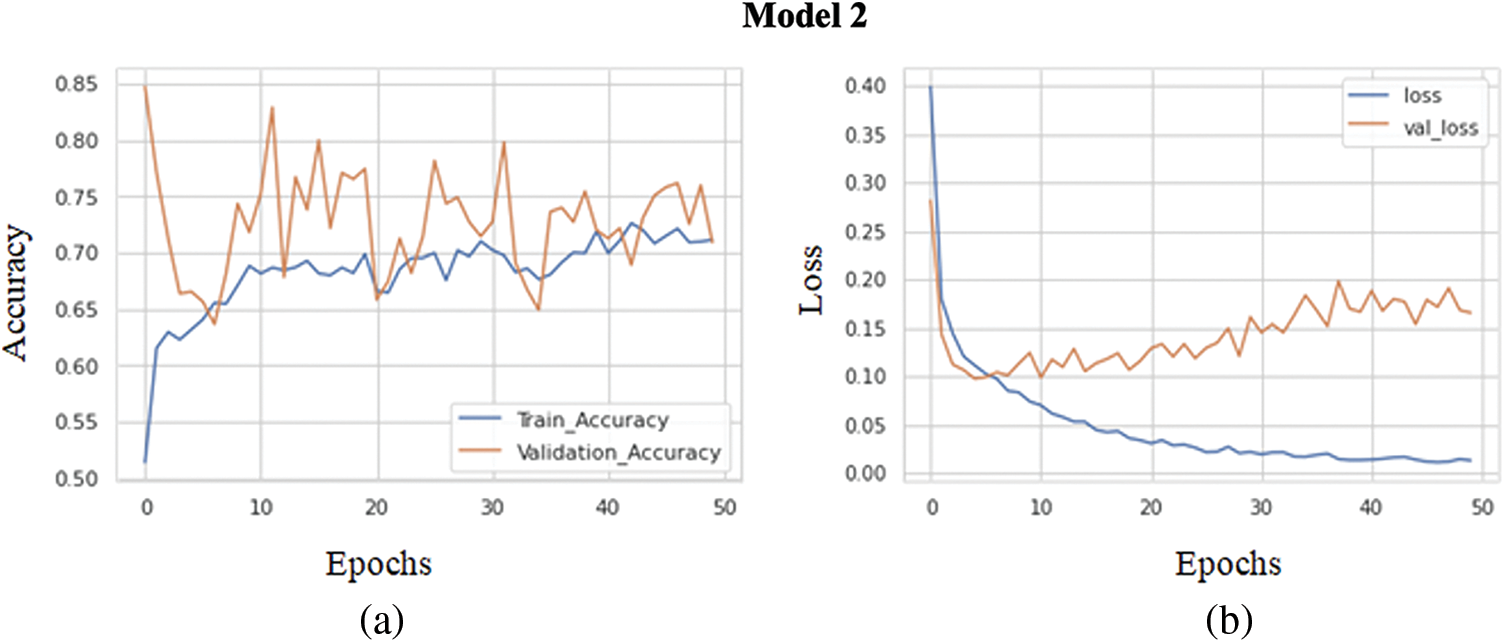
Figure 7: (a) Training accuracy V/S validation accuracy of model 2, (b) Training loss V/S Validation loss of model 2

A comparison between the training accuracy and validation accuracy is shown in Fig. 8a. The training goes through 50 epochs, as shown in the graph. Same as the previous model, a batch size of 32 has been maintained for the training of each epoch. The training accuracy obtained is 0.9351, while the validation accuracy obtained is comparatively less, around 0.9061. Thus, the training and validation accuracy range are relatively high. The model has achieved high evaluation metrics due to high training and validation accuracy. The graph in Fig. 8b compares between the validation loss and training loss. The training goes through 50 epochs, as shown in the graph. The training loss obtained is 0.0261, while the validation loss achieved is 0.0870. Thus, the loss received on both training and validation is comparatively good. This model reduces the increasing loss with increasing epochs in the previous models, i.e., overfitting is significantly reduced.

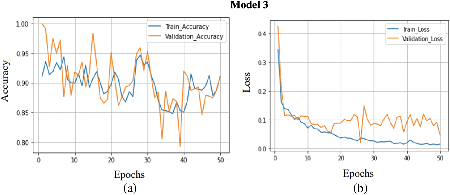
Figure 8: (a) Training accuracy V/S validation accuracy of model 3, (b) Training loss V/S Validation loss of model 3

4.5 Comparison Between the Models

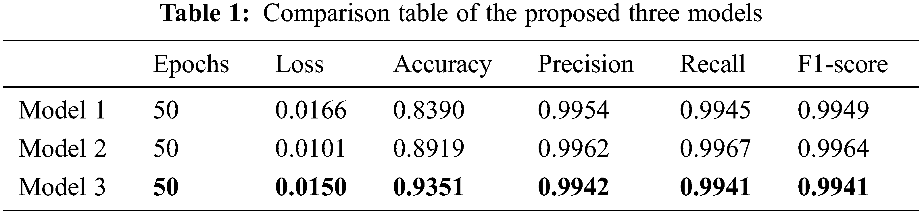
In this section, a comparison between the models is made. The three models have been compared based on five parameters. These three models have been trained over 3,662 images altogether and also for 50 epochs for uniformity. As a result, model 3 reduces overfitting greatly compared to model 1 and model 2.

Tab. 1 shows the comparison table of the proposed three models. Models 1, model 2, and model 3 obtained the highest accuracy of 0.83, 0.89, and 0.93 and precision of 0.9954, 0.9962, and 0.9942, respectively. Out of all the evaluation metrics calculated, model 3 outperformed the other two models 1 and 2 in terms of accuracy, model 1 outscored in precision and model 2 outperformed in recall and F1-score.

4.6 Testing Results Over Kaggle 2015 Dataset

Well-shuffled 550 images of the Kaggle Diabetic Retinopathy dataset (2015) have been pre-processed with the methods mentioned above and taken for testing on the best-suited model 3. The predicted values were compared with the actual dataset values. Moreover, a class-wise classification report has been generated, which depicts the class-wise performance of model 3 on the testing dataset. Model 3 performs the best on label 0-No DR images with an accuracy of 96%, the precision of 0.97, recall of 0.85, and f1-score of 0.91 and performs the least on label 3-Severe DR with an accuracy of 87%, precision of 0.70, recall of 0.68 and f1-score of 0.69. Tab. 2 shows the grade-wise performance evaluation of the proposed model.

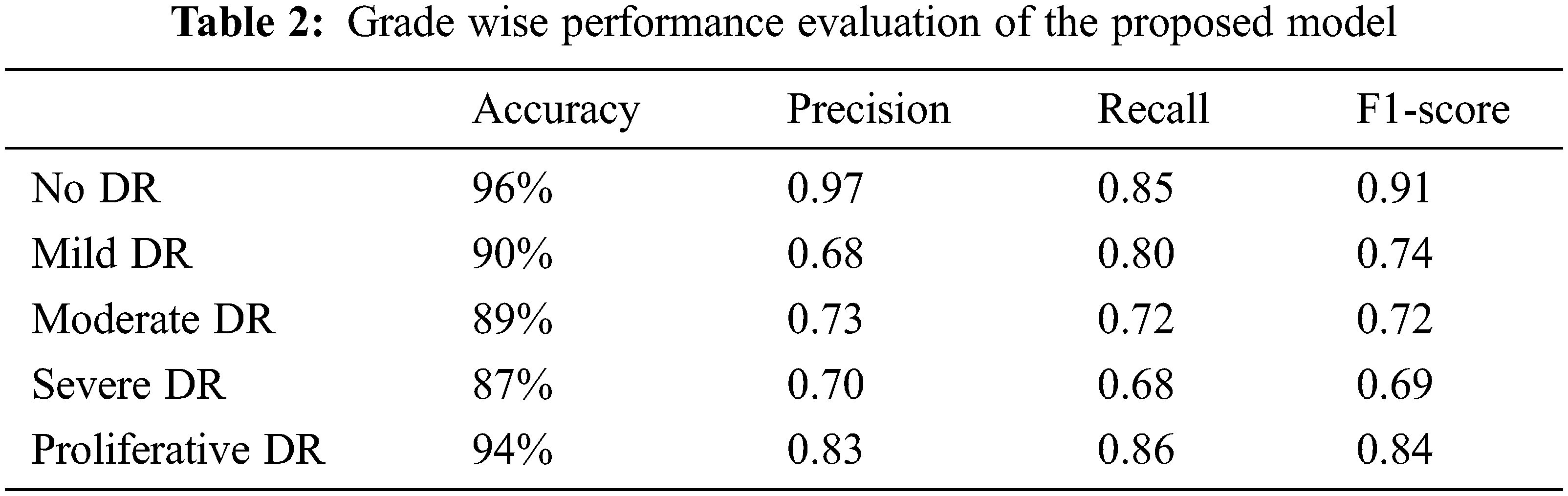
Hence, the average per-class accuracy which decides the per-class effectiveness of the classifier is 91.2%, and the Macro-average precision that decides the average per-class agreement of the true class labels with those of the classifier’s, the Macro-average recall that determines the average per-class effectiveness of a classifier to identify class labels, and the Macro-average F1-score that is the harmonic mean of micro-average precision and recall are 0.782, 0.782, and 0.780 respectively.

Fig. 9a represents the graph of training accuracy and testing accuracy for the grade wise DR classification. It shows the relation between accuracy and epoch for the Kaggle dataset. This graph runs for 50 epochs. The train and test accuracy were plotted and the model has achieved an overall accuracy of 91.2%. This shows that the model relatively worked well in determining the stages of Diabetic Retinopathy and classifying them to their respective categories, either as no DR, Mild, moderate, severe and Proliferative DR. Fig. 9b shows the training loss and testing loss for grade wise DR detection. The training loss achieved is 0.0831.

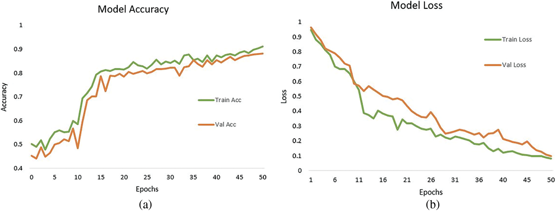
Figure 9: (a) Training accuracy and test accuracy of grade wise DR classification, (b) Training loss and test loss of grade wise DR classification

According to the research done before the proposed work, it is hard for the models to get a decent accuracy to detect Mild Diabetic Retinopathy images. In contrast, in this case, the model was able to do so. In addition, the advantage of combining resizing and augmentation into a single operation which has been done here, is that we do not have to interpolate the image multiple times, which typically degrades image quality.

4.7 Comparison of Classification Results with Existing Methods

Tab. 3 shows performance measurements of different operations performed by different researchers using the Kaggle dataset. The proposed model clearly shows that it achieved better results than all other models.

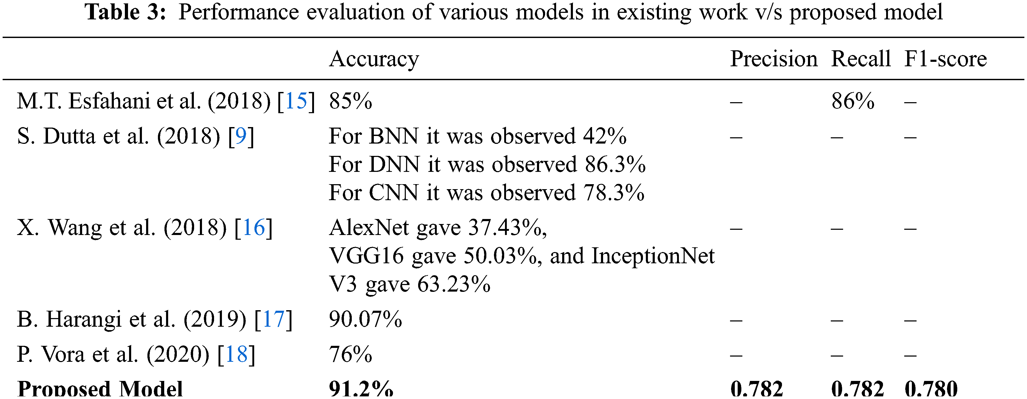
According to the research done before the proposed work, it is hard for the models to get a decent accuracy to detect Mild Diabetic Retinopathy images. In contrast, in this case, the model was able to do so. The advantage of combining resizing and augmentation into a single operation done here is that we do not have to interpolate the image multiple times, which typically degrades image quality. Furthermore, DenseNet is much more efficient in terms of parameters and computations to the same degree as ResNet and VGGNet. Therefore, the reuse of the gradient loss problem is facilitated, and the number of parameters is significantly reduced. Future work can include identifying and proposing machine learning/deep learning model frames that can reduce the existing overfitting, giving even better results on the test images. It will also include working with feature extraction like vessel segmentation, microaneurysm detection, and detection of hard and soft exudates, which will break down the problem of diabetic retinopathy, focussing on its symptoms in a very detailed manner. This will also help in the betterment of the performance of the model with improved time complexity.

5  Conclusion

Diabetic retinopathy is a critical public health issue affecting the quality of life. Patients receive specific treatment from a doctor to protect their vision to prevent the spread and progression of the disease. In the last few years, human beings have witnessed eye problems worldwide due to diabetes. Already existing DR uses manual fundus image analysis, which requires an experienced and skilled clinician to identify, detect, and analyze the presence and importance of the minor feature. It is also tedious and challenging. Here, three dense CNN models were proposed to detect DR according to disease severity and classify them into different classes. The proposed model contained various layers and parameters. Model 3 has come up with the best accuracy. The highest training accuracy achieved was 93.51%. The other two models have achieved maximum training accuracy of around 84% and 89%, respectively. The advantage of combining resizing and augmentation into a single operation done here is that we do not have to interpolate the image multiple times, which typically degrades image quality. The detection of mild and moderate DR is usually tricky, decently done by the proposed model. The data sets available for the proliferative phase are relatively small and pose a significant challenge. Therefore, training and classification are subject to the limited circumstances of the data set. The proposed model processed the processing time limit.

While there is a need to improve current accuracy, the presented results indicate a significant advance in diabetic retinopathy detection using computer vision to implement efficient software with lesser usage of resources and portable economical hardware. Thus, it can detect diabetic retinopathy without consulting an ophthalmologist in remote or medically inadequate locations and could significantly impact the relief of diabetes-based vision deterioration in the future.

Compliance with Ethical Standards

Acknowledgement: The authors would like to thank the SRM Institute of Science and Technology, Department of CSE for providing an excellent atmosphere for researching on this topic.

Funding Statement:The authors received no specific funding for this research.

Ethical Approval:This article does not contain any studies with human participants or animals performed by any of the authors.

Conflicts of Interest: The authors declare that they have no conflicts of interest to report regarding the present study.

References

1. J. Xu, X. Zhang, H. Chen, J. Li, J. Zhang et al., “Automatic analysis of microaneurysms turnover to diagnose the progression of diabetic retinopathy,” IEEE Access, vol. 6, pp. 9632–9642, 2018. [Google Scholar]
2. R. Pires, S. Avila, J. Wainer, E. Valle, M. D. Abramoff et al., “A data-driven approach to referable diabetic retinopathy detection,” Artificial Intelligence in Medicine, vol. 96, no. 6, pp. 93–106, 2019. [Google Scholar]
3. R. S. Rajkumar and A. G. Selvarani, “Diabetic retinopathy diagnosis using ResNet with fuzzy rough C-means clustering,” Computer Systems Science and Engineering, vol. 42, no. 2, pp. 509–521, 2022. [Google Scholar]
4. S. Sudha, A. Srinivasan and T. G. Devi, “Detection and classification of diabetic retinopathy using DCNN and BSN models,” CMC-Computers, Materials & Continua, vol. 72, no. 1, pp. 597–609, 2022. [Google Scholar]
5. S. Albahli and G. Nabi, “Detection of diabetic retinopathy using custom CNN to segment the lesions,” Intelligent Automation & Soft Computing, vol. 33, no. 2, pp. 837–853, 2022. [Google Scholar]
6. D. Sarwinda, T. Siswantining and A. Bustamam, “Classification of diabetic retinopathy stages using histogram of oriented gradients and shallow learning,” in 2018 Int. Conf. on Computer Control Informatics and it’s Applications (IC3INA), Tangerang, Indonesia, pp. 83–87, 2018. [Google Scholar]
7. P. Khojasteh, B. Aliahmad, S. P. Arjunan and D. K. Kumar, “Introducing a novel layer in convolutional neural network for automatic identification of diabetic retinopathy,” in 2018 40th Annual Int. Conf. of the IEEE Engineering in Medicine and Biology Society (EMBC), Berlin, Germany, pp. 5938–5941, 2018. [Google Scholar]
8. P. Costa, A. Galdran, A. Smailagic and A. Campilho, “A weakly-supervised framework for interpretable diabetic retinopathy detection on retinal images,” IEEE Access, vol. 6, pp. 18747–18758, 2018. [Google Scholar]
9. S. Dutta, B. Manideep, S. M. Basha, R. D. Caytiles and N. J. I. J. O. G. Iyengar, “Classification of diabetic retinopathy images by using deep learning models,” International Journal of Grid and Distributed Computing, vol. 11, no. 1, pp. 89–106, 2018. [Google Scholar]
10. S. Kumar and B. Kumar, “Diabetic retinopathy detection by extracting area and number of microaneurysm from colour fundus image,” in 2018 5th Int. Conf. on Signal Processing and Integrated Networks (SPIN), Amity University, Noida, pp. 359–364, 2018. [Google Scholar]
11. M. Mohsin Butt, G. Latif, D. N. F. Awang Iskandar, J. Alghazo and A. H. Khan, “Multi-channel convolutions neural network based diabetic retinopathy detection from fundus images,” Procedia Computer Science, vol. 163, no. 3, pp. 283–291, 2019. [Google Scholar]
12. Kaggle, “Detection-Detect diabetic retinopathy to stop blindness before it's too late”, Asia Pacific Tele-Ophthalmology Society (APTOS), 2019. [Online]. Available: https://www.kaggle.com/c/aptos2019-blindness-detection/overview/description. [Google Scholar]
13. Kaggle, “Diabetic retinopathy detection,” 2015. [Online]. Available: https://www.kaggle.com/c/diabetic-retinopathy-detection/overview. [Google Scholar]
14. G. Huang, Z. Liu, L. Van Der Maaten and K. Q. Weinberger, “Densely connected convolutional networks,” in 2017 IEEE Conf. on Computer Vision and Pattern Recognition (CVPR), Honolulu, HI, USA, pp. 2261–2269, 2017. [Google Scholar]
15. M. T. Esfahani, M. Ghaderi and R. J. L. E. J. P. T. Kafiyeh, “Classification of diabetic and normal fundus images using new deep learning method,” Leonardo Electronic Journal of Practices and Technologies, vol. 17, no. 32, pp. 233–248, 2018. [Google Scholar]
16. X. Wang, Y. Lu, Y. Wang and W.-B. Chen, “Diabetic retinopathy stage classification using convolutional neural networks,” in 2018 IEEE Int. Conf. on Information Reuse and Integration (IRI), Honolulu, HI, USA, pp. 465–471, 2018. [Google Scholar]
17. B. Harangi, J. Toth, A. Baran and A. Hajdu, “Automatic screening of fundus images using a combination of convolutional neural network and hand-crafted features,” in 2019 41st Annual Int. Conf. of the IEEE Engineering in Medicine and Biology Society (EMBC), Berlin, Germany, pp. 2699–2702, 2019. [Google Scholar]
18. P. Vora and S. J. A. S. Shrestha, “Detecting diabetic retinopathy using embedded computer vision,” Applied Sciences, vol. 10, no. 20, pp. 7274, 2020. [Google Scholar]
Cite This Article
Copyright © 2023 The Author(s). Published by Tech Science Press.
This work is licensed under a Creative Commons Attribution 4.0 International License , which permits unrestricted use, distribution, and reproduction in any medium, provided the original work is properly cited.
Downloads
Citation Tools