Optimal Dynamic Voltage Restorer Using Water Cycle Optimization Algorithm

1  Introduction

Nowadays, most of industrial equipment, for example, computing equipment, communication system, manufacturing process and robots are sensitive to voltage disturbances which requires high cost of maintenance [1]. Similarly, power quality (PQ) problems, such as voltage sag/swell, flicker, voltage unbalanced, harmonic current, etc have also been found to be common. Among the above-mentioned voltage-related problems, voltage sag and swell are the most frequent power quality problems [2,3]. Voltage sag occurs when the rms voltage drops by 10%–90% from the normal rated voltage and takes place for a half wave cycle to 1 min. Voltage sag is caused by the starting-up of large-power motors such as elevators, pumps, and air conditioning systems [4]. Voltage swell happens when the rms voltage exceeds the typical rated voltage by 110–180 percent; this takes a half-wave cycle to one minute. It usually happens when a large capacitive load is switched [5]. These power quality problems are presented in the IEEE 1159–2019 [6].

According to the literature, there are many common power devices which are used to improve power quality such as Unified Power Quality Conditioner (UPQC), Static Var Compensator (SVC), Dynamic Voltage Restorer (DVR), and Distribution Static Synchronous Compensator (D-STATCOM). However, DVR is the most effective and efficient approach for enhancing the voltage quality at load [7–9]. Many intelligent control schemes have been implemented in different DVR configurations to solve the power quality problems [10]. As reported in [11], a new control technique including the coupling of proportional and sequence-decouple resonant controllers is employed to provide more solutions for diverse scenarios. Additionally, a self-supported DVR scheme has been used with a grid-tied transformer for limiting fault currents [12]. The power grid is connected to a photovoltaic system as illustrated in [13] to improve power quality problems in an electricity system, including symmetrical/asymmetrical grid faults and voltage sags. In a wind system, a hybrid intelligent control is used in conjunction with DVR in [14] to show the fault ride through (FRT), and an artificial neural network (ANN) is used in conjunction with the ant-lion optimization technique in DVR to fix source-side voltage sag/swell under nonlinear loads conditions in [15]. In addition, a fuzzy logic-based DVR has been used with a PI controller to correct voltage sag/swell in [16], and a dual P–Q theory with an energy-optimized technique is implemented in DVR to minimize harmonics and solve voltage problems as described in [17]. Another simple and easy control technique used in DVR is the hysteresis band controller which has many variables switching frequency [18].

In the field of DVR, there are several studies that mentioned the implementation of DVR with different controller types, parameter optimization techniques and power quality issues as presented in Tab. 1. Based on Tab. 1, the proportional integral (PI) controller is commonly utilized with the controller gains optimized using arbitrary evolutionary metaheuristic techniques. However, this controller has a number of drawbacks, including the need for voltage and circuit detectors or sequence analyzers (positive/negative) circuits for current and voltage controllers, taking a long time to minimize small steady-state error and a high control effort [17,19]. Also, in this controller, some common power quality issues do not seem to have been addressed in the literature. ANN-based controller has been employed but it still suffers from the computational burden. FOPID is a candidate controller. Due to the fact that it has more parameters to be optimized, it could solve power quality issues more effectively when the appropriate optimization technique is employed [10]. Evolutionary metaheuristic algorithm is the nature-inspired optimization technique which has gained prominence in recent years with considerable success in various fields of application [20,21]. Water Cycle Algorithm (WCA) is one of the successful techniques for solving different constrained engineering problems in the literature [22–25]. It has never been used to find the optimal controller gain in the field of DVR. This paper therefore presents the comparison performances of the FOPID, FOPI, PID and PI controllers, of which the optimal controller gains are tuned by using the WCA evolutional metaheuristic optimization technique. The WCA searching results show its capability to find one set of controller gain which can solve all the power quality issues while the others in the literature need an individual set of optimal gain for each power quality problem. The comparative analysis of the results in the aspect of the DVR dynamic responses and total harmonic distortion (THD) are assessed and discussed. The results confirm the effectiveness of the proposed controller to solve balanced sag, balanced swell, unbalanced sag, and unbalanced swell power quality issues.

The rest of the paper starts with a presentation of the configuration of the DVR in Section 2. Then, the proposed control scheme of the DVR is introduced in Section 3. In Section 4, the fitness function, the formulation of the optimization problem and the detailed implementation of the optimization technique are illustrated. The simulation results and their corresponding comparative analysis of the different controllers are presented and discussed in Section 5. Finally, the conclusion is presented in Section 6.

2  Configurations of the System Under Study

The Dynamic Voltage Restorer (DVR) is a strong controller that is widely employed at the point of connection to mitigate voltage sags and swells [34,35]. The protected load is connected in series with the series voltage controller. A coupling transformer in series with the AC power source is commonly used to generate the compensation voltages. Depending on the compensation required, several types of energy storage can be used. Generally, the main components of DVR consist of a converter, a DC-link, a low pass LC filter and an injection transformer [36], as illustrated in Fig. 1. In this research, the parameters are designed as shown in Tab. 2.

Figure 1: Diagram of proposed dynamic voltage restorer (DVR)

3  The Proposed Control Scheme of the DVR

In the literature of fractional calculus [37,38], FOPID controllers are now widely used in many applications. The transfer function, which describes the structure of a common FOPID controller is shown in Eq. (1).

TFOPID(s)=KP+KIsλ+KDsμ) (1)

where Kp is the proportional gain; KI is the integral time constant gain, KD is the derivative time constant gain, λ is order of integration and µ is the order of differentiator. Proportional gain is used to improve on the dynamic response and the integral gain decreases steady state error whereas the derivative time constant gain improves the transient response by predicting the error that will occur in the future.

These parameters (Kp, KI, KD, λ and µ) can be optimized to obtain the optimal performance of the controller as shown in Fig. 2, depicting the implementation of the proposed method.

Figure 2: Implementation of the proposed method

The corresponding equations of the proposed compensation algorithm of DVR as shown in Fig. 2 are as follows [10]:

When the voltage disturbance occurs in the system, the reference voltages (Vref) are generated as shown in Eq. (2).

[Vref,aVref,bVref,c]=Vrated[sin⁡ωtsin⁡(ωt−2π3)sin⁡(ωt+2π3)] (2)

Then the reference voltages from Eq. (2) are transformed from three-phase abc-to-Dq0 components using the Park transformation technique as shown in Eq. (3).

[Vref,dVref,qVref,0]=23[cos⁡(ωt)cos⁡(ωt−2π3)cos⁡(ωt+2π3)−sin⁡(ωt)−sin⁡(ωt−2π3)−sin⁡(ωt−2π3)121212]×[Vref,aVref,bVref,c] (3)

Load voltages are measured and transformed from the three-phase abc-to-Dq0 using the Park transformation technique as shown in Eq. (4).

[VLoad,dVLoad,qVLoad,0]=23[cos⁡(ωt)cos⁡(ωt−2π3)cos⁡(ωt+2π3)−sin⁡(ωt)−sin⁡(ωt−2π3)−sin⁡(ωt−2π3)121212]×[VLoad,aVLoad,bVLoad,c] (4)

Dq0–reference voltages from Eq. (3) and Dq0-load voltages from Eq. (4) are compared to detect the error signal (et) as shown in Eq. (5).

|et,dq0|=(Vref,d−VLoad,d)2+(Vref,q−VLoad,q)2+(Vref,0−VLoad,0)2 (5)

Synchronization to the supply voltage is essential to regulate the inserted DVR adequately. This helps maintain the output signal of the controller in order to synchronize in frequency and phase with the reference input signal. A phase-locked loop (PLL) is applied in this study as a synchronization tool.

The error signal (et) from Eq. (5) is used to calculate ITAE value and optimal gains for all four proposed controllers are tuned using the Water cycle optimization techniques. The output of the controller (ut) is then transformed back to three-phase abc reference frame and the compensation voltages (VC,abc ) are generated as shown in Eq. (6).

[Vc,aVc,bVc,c]=[sin⁡(ωt)cos⁡(ωt)1sin⁡(ωt−2π3)cos⁡(ωt−2π3)1sin⁡(ωt+2π3)cos⁡(ωt+2π3)1]×[ut,dut,qut,0] (6)

The compensation voltages (VC,abc) were sent to the PWM generator to create the gating pulses for driving the three-leg voltage source inverter (VSI) which generated the compensating voltages to the system through the coupling transformers.

4  Formulation of the Optimization Problem

4.1 Fitness Function

In a common optimization problem, optimal gains of the controller are obtained by minimizing the objective function or sometimes also known as cost function. Optimization algorithm randomly generates a set of initial gain parameters and then computes the cost function for each set of parameters. In each iteration, this set of parameters is evoluted to obtain a minimum value of cost function. Several objective functions, e.g., integral absolute error (IAE), integral squared error (ISE), integral time absolute error (ITAE), have been reported in the literature to control problems but mostly ITAE is used for its superiority over the others. The mathematical formula of the ITAE is given in Eq. (7).

ITAE=∫0∞t|e(t)|dt (7)

4.2 Water Cycle Algorithm (WCA)

Water cycle algorithm (WCA) is a popular optimization technique introduced by H. Eskandar in 2012. The technique was inspired by the observation of water cycle and how river streams run down to the sea [39–41]. The raindrops are the initial population in WCA, and the problem controlled variables are denoted as xi .

The following equation is an example of how to define this array:

Raindrop=[x1,x2,x3,...,xN] (8)

The population of raindrops are genereted as the following equation:

PopulationofRaindrops={x1i:j=1:Npop and k=1:Nvar} (9)

where Npop denotes the number of raindrops and Nvar denotes the decision variables.

The Fitness functions of the raindrop are replaced by Ci which is gathered from

Ci=f(x1i,x2i,x3i,...,xNvari),i=1,2,3,...,Npop (10)

The best raindrops population is picked as the sea, the number of good raindrop population is chosen as rivers, and the remaining raindrops population is considered to be streams that run to the sea or rivers. Eq. (11) determines the streams that flow to a sea, or a river based on the intensity of the flow.

NSn=round{|Cn∑n=1NsrCn|×Npop},n=1,2,...,Nsr (11)

NSn is number of streams which flow into rivers or sea and Nsr is number of rivers and sea.

A stream flows to the river at a random distance (x) along the line that connects them [39]. The similar notion is used for rivers flowing to the sea, the new point for the streams and rivers can be described as:

Xstreami+1=Xstreami+rand×C×(Xriveri−Xstreami) (12)

Xriveri+1=Xriveri+rand×C×(Xseai−Xriveri) (13)

C is a constant value and it equals 1–2 where rand is the spread random numbers in the interval [0,1]

To prevent becoming locked in the local optimal, it is expected that an evaporation process will occur, clouds will form, and rain will commence (new random solutions). The condition in (14) is reviewed and if it is met, then, the evaporation process begins. dmax is a very small number near zero.

|Xseai−Xriveri|<dmax,i=1,2,3,...,Nsr−1 (14)

After each evaporation process, the value of dmax is as:

dmaxi+1=dmaxi−(dmaxi/maxiteration) (15)

After the evaporation phase, the raining process begins, and the new streams are formed because of the newly raindrops (random solution). Streams that flow directly to the sea as in the following equation are intended to increase stream production in order to enhance the best option for constrained issues.

Xstreamnew=Xsea+μ×ran(1,Nvar) (16)

μ is the coefficient that indicates the search range near the water and its value is usually equal to 0.1.

The flowchart of the proposed WCA technique can be found in [41].

4.3 Implementation of WCA Technique

Where J is the objective function and e is the error obtained by subtraction the plant output from set-point as shown in Fig. 3, WCA finds the optimal values of controller gains whose J has become minimum.

Figure 3: Implementation of WCA technique

The controller gains consist of Kp, Ki, Kd, λ and µ and the initial values of the WCA parameters are given below.

The maximum iteration (L) = 30;

The search agent size (N) = 50;

The lower boundary (lb) = 0.01;

The upper boundary (ub) = 30;

Number of variables (dim) = 5;

The maximum and minimum number of the decreasing factor Cmax = 1; Cmin = 0.0004

Tab. 3 shows the optimal gain values of the four controllers that are obtained from the WCA technique for correcting four cases of voltage disturbances, including, balanced sag, balanced swell, unbalanced sag and unbalanced swell as well as their corresponding ITAE values.

5  Results and Discussion

5.1 Modeling and Simulation

In MATLAB/Simulink platform, the proposed DVR is simulated in four cases below based on the arbitrary voltage disturbances, such as, balanced voltage sag and swell and unbalanced voltage sag and swell. In each case, the DVR is in the operation at the time interval t = 0.05 s – 0.2 s.

Case 1 Balanced voltage sag at 50% with respect to the reference voltage.

Case 2 Balanced voltage swell at 50% with respect to the reference voltage.

Case 3 Unbalanced voltage sag at phase A, B and C reduced to 80%, 70% and 50% with respect to the

reference voltage, respectively.

Case 4 Unbalanced voltage swell at phase A, B and C increased to 120%, 130% and 150% with respect to

the reference voltage, respectively.

The performance evaluation of optimal for the four controllers: PI, PID, FOPI and FOPID, are shown in Figs. 4–19.

Figure 4: Case 1 of PI Controller; (a) Supply voltage, compensating voltage and load voltage, (b) THD values of load voltage, (c) Rms voltage

Figure 5: Case 1 of PID Controller; (a) Supply voltage, compensating voltage and load voltage, (b) THD values of load voltage, (c) Rms voltage

Figure 6: Case 1 of FOPI Controller; (a) Supply voltage, compensating voltage and load voltage, (b) THD values of load voltage, (c) Rms voltage

Figure 7: Case 1 of FOPID Controller; (a) Supply voltage, compensating voltage and load voltage, (b) THD values of load voltage, (c) Rms voltage

Figure 8: Case 2 of PI Controller; (a) Supply voltage, compensating voltage and load voltage, (b) THD values of load voltage, (c) Rms voltage

Figure 9: Case 2 of PID Controller; (a) Supply voltage, compensating voltage and load voltage, (b) THD values of load voltage, (c) Rms voltage

Figure 10: Case 2 of FOPI Controller; (a) Supply voltage, compensating voltage and load voltage, (b) THD values of load voltage, (c) Rms voltage

Figure 11: Case 2 of FOPID Controller; (a) Supply voltage, compensating voltage and load voltage, (b) THD values of load voltage, (c) Rms voltage

Figure 12: Case 3 of PI Controller; (a) Supply voltage, compensating voltage and load voltage, (b) THD values of load voltage, (c) Rms voltage

Figure 13: Case 3 of PID Controller; (a) Supply voltage, compensating voltage and load voltage, (b) THD values of load voltage, (c) Rms voltage

Figure 14: Case 3 of FOPI Controller; (a) Supply voltage, compensating voltage and load voltage, (b) THD values of load voltage, (c) Rms voltage

Figure 15: Case 3 of FOPID Controller; (a) Supply voltage, compensating voltage and load voltage, (b) THD values of load voltage, (c) Rms voltage

Figure 16: Case 4 of PI Controller; (a) Supply voltage, compensating voltage and load voltage, (b) THD values of load voltage, (c) Rms voltage

Figure 17: Case 4 of PID Controller; (a) Supply voltage, compensating voltage and load voltage, (b) THD values of load voltage, (c) Rms voltage

Figure 18: Case 4 of FOPI Controller; (a) Supply voltage, compensating voltage and load voltage, (b) THD values of load voltage, (c) Rms voltage

Figure 19: Case 4 of FOPID Controller; (a) Supply voltage, compensating voltage and load voltage, (b) THD values of load voltage, (c) Rms voltage

5.1.1 Case 1: Three-Phase Balanced Voltage Sag

In case 1, the balanced voltage sag occurs at t = 0.05 − 0.2 s. It is found that PI, PID, FOPI and FOPID controllers are able to promptly compensate for the load voltage. For the PI controller, as shown in Fig. 4c, the compensated-load rms-voltages during the voltage sag yields the most different amplitude from the reference voltage at 18.63 V (8.47%) whereas the others restore the rms-load voltage nearly according to the reference voltage. Nevertheless, the PI controller could still restore the load voltage within the sensitive equipment voltage tolerance according to the Computer and Business Equipment Manufacturers Association (CBMEMA) curve [42].

The total harmonics distortions (THD) of the compensated load voltage from all the four controllers are less than 8% according to IEEE std. 519-2014 [6].

5.1.2 Case 2: Three-Phase Balanced Voltage Swell

In case 2, the Balanced voltage swell occurs at t = 0.05 − 0.2 s. It also shows that the PI controller, as seen in Fig. 8c, the compensated-load rms-voltage during voltage sag, yields different amplitude from the reference voltage at 9.83 V (4.47%). All four controllers were able to restore load voltages to the reference voltage within 1.35–1.62 Cycle (27.02–32.49 ms). The dynamic performance of all the controllers fall in the acceptable power quality area according to the CBEMA curve. The total harmonic distortion (THD) of the compensated load voltage from all the four controllers are within the 8% limit according to the IEEE std. 519-2014.

5.1.3 Case 3: Unbalanced Voltage Sag

In case 3, unbalanced voltage sag occurs at t = 0.05 − 0.2 s. It can be seen from the results that all four controllers can inject the necessary compensating voltages to keep the load voltages to their reference value and balance. They yielded the rapid dynamics response as seen from Figs. 12c, 13c, 14c and 15c; the rms-load voltages were almost promptly kept balance after the DVR was in operation.

5.1.4 Case 4: Unbalanced Voltage Swell

In case 4, unbalanced voltage swell occurs at t = 0.05 − 0.2 s. It shows that all four controllers can generate the compensating voltages to restore the load voltage to their reference value and keep balance within 1.27–1.64 cycle (25.47–32.80 ms). The dynamic responses of all the controllers fall in the acceptable power quality area according to the CBEMA curve. It further shows that the THD of the compensated load voltages from all four controllers are within the 8% limit according to the IEEE std. 519-2014.

5.2 Comparative Performance of the Controllers

5.2.1 Comparison from the Perspective of the Controller

As it can be seen from Tab. 3, the global error obtained by the WCA technique with the optimal PID controller (ITAEPID = 0.0117) is less than those obtained by the PI, FOPI, FOPID controllers (ITAEPI = ITAEFOPI = ITAEFOPID = 0.0153).

Tab. 4 illustrates the comparison of the controller performances in terms of response time and % steady-state error.

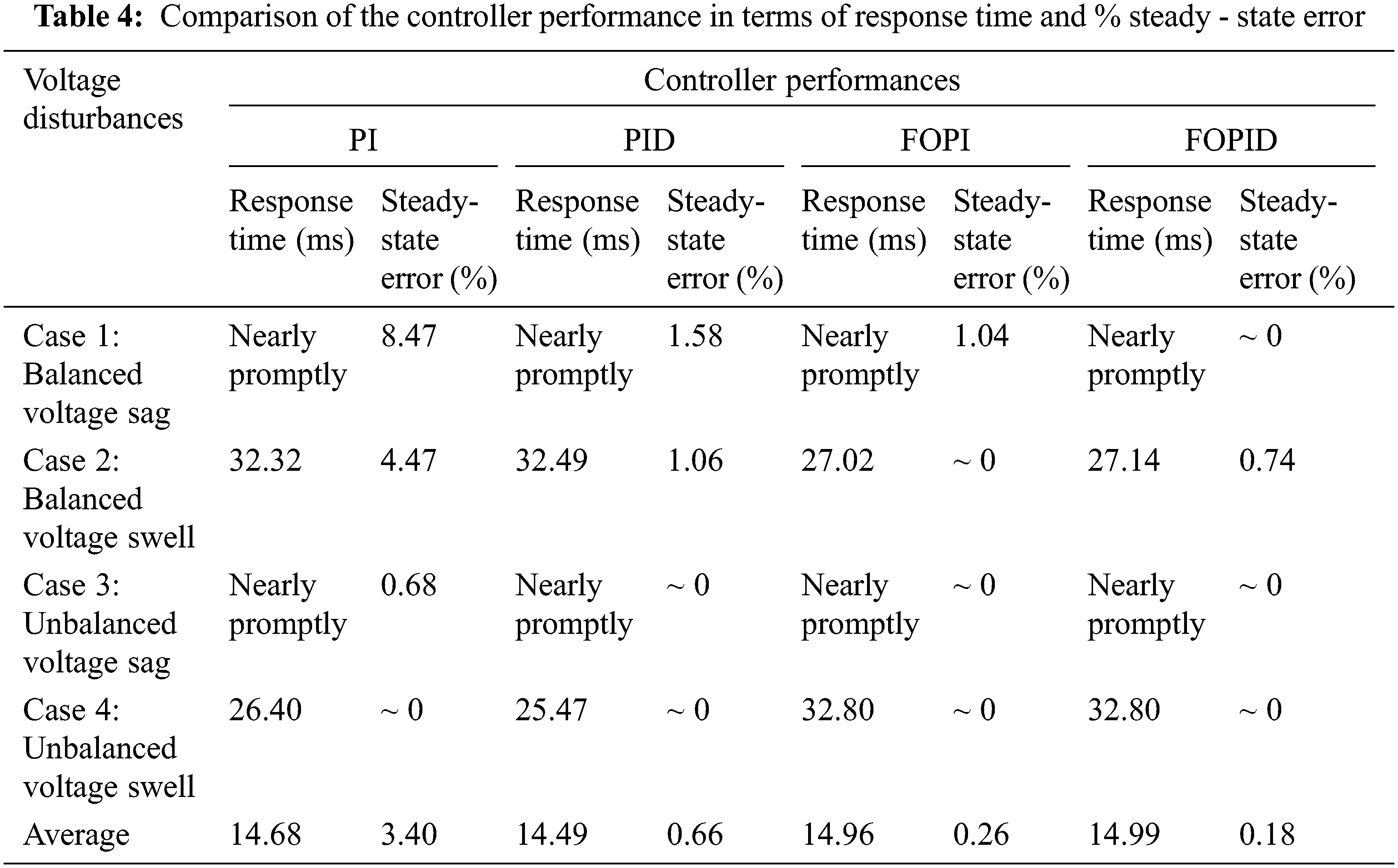
According to Tab. 4, the following aspects of response time include:

(1) In case 1 (Balanced voltage sag) and case 3 (Unbalanced voltage sag) voltage disturbances, all the controller yield the nearly promptly response time.

(2) In case 2 (Balanced voltage swell), FOPI and FOPID controllers yield faster response time (27.02 ms for FOPI and 27.14 ms for FOPID) compared to PI and PID controllers (32.32 ms for PI and 32.49 ms for PID). On the other hand, in case 4 (Unbalanced voltage swell), PI and PID yield faster response time (26.40 ms for PI and 25.47 ms for PID) compared to FOPI and FOPID controllers (32.80 ms for both FOPI and FOPID).

Tab. 4 also depicts from the average value that, in the aspect of response time, all controllers achieve a similar performance since the average response times of all the controllers are close to one another (14.49–14.99 ms). In the aspect of % steady-state error, FOPI and FOPID controllers (0.26% for FOPI and 0.18% for FOPID) are superior to PI and PID controller (3.40% for PI and 0.66% for PID). It should be noted that the % steady-state error of PI controller is significantly greater than the other controllers and the most inferior as well.

Still from Tab. 4, It can be observed from the aspect of % steady-state error that:

(1) In case 1 (Balanced voltage sag) and case 2 (Balanced voltage swell) voltage disturbances, PI controller yields the significant greatest % steady-state error compared to the others.

(2) In case 3 (Unbalanced sag) and case 4 (Unbalanced voltage swell) voltage disturbance, the % steady-state error obtained from all the controllers are not much different from one another and close to zero.

5.2.2 Comparison from the Perspective of the THD Results

Tab. 5 shows the comparison of the % THD content of the load voltages from each controller.

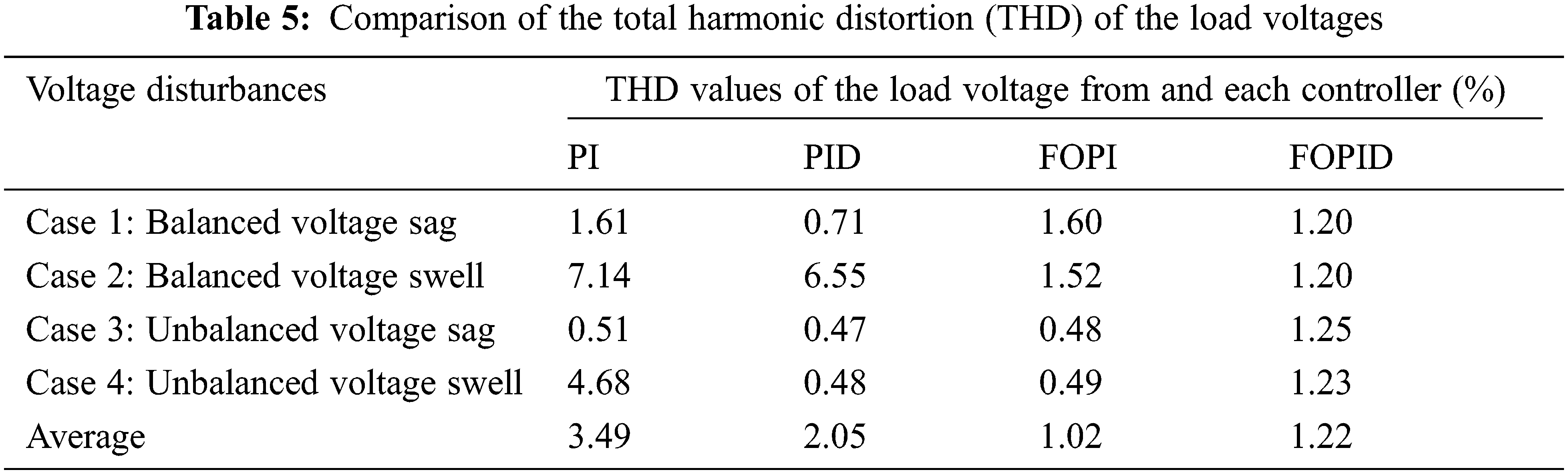
THD is a measurement used to evaluate harmonics distortion level in voltage or current waveforms [6]. According to IEEE standard 519-2014, THD should not exceed 8%. Higher level of harmonics can results in erratic, subtle break down, and other serious consequences [40]. As can be seen from the THD of load voltage in Tab. 5, it can be noted that:

(1) In case 1 (Balanced voltage sag), PID controller yields the lowest % THD compared to the others (THDPID = 0.71%, THDPI = 1.61%, THDFOPI = 1.60%, THDFOPID = 1.20%).

(2) In case 2 (Balanced voltage swell), PI, PID controllers yield the significant higher % THD (THDPI = 7.14%, THDPID = 6.55%) than those obtained from FOPI and FOPID controllers (THDFOPI = 1.52%, THDFOPID = 1.20%).

(3) In case 3 (Unbalanced voltage sag), FOPID controller yields the significant highest % THD (THDFOPID = 1.25%) compared to the others (THDPI = 0.51%, THDPID = 0.47%, THDFOPI = 0.48% ).

(4) In case 4 (Unbalanced voltage swell), PI controller yields the significant highest % THD compared to others with similarly low % THDs.

It is clearly seen from the average % THD value in Tab. 5 that the PI controller yields the highest average % THD value whereas FOPI controller yield the lowest.

To sum up from the comparison results, in term of average response time, the PID controller yields the most rapid performance (14.49 ms) while in term of average % steady-state error, the FOPID controller yields the lowest error percentage (0.18%). In the average % THD aspect, the FOPI controller yields the lowest THD percentage (1.02%). The least-effective performance controller is PI, which yields the greatest average steady-state error (3.40%) and THD (3.49%).

6  Conclusions

This paper presents a low complexity control scheme for voltage control of a dynamic voltage restorer (DVR) in three-phase system. The Water Cycle Algorithm technique (WCA) was applied to four controllers; PI, PID, FOPI and FOPID to search for the set of optimal controller gains which could be used to correct four main power quality problems: balanced voltage sags, balanced voltage swells, unbalanced voltage sag and unbalanced voltage swell. As shown in Tab. 1, WCA has not been previously applied to work with DVR to enhance power quality. Furthermore, WCA can find one set of optimum parameters that can be used for a wide range of problems and it can help to reduce the amount of computing time spent on correcting all the problems. Other methods in the literature have searched for different set of parameters for each case of the problem that are time consuming and inconvenient. Thus, the aforementioned result clearly shows the effectiveness of WCA in solving this problem.

The simulation results are discussed and compared in four cases of the above-mentioned power quality problems. The PID controller yields the most rapid performance in terms of average response time, FOPID controller yields the best performance in terms of average % steady-state error and the FOPI controller gives the lowest THD percentage in the average %THD aspect. However, the FOPID result did not differ much in average response from the PID (PID 14.49 ms/FOPID 14.99 ms) and average % THD from FOPI (FOPI 1.02%/FOPID 1.22%). Yet, FOPID yields the most outstanding average steady-state error at 0.18%. From the results, it is found that the dynamic responses of all controllers fall in the acceptable power quality area according to the CBMA curve. The total harmonic distortion (THD) of the compensated load voltage from all controllers are within the 8% limit in accordance to the IEEE std. 519-2014.

Funding Statement: This Research was Financially Supported by Faculty of Engineering, Mahasarakham University (Grant year 2021).

Conflicts of Interest: The authors declare that they have no conflicts of interest to report regarding the present study.

References

1. R. S. Vedam and M. S. Sarma, Power Quality: VAR Compensation in Power Systems, 1st ed., CRC press, Florida, U. S. A., 2009. [Google Scholar]
2. J. Martinez and J. M. Jacinto, “Voltage sag studies in distribution networks—part I: System modeling,” IEEE Transaction on Power Delivery, vol. 21, no. 3, pp. 1670–1678, 2006. [Google Scholar]
3. M. G. Simes and F. A. Farret, Power quality analysis. In: Modeling Power Electronics and Interfacing Energy Conversion Systems, 1st ed., NJ, USA: John Wiley & Sons, pp. 227–253, 2017. [Google Scholar]
4. K. S. Arash and K. M. Smedley, “Fast and precise voltage sag detection method for dynamic voltage restorer (DVR) application,” Electric Power Systems Research, vol. 130, pp. 192–207, 2016. [Google Scholar]
5. E. A. Nagata, D. D. Ferreira, C. A. Duque and A. S. Cequira, “Voltage sag and swell detection and segmentation based on independent component analysis,” Electric Power Systems Research, vol. 155, pp. 274–280, 2018. [Google Scholar]
6. IEEE Standards Association, “IEEE recommended practice for monitoring electric power quality,” IEEE Standard 1159–2019, 2019. [Google Scholar]
7. P. Kanjiya, B. Singh, A. Chandra and L. Al-Haddad, “SRF theory revisited to control self-supported dynamic voltage restorer (DVR) for unbalanced and nonlinear loads,” IEEE Transactions on Industry Applications, vol. 49, no. 5, pp. 2330–2340, 2017. [Google Scholar]
8. D. Saeed, M. Shahparasti, M. Simab and S. M. Mortazavi, “Employing interface compensators to enhance the power quality in hybrid AC/DC microgrids,” Ciência e Natura, vol. 37, no. 6–2, pp. 357–363, 2015. [Google Scholar]
9. M. Khiat Benali, T. Allaoui and M. Denaï, “Power quality improvement and low voltage ride through capability in hybrid wind-PV farms grid-connected using dynamic voltage restorer,” IEEE Access, vol. 6, no. 1, pp. 68634–68648, 2018. [Google Scholar]
10. A. Omar, S. H. Aleem, E. E. El-Zahab, M. Algeblawy and Z. M. Ali, “An improved approach for robust control of dynamic voltage restorer and power quality enhancement using grasshopper optimization algorithm,” ISA Transaction, vol. 95, pp. 110–129, 2019. [Google Scholar]
11. D. V. Tien, R. Gono and L. Zbigniew, “A multifunctional dynamic voltage restorer for power quality improvement,” Energies, vol. 11, no. 6, pp. 1351–1368, 2018. [Google Scholar]
12. H. Nourmohamadi, S. I. Bektas, S. H. Hosseini, E. Babaei and M. Sabahi, “A conventional dynamic voltage restorer with fault current limiting capability,” Procedia Computer Science, vol. 120, pp. 750–757, 2017. [Google Scholar]
13. A. M. Rauf and V. Khadkikar, “Integrated photovoltaic and dynamic voltage restorer system configuration,” IEEE Transactions on Sustainable Energy, vol. 6, no. 2, pp. 400–410, 2015. [Google Scholar]
14. R. Sitharan, C. K. Sundarabalan, K. R. Devebalaji, S. K. Nataraj and M. Karthikeyan, “Improved fault ride through capability of DFIG-wind turbines using customized dynamic voltage restorer,” Sustainable Cities and Society, vol. 39, no. no. 2, pp. 114–125, 2018. [Google Scholar]
15. V. Ansal, “ALO-optimized artificial neural network-controlled dynamic voltage restorer for compensation of voltage issues in distribution system,” Soft Computing, vol. 24, no. 1, pp. 1171–1184, 2019. [Google Scholar]
16. M. T. Hagh, A. Shaker, F. Sohrabi and I. S. Gunsel, “Fuzzy-based controller for DVR in the presence of DG,” Procedia Computer Science, vol. 120, no. 11, pp. 684–690, 2017. [Google Scholar]
17. M. Pradhan and M. K. Mishra, “Dual P-Q theory-based energy-optimized dynamic voltage restorer for power quality improvement in a distribution system,” IEEE Transactions on Industrial Electronics, vol. 66, no. 4, pp. 2946–2955, 2018. [Google Scholar]
18. S. Sasitharan and M. K. Mishra, “Constant switching frequency band controller for dynamic voltage restorer,” IET Power Electronics, vol. 3, no. 5, pp. 657–667, 2010. [Google Scholar]
19. H. R. Hafezi and R. Faranda, “Dynamic voltage conditioner: A new concept for smart low-voltage distribution systems,” IEEE Transactions on Power Electronics, vol. 33, no. 9, pp. 7582–7590, 2018. [Google Scholar]
20. D. Greiner, J. Periaux, D. Quagliarella, J. Magalhaes-Mendes and B. Galván, “Evolutionary algorithms and metaheuristics: Applications in engineering design and optimization,” Mathematical Problems in Engineering, vol. 2018, pp. 1–4, 2018. [Google Scholar]
21. X. R. Zhang, W. F. Zhang, W. Sun, X. M. Sun and S. K. Jha, “A robust 3-D medical watermarking based on wavelet transform for data protection,” Computer Systems Science & Engineering, vol. 41, no. 3, pp. 1043–1056, 2022. [Google Scholar]
22. A. Latif, D. C. Das, S. Ranjan and A. K. Barik, “Comparative performance evaluation of WCA-optimised non- integer controller employed with WPG-DSPG–PHEV based isolated two-area interconnected microgrid system,” IET Renewable Power Generation, vol. 13, no. 5, pp. 725–736, 2019. [Google Scholar]
23. A. Sadollah, H. Eskandar, A. Bahreininejad and J. H. Kim, “Water cycle, mine blast and improved mine blast algorithms for discrete sizing optimization of truss structures,” Computers & Structures, vol. 149, no. 5, pp. 1–16, 2015. [Google Scholar]
24. M. A. Elhameed and A. A. El-Fergany, “Water cycle algorithm-based load frequency controller for interconnected power systems comprising nonlinearity,” IET Generation, Transmission & Distribution, vol. 10, no. 15, pp. 3950–3961, 2016. [Google Scholar]
25. M. A. Elhameed and A. A. El-Fergany, “Water cycle algorithm-based economic dispatcher for sequential and simultaneous objectives including practical constraints,” Applied Soft Computing, vol. 58, no. 3, pp. 145–154, 2017. [Google Scholar]
26. T. A. Naidu, S. R. Arya and R. Maurya, “Multi-objective dynamic voltage restorer with modified EPLL control and optimized PI controller gains,” IEEE Transactions on Power Electronics, vol. 34, no. 3, pp. 2181–2192, 2018. [Google Scholar]
27. T. A. Naidu, S. R. Arya and R. Maurya, “Dynamic voltage restorer with quasi-Newton filter-based control algorithm and optimized values of PI regulator gains,” IEEE Journal of Emerging and Selected Topics in Power Electronics, vol. 7, no. 4, pp. 2476–2485, 2019. [Google Scholar]
28. F. Jiang, C. Tu, Q. Guo, Z. Shuai, X. He et al., “Dual-functional dynamic voltage restorer to limit fault current,” IEEE Transactions on Power Electronics, vol. 66, no. 7, pp. 5300–5309, 2019. [Google Scholar]
29. L. R. Merchan-Villalba, J. M. Lozano-Garcia, J. G. Avina-Cervantes, H. J. Estrada-Garcia, A. Pizano-Martinez et al., “Linearly decoupled control of a dynamic voltage restorer without energy storage,” Mathematical Modeling in Industrial Engineering and Electrical Engineering, vol. 8, no. 10, pp. 1–18, 2020. [Google Scholar]
30. E. Molla and C. Kuo, “Voltage sag enhancement of grid connected hybrid PV-wind power system using battery and SMES based dynamic voltage restorer,” IEEE Access, vol. 8, pp. 130003–130013, 2020. [Google Scholar]
31. Z. Elkady, N. Abdel-Rahim, A. Mansour and F. Bendary, “Enhanced DVR control system based on the Harris Hawks optimization algorithm,” IEEE Access, vol. 8, pp. 177721– 177733, 2020. [Google Scholar]
32. S. C. Yáñez-Campos, G. Cerda-Villafaña and J. M. Lozano-García, “A two-grid interline dynamic voltage restorer based on two three-phase input matrix converters,” Applied Sciences, vol. 11, no. 2, pp. 561–586, 2021. [Google Scholar]
33. T. A. Naidu, S. R. Arya, R. Maurya and P. Sanjeevikumar, “Performance of DVR using optimized PI controller based gradient adaptive variable step LMS control algorithm,” IEEE Journal of Emerging and Selected Topics in Industrial Electronics, vol. 2, no. 2, pp. 155–163, 2021. [Google Scholar]
34. K. Chan and A. Kara, “Voltage sags mitigation with an integrated gate commutated thyristor based dynamic voltage restorer,” in Proc. of 8th ICHQP, Athens, Greece, pp. 210–215, 1998. [Google Scholar]
35. S. S. Choi, B. H. Li and D. D. Vilathgamuwa, “Dynamic voltage restoration with minimum energy injection,” IEEE Transactions on Power Systems, vol. 15, no. 1, pp. 51–57, 2000. [Google Scholar]
36. H. Kim and S. K. Sul, “Compensation voltage control in dynamic voltage restorers by use of feed forward and state feedback scheme,” IEEE Transactions on Power Systems, vol. 20, no. 5, pp. 1169–1177, 2005. [Google Scholar]
37. P. Shah and S. Agashe, “Review of fractional PID controller,” Mechatronics, vol. 38, no. 7, pp. 29–41, 2016. [Google Scholar]
38. N. X. Liu and J. T. Fei, “Fractional-order PID and active disturbance rejection control for active power,” in Proc. 29th Chinese Control and Decision Conf. (CCDC), Chongqing, China, pp. 2678–2683, 2017. [Google Scholar]
39. H. Eskandara, A. Sadollahb, A. Bahreininejadb and M. Hamdib, “Water cycle algorithm-a novel metaheuristic optimization method for solving constrained engineering optimization problems,” Computer & Structures, vol. 110, no. 1, pp. 151–166, 2012. [Google Scholar]
40. A. Sadollah, H. Eskandar, H. Lee, D. G. Yoo and J. H. Kim, “Water cycle algorithm: A detailed standard code,” SoftwareX, vol. 5, no. 1, pp. 37–43, 2016. [Google Scholar]
41. A. A. A. El-Ela, R. A. El-Sehiemy and A. S. Abbas, “Optimal placement and sizing of distributed generation and capacitor banks in distribution systems using water cycle algorithm,” IEEE Systems Journal, vol. 12, no. 4, pp. 3629–3636, 2018. [Google Scholar]
42. J. Kyei, R. Ayyanar, G. Heydt, R. Thallam and J. Blevins, “The design of power acceptability curves,” IEEE Transactions on Power Delivery, vol. 17, no. 3, pp. 828–833, 2002. [Google Scholar]
Cite This Article
Copyright © 2023 The Author(s). Published by Tech Science Press.
This work is licensed under a Creative Commons Attribution 4.0 International License , which permits unrestricted use, distribution, and reproduction in any medium, provided the original work is properly cited.
Downloads
Citation Tools