Predictive-Analysis-based Machine Learning Model for Fraud Detection with Boosting Classifiers

1  Introduction

Online transactions have been prevalent the Indian as well as world-wide market substantially. As a result, the worldwide E-Commerce market is expected to grow at a rapid pace, reaching $4.9 trillion by 2021. This surely prompts criminals to look for ways to access victims’ wallets via the Internet [1]. It is anticipated to grow to $106 billion by 2027, according to the data from Fortune Business Insights. The increasing number of transactions in the duration of the COVID-19 lockdowns could push this figure much higher than expected. Money laundering, insurance claims and electronic payments will account for the largest portions for the detection and prevention of these sharp practices by 2021 [2].

Credit default occurs when a client fails to meet the legal responsibilities or terms of a loan as stated in the promissory note. In other words, loan or credit default occurs when a borrower fails to repay a loan according to the terms agreed to prior to the loan’s acceptance. A non-performing loan is one in which a borrower has taken out a specified amount of credit but has failed to repay it in the agreed-upon time frame of 90 days for commercial banking loans and 180 days for consumer loans. Nonpayment means that, depending on the type of loan, purpose, or industry, neither the interest nor the principle on that credit is paid in 90 to 180 days. Any definition of a non-performing loan is based on the loan’s conditions and the existing agreement, as the definition is conditional and based on promissory notes and agreements.

Various banks have conducted forensic audits in the recent past, either on the orders of the RBI (Reserve Bank of India) or on their own initiative. The Reserve Bank of India has issued guidelines for classifying and reporting frauds. It has also established a standardised provisioning standard for all incidents of fraud. The current wave of financial frauds, on the other hand, shows no indications of slowing down. This, combined with delays in detection and reporting, is exacerbating the problem, as information is not shared with other institutions in a timely manner to prevent problems from arising. The Reserve Bank of India has increasingly increased its focus on borrowers’ bank frauds and has established several procedures to mitigate this risk over time.

To cope with loan frauds with exposures of more than INR(Indian Rupee) 50 crore, the new concept of a “Red Flagged Account” (RFA) has been added into the existing fraud risk management system. The RFA must proactively identify loan accounts that have Early Warning Signals (EWS) or typical‘red flag(s)’ (a phrase used to describe any aberration, aberrant pattern, or warning signal). A bank is expected to examine such signals over a predetermined time period in order to establish the incidence of fraud, if any, and to report it to the RBI appropriately.

Other than these approaches, machine learning is also frequently being implemented as a machine learning is the use of a combination of computer algorithms and statistical modeling to allow a computer to accomplish tasks without the need for hard coding [3,4]. These algorithms are gradually appearing to be more effective when it comes to the speed with which information is processed these days. The performance of various machine learning techniques such as Decision Tree, Random Forest, linear regression, and Gradient Boosting Method for detecting and predicting fraud instances utilizing loan fraudulent manifestations is compared in this research.

1.1 Literature Survey

Anomaly detection in different frauds is the subject of multiple survey articles that provide a good overview of current trends. Ngai et al. [5] provided an early thorough investigation of intelligent systems for financial fraud detection. The survey conducted by Ahmed et al. [6] provides an overview of anomaly detection approaches in the financial domain, specifically clustering algorithms. Following that, Ahmed et al. [7] outlined assumptions for detecting anomalies and summarized research using partition-based and hierarchical-based clustering techniques. A survey on fraud detection systems was proposed by Abdallah et al. [8]. Furthermore, Gai et al. [9] suggested a very thorough survey on Fintech technology in general, while Ryman-Tubb et al. [10] proposed a study on credit card fraud detection. The survey results of applying classification algorithms to financial fraud detection were then presented by West et al. [11]. Pourhabib et al. [12] provided a general overview of graph-based anomaly detection algorithms. Long short-term memory (LSTM) is another strategy that has recently been researched in the Fintech industry [13,14].

Credit card fraud, telecommunication fraud, computer intrusion, bankruptcy fraud, theft fraud or counterfeit fraud, and application frau13d are all examples of fraud, according to [15]. The impact of fraud on a country’s economy is real, and various measures have been tried, yet they all have flaws. Machine learning, on the other hand, has proven to be more dependable. Machine learning employs data mining techniques to uncover hidden patterns in big, volatile, and diverse datasets, allowing users to make informed decisions based on the information gained. A high rate of default has been documented in several countries, and this can be lowered through the use of information technology.

Using tree structure techniques, the decision tree divides data into distinct categories [16–18]. It classifies from the root to the leaf node and highlights the structural information in the data [19]. The simplicity and speed of decision trees are unrivalled; there is no requirement for domain knowledge or parameter setting; it also comfortably handles high dimensional data with many attributes; the way it is represented allows for enhanced comprehensibility; it has fantastic accuracy, though this is dependent on the data in use; it supports incremental learning; they are unvarried, simplifications. They operate well for both classification and regression issues; they can manage missing information; trees are graphically shown and easily interpreted; and, perhaps most importantly, trees are simple to explain to people [20,21].

Maes et al. [22] discussed numerous fraud detection issues. First, training efficient models is difficult due to the highly unbalanced datasets in this application, where only a small percentage of the available data is fraud. Zareapoor et al. [23] released a work on Fraud Detection using Naive Bayes, KNN(K-Nearest Neighbors), SVM (Support Vector Machine), and Bagging Ensemble Classifier Techniques. The study Credit card fraud detection using AdaBoost by Randhawa et al. [24] examines a variety of machine learning techniques, including Nave Bayes, Random Forest, Gradient Boosted Tree, and others. They employ “Majority voting” to combine two or more algorithms in this study. The study also looks into the AdaBoost ensemble model, finding that it is extremely susceptible to anomalies and outliers.

In an unsupervised learning scenario, restricted Boltzmann machines (RBM) can be utilized for data reconstruction. In their paper [25], Pumsirirat and Yan employed Keras to implement this high-level neural network. They calculated the Mean Squared Error, Root Mean Square Error, and Variable Importance of the attributes in each dataset using the H2O package. For each scenario, Keras was used to calculate the Area under the Curve (AUC) and Confusion Matrixes. AutoEncoders are described by Tom Sweers in his bachelor thesis [26] as an effective neural network that can encode data while learning to decode it. In this method, autoencoders are trained on non-anomaly points and then introduced to anomaly points to categorize them as “fraud” or “no fraud” based on the reconstruction error, which is expected to be large in the case of anomalies on which the system has not been taught. This method was also utilized in the publication Autoencoder-based network anomaly detection by Chen et al. [27].

Magomedov et al. [28] suggested a fraud management anomaly detection approach based on machine learning and graph databases. Huang et al. [29] presented a work with the same purpose and an emphasis on money laundering. They developed CoDetect, a detection system that analyses a network, including its entities and transactions, and then discovers frauds and feature patterns. For many real-world fraud scenarios, CoDetect employs a graph mining approach. Amarasinghe et al. [30] presented another general discussion on the use of machine learning for fraud detection in financial transactions

1.2 Dataset

The data has been collected from the Lending Club website (https://www.lendingclub.com/). Lending Club is an American company located in San Francisco, California. The company provides online platform for the investors and borrowers. Lending Club takes fees from both borrowers and investors for processing the loans. Till December 2015, a total of $15.98 billion has been given as loans through this platform.

1.3 Problem Statement

Number of machine learning algorithms has been applied for fraud detection and prediction in various cases such as loan, credit/debit cards, etc. It is also obvious from the literature review that no algorithm may be equally performing on all types of datasets. So here in this paper, a comparative study has been performed on loan fraud detection and prediction with the machine leaning algorithms such as Decision Tree, Random Forest, linear regression, and Gradient Boosting Methods. Further model accuracy metric have been conducted with confusion matrix and calculation of accuracy, precision, recall and F-1 score along with ROC curves.

2  Machine Learning Algorithms

2.1 Random Forest and Decision Tree

The random forest was first created by tin kam ho in 1995 by applying random space technique, which was proposed by ho in the stochastic discrimination approach for the classification problem coined by Eugene Kleinberg [31,32]. It considers those trees which selects most of the class values. In the case of regression, the mean or average values of the dependent variable are reflected by different decision trees from the random forest [33,34]. Random forests are generally applied to rectify the problem of overfitting while training the model with data [35,36].

Eugene Kleinberg proposed the “Stochastic Discrimination” method for classification in 1990 [37], and Tin Kam Ho introduced Random Decision Forest utilizing the Random subspace approach in 1995, in which Tin Kam Ho employed Eugene Kleinberg’s “Stochastic Discrimination.” The Random subspace approach removes the correlation between the trees and improves the accuracy of the final model by stochastically selecting a subset of observations and variables from the original data [38]. Later, Leo Breiman and Adele Culter extended Kam Ho’s technique by combining the concepts of “Bagging” or “Bootstrap Aggregation” with “Random Selection of Variables” and trade marking the term “Random Forests [39].” Both qualitative and quantitative dependent variables can be predicted using the Random Forest approach.

The Bias-Variance tread off is the fundamental disadvantage of the Random Forest approach. When we increase the depth of the trees, the bias decreases, but the model tends to over fit, resulting in high variance when predicting with new data; conversely, when we lower the depth of the tree, the model suffers from high bias [40].

A decision tree is a hierarchical model for the supervised learning. A decision tree is composed of inter decision nodes and terminal layers. Each decision node ‘m’ implements a test function fm(x) with discrete outcomes which are called the branches. In Fig. 1, a decision tree splits the data set in order to classify the squares and circles.

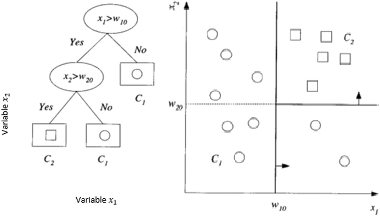
Figure 1: Showing dataset split in the decision tree process

In above diagram, the dataset split rules is elaborated. The first variable x1 has been considered to split the dataset, and the rule to split the dataset was x1>w10 and further, the dataset was divided into two based on the variable x2 and the rule was x2>w20 . By comparing the input dataset and the decision tree rules, it is observed that after the final split, the leaves have only one category either circle or square. Finally, if any observation satisfies the rule x1>w10andx2>w20 then it is a class c2 otherwise, it is a class c1 . The obvious question here is ‘how to decide the variable and the split rule? ’

There are two types of splits in a decision tree namely, a pure split and an impure split. The purity of the split is quantified by the calculation of an impurity measure; if all the observations in a resultant split are same then it is called as a pure split. In Fig. 1. the second split rule x2>w20 is a pure split, because in the final split we have only c1 in the first branch and only c2 in the second branch. If the split is a pure split, then no need to split the node further we can leave it as a final leaf node.

There are three popular impurity measures namely, Entropy, Gini Index and Miss-Classification error to split the decision tree.

Entropy=ϕ(p,1−p)=−log2p−(1−p)log2(1−p) (1)

GiniIndex=∅(p,1−p)=2p(1−p) (2)

MissClassificationError=GiniIndex=ϕ(p,1−p)=1−maxp(1−p) (3)

Here p is the probability to select the class c1 and (1−p) is the probability to consider c2 . In the decision tree process, first the entropy is calculated for all the variables and the variable is selected with maximum entropy because if the variable with maximum impurity is considered then the number of steps to reach the purity will be the minimum.

2.2 Gradient Boosting Ensemble Learning Technique

However India have been going through online transactions from last many years, but in the second tenure of the current prime minister, digital transaction has been more frequently opted media for sending and receiving money instantaneously. Transactions are being conducted through online banking, debit and credit cards, UPIs and many more. A credit card enables digital transaction more convenient and frequent since it provides many facilities. It is generally issued by different banks and works on the concept “use now pay later” basis for buying goods at offline stores, and even while purchasing many things in online mode, etc. [41]. Since it hardly asks for any authentication, it’s misused very frequently when lost or stolen.

Between the month of April and December, 2018, around 24,000 were registered related to debit and credit card fraud including internet banking in India. Alone in the Mumbai only, 42% cases out of total cases were registered in 2017, the newspaper, Hindustan Times report. In the year 2016, as per a report published by Global Consumer Fraud agency, India has been noticed as 5th position in the world with respect to credit card, debit card, UPI, and internet banking transactions [42,43].

Gradient boosting algorithm is considered under machine learning technique applied for classification and regression for developing prediction models by constituting weak prediction models such as decision trees [44]. In the case of weak decision tree learner, the performing decision trees are called as gradient boosted trees, which may better perform than random forest [45]. It develops the model which performs in state-wise manner such as boosting technique does, and also brings about generalization by permitting optimization of an arbitrarily differentiable error function [46,47]. The model assigns weights to all of the parameters at random in the first phase and predicts the outcomes. It will calculate the errors based on the initial predictions, and then apply the Gradient Descent to determine how much we need to adjust the parameters to further reduce the error [48,49].

Random forest has been performing quite remarkably on the huge and unbalanced dataset [50]. There are obvious reasons for getting unbalanced dataset in this context. Since there very much unbalanced datasets it becomes quite challenging to learn with such data [51,52] and it leads to unexpected performance of algorithms such as SVM or Random forest [53,54]. In fact, imbalanced class data have been representing to produce unexpected results on the performance of a wide variety of classifiers [55]. Skewed class data distributions also affect with the negative performance in the case of decision trees and neural networks [56]. K-Nearest Neighbors algorithm has also not been performing well with imbalanced datasets Overall, most of the classifiers suffer from class imbalance, some more than others [57].

One of the most popular and accurate ensemble learning techniques created in the last two decades is gradient boosting. Gradient Boosting is a machine learning technique for regression and classification problems that generates a prediction model from an ensemble of weak prediction models, usually decision trees [58].

The fundamental magic of all machine learning models is gradient descent. The Gradient Descent is an iterative technique that aims to find the error function’s minimum value [59]. The Gradient Descent formula can be found in the following Eq. (4).

W1=W0−α∗∇J(W) (4)

Here W0 is the initial error value, ∇ is the direction of the step, J(W) is the magnitude of the direction evaluated at W0 and α is the step size also known as Learning Rate [60].

Let’s examine the process with a simple straight-line example,

y=α+βX (5)

Here α is the intercept parameter and β is the slope parameter of the equation. Now let us consider Mean sum of squares as the error function, which can be written as

J(W)=1N∑i=1N(yi′−y^i′)2 (6)

Here y^i′s are the predicted values and yi′s are the actual values. Now if the errors are calculated for various values of yi′ , a graph could be plotted as in the following Fig. 1. Further the slope of the curve is calculated at any point using the derivatives. Since there are two parameters α and β , it needs to minimize the function with respect to both α and β.

Differentiating the Eq. (6) with respect to the intercept parameter α, we get

dj(w)dα=ddα1N∑i=1N(yi′−y^i′)2

=ddα1N∑i=1N(yi′−(α+βXi))2

=2N∑i=1N(yi′−(α+βXi))(−1) (7)

Now, by solving the Eq. (7), the value of the intercept α could be achieved, at which, the error function is minimum. By using gradient descent method also, it could be solved the equation for a minimum value [61]. After solving the equation, update the initial arbitrary value with the new intercept using Eq. (4).

Differentiating with respect to the slope parameter β

dj(w)dβ=ddβ1N∑i=1N(yi′−y^i′)2

=ddβ1N∑i=1N(yi′−(α+βXi))2

=2N∑i=1N(yi′−(α+βXi))−Xi (8)

By solving the Eq. (5) the value of β could be achieved. Same as intercept α , it can update the slope coefficient β and get the new estimates for β .

The steps in the Gradient Descent Model are given as follows:

Input Data {(xi,yi)}i=1n and a differentiable Loss Function L(yi,f(xi))

Step 1: Initialize f0(x)=argminγ∑i=1NL(yi,γ)

Step 2: For m = 1 to M:

a) For I = 1,2, …, N, compute, γim=−[∂L(yi,f(xi))∂f(xi)]f(x)=fm−1(x)

b) Fit a Decision Tree to the targets γim giving terminal regions RJm;j=1,2,3,…,Jm

c) For j=1,2,3,…,Jm compute, γim=argmin(γ)∑xi∈RJmL(yi,fm−1(xi)+γ)

d) Update fm(x)=fm−1(x)+∑j=1jmγmI(x∈RJm)

Step 3: output f^ (x) = fm(x)

3  Data Exploration

Descriptive statistics are being implemented on the considered data for exploring the quantitative variables, and it could be observed that the average loan amount is $15,707.6, with $1,000 and 40,000 dollars being the least and maximum loan amounts, respectively. Further, the average debt-to-income ratio is 19 percent, with the highest debt-to-income ratio being 75 percent. As a result, it could also be observed that the average client owes 19% of their salary in debt. It can be deducted from the yearly income column that ‘the average annual income of clients is 80 thousand dollars as in Tab. 1.

4  Model Accuracy Evaluations

4.1 Confusion Matrix

In the context of statistical classification under machine learning, a confusion matrix that is also known as error matrix, is created in form of a specific table that could reflect the performance of an algorithm, generally in the aspect of supervised learning, however in case of unsupervised learning, it is addressed as a matching matrix [62,63]. While creating a confusion matrix, each column of matrix is assigned the actual class and each row is given as actual class values. However alternative option can also be followed those are rows will comprise actual data and columns for predicted data. Both the ways are followed by researchers since it is not going to affect the performance anyway [64].

When the actual positive value is matched with predicted value, it is called as ‘true positive’ and ‘false positive’ in the case of mismatching. In the context of negative values, these values are called as ‘true negative’ and ‘false negative’ respectively. Following values can be calculated with the help of confusion matrix along with number of more other values [57,58].

Accuracy = (true positive + true negative)/(Number of total values)

Precision = (True Positive) / (True Positive + False Positive)

Recall = (True Positive) / (True positive + False Negative)

f1- score = (2* True Positive) / (2* True Positive + False Positive + False Negative)

4.2 Receiver Operating Characteristic (ROC) Curve

An ROC curve is nothing but a graphical representation for illustration of the diagnostic capability of a binary classification problem in the context of varying discrimination threshold. This method was originally coined for operating military radar receiving signals in 1941 which later led to its nomenclature [65,66]. The ROC curve is developed with the True Positive Rate (TPR) vs. False Positive Rate (FPR) at the setting of different threshold values. This plot can also be considered as a graph of the power for a case of Type - I error.

5  Result Analysis

5.1 Random Forest and Decision Tree

The Random Forest model has been applied to predict loan defaulters in this paper. For creating a decision tree and to choose a data split condition, the Gini score was considered. Initially, it had started with 100 trees and discovered that the Random Forest model was over fitting at 60 trees. Finally, the Random Forest model was built with 60 trees to forecast loan defaulters using 60 trees. The developed model has an accuracy of 91.53 percent, a recall of 78.16 percent, a precision of 77.22 percent, and a f1-score of 71.22 percent, according to the Confusion Matrix for actual and predicted values. When the Recall accuracy measure of the Logistic Regression model and the Random Forest model are compared, the Random Forest model can forecast ‘Loan Defaulters’ better than the Logistic Regression model, with the model’s accuracy increasing by 3% and the f1-score increasing by 6% (Tab. 5.).

There are 60 decision trees developed as part of the random forest model using bootstrap samples, now it needs to be checked how accurately the model is predicting the loan defaulters. For this purpose, the Confusion Matrix followed for the actual and predicted loan defaulters. From this Tab. 2. the following accuracy measures are observed for the Random Forest model,

5.2 Gradient Boosting Algorithms

Following the steps mentioned above in the subsection, a Gradient Boosting Model (GBM) is developed with 5% learning Rate. The data has been divided into 70% as training dataset and the remaining 30% as validation dataset. Further, the model is developed on the training dataset and tested the model on the validation dataset after each tree.

In above Tab. 3. it can be observed how the Gradient Boosting algorithm improves by each tree in terms of reducing the error until 500 trees. Here, ‘Train Error’ is the error in the predictions on the training dataset and ‘Validation Error’ is the error in the predictions on the validation dataset. Total 5000 trees have been developed. In the below Fig. 2, it can be observed how the error has been decreasing with each tree on the training and validation datasets.

Figure 2: Error in the training data and validation data

The error on the training dataset continues to decrease until 5000 trees, but there is no improvement in the validation dataset error after 1500 trees, indicating that the model began overfitting after 1500 trees. So, out of the 5000 trees, the first 1500 trees can be considered as the final model. The starting error for the Gradient Boosting model was 1.1277, and it was decreased to 0.2477 when it reached 1500 trees, implying that the algorithm lowered the error by 78 percent from the first tree to the 1500th tree. If the overfitting is disregarded and run the model for the full 5000 trees, the error drops to 0.017, but in that case, it can only use that model to forecast on the training data and not for new data.

The final fitted Gradient Boosting model, here −0.954838 is the initial arbitrary value is given by

gbm=−0.954838+sum(ofgbm1−gbm5000) (9)

This Eq. (9) will give the odds ratio, discussed in the logistic regression and further, it is converted into probabilities by using the equation 11+e−gbm . The gbm1, gbm2, ---, gbm5000 are the individual decision trees which will give us the amount of change needed to apply on the arbitrary value to minimize the error.

The Gradient Boosting model has been developed with 5000 trees and selected 1500 trees to control the overfitting problems. In this section, it checks how accurately the developed model can predict the dependent variable ‘Loan Status’ by using the Confusion Matrix method. From above Tab. 4. it calculates the accuracy measures for the Gradient Boosting model as follows.

Here, it can be observed in the Tab. 5 for random forest that the overall accuracy of the model is 91.53%, precision is 77.22%, recall is 78.16%, and f1−score is 71.22%. Further it observes that the fitted model is able to predict the loan defaulters with higher accuracy with a Recall of 78.16%, compared to the Logistic Regression Model with Recall 58.47%, the overall accuracy of the model is also increased compared to the Logistic Regression model.

For the gradient boosting algorithm, the model’s overall accuracy is 94.47 percent, its precision is 83.79 percent, its recall is 95 percent, and its f1-score is 89.02 percent. The fitted model is able to predict loan defaulters with a Recall of 95 percent, which is higher than the Logistic Regression Model’s Recall of 58.47 percent and the Random Forest model’s Recall of 78.16 percent. The overall accuracy of the model is also higher than the Logistic Regression model and Random Forest model.

When comparing the Precision of both Logistic Regression and Random Forest models, the Precision of the Random Forest model has decreased by 20%, implying that the current model is over-predicting loan defaulters, whereas the traditional Logistic Regression model is unaffected by over-prediction problem. Overfitting is a common problem in all Machine Learning models, so researchers should exercise caution when using these approaches.

Further the ROC curve for the fitted Random Forest model is followed. Here, that the ‘Area Under the Curve’ for the Random Forest model is 91.9% (Fig. 3a) and for the fitted Gradient Boosting model is 98.55% (Fig. 3b).

Figure 3: Performace measurement with ROC Curves

The graphical representation of the accuracy measures for random forest and logistic regression can be observed in the following Fig. 4.

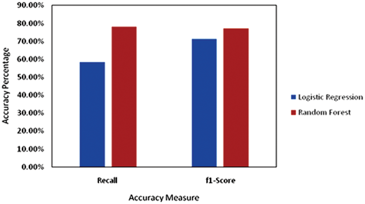
Figure 4: Graphical representation of accuracy measures for random forest

Model Accuracy Measures for Logistic regression, random forest, and gradient boosting can be observed in the following Fig. 5 and the Tab. 5. for the models Logistic regression, Random forest, and the Gradient boosting techniques.

Figure 5: Graphical representation of accuracy measures for different approaches

The graphical representation of the accuracy measures indicates that the Gradient Boosting Method can predict the ‘Loan Defaulters’ much better than Logistic Regression and Random Forest model.

6  Conclusion

This paper aimed to explore, analyze, and build a cpmparatve performances of different machine learning algorithm to correctly identify whether a person, given certain attributes, has a high probability to default on a loan. This type of model could be considered by Lending Club to identify certain financial traits of future borrowers that could have the potential to default and not pay back their loan by the designated time. The Random Forest Classifier provided the prediction with an accuracy of 80% while the Logistic regression method provided with an accuracy of 70%. Random Forest model appears to be a better option for such kind of data. One of the ensemble machine learning called Gradient Boosting algorithm shows the better result when comparing to other techniques and the accuracy has been shown as above 90%.

Sine gradient boosting model is performing with maximum efficiency among the three algorithms, it could further be considered for detecting and predicting loan fradulents. More avialibity of data may also help to improve the resuts. These alogorithms have been performing not up to that much satisfactory level, in further studies neural netwoks and deep learning would be incorporated.

In this paper traditional machine learning algorithms has been considered since the dataset having continuous values in tabular format. As per the literature survey, deep learning techniques are more effective on sequential data. So the future work will be carried out by comparing different conventional and deep learning algorithms on sequential as well as continuous data.

Funding Statement: The authors received no specific funding for this study.

Conflicts of Interest: The authors declare that they have no conflicts of interest to report regarding the present study.

References

1. 22-10-2021, 10:55AM. Available: https://spd.group/machine-learning/fraud-detection-with-machine-learning/. [Google Scholar]
2. 22-10-2021, 12:55PM. Available: https://spd.group/machine-learning/credit-card-fraud-detection-case-study/. [Google Scholar]
3. S. P. Maniraj, A. Saini, S. Ahmed and S. D. Sarkar, “Credit card fraud detection using machine learning and data science,” International Journal Of Engineering Research & Technology (IJERT), vol. 8, no. 9, pp. 110–115, 2019. [Google Scholar]
4. R. Pradheepan and G. Neamat, “Fraud detection using machine learning and deep learning,” in Int. Conf. on Computational Intelligence and Knowledge Economy (ICCIKE) in UAE, pp. 334–339, 2019. [Google Scholar]
5. E. W. T. Ngai, Y. Hu, Y. H. Wong, Y. Chen and X. Sun, “The application of data mining techniques in financial fraud detection: A classification framework and an academic review of literature,” Decision Support Sysemt, vol. 50, no. 3, pp. 559–569, 2011. [Google Scholar]
6. M. Ahmed, A. N. Mahmood and M. R. Islam, “A survey of anomaly detection techniques in financial domain,” Future Generation Computer System, vol. 55, no. 3, pp. 278–288, 2016. [Google Scholar]
7. M. Ahmed, N. Choudhury and S. Uddin, “Anomaly detection on big data in financial markets,” in Proc. of the 2017 IEEE/ACM Int. Conf. on Advances in Social Networks Analysis and Mining (ASONAM), Sydney, Australia, vol. 31, pp. 998–1001, 2017. [Google Scholar]
8. A. Abdallah, M. Aizaini and M. A. Zainal, “Fraud detection system: A survey,” Journal of Networking and Computational Application, vol. 68, no. 3, pp. 90–113, 2016. [Google Scholar]
9. K. Gai, M. Qiu and X. Sun, “A survey on FinTech,” Journal of Networking and Computational Application, vol. 103, no. 12, pp. 262–273, 2018. [Google Scholar]
10. N. F. Ryman-Tubb, P. J. Krause and W. Garn, “How artificial intelligence and machine learning research impacts payment card fraud detection: A survey and industry benchmark,” Engineering Applications of Artificial Intelligence, vol. 76, pp. 130–157, 2018. [Google Scholar]
11. J. West and M. Bhattacharya, “Intelligent financial fraud detection: A comprehensive review,” Computer Security, vol. 57, no. 6, pp. 47–66, 2016. [Google Scholar]
12. T. Pourhabibi, K. L. Ongb, B. H. Kama and Y. L. Boo, “Fraud detection: A systematic literature review of graph-based anomaly detection approaches,” Decision Support System, vol. 133, no. 4, pp. 58–72, 2020. [Google Scholar]
13. A. Singh, “Anomaly detection for temporal data using long short-term memory (LSTM),” IFAC-PapersOnLine, vol. 52, pp. 2408–2412, 2017. [Google Scholar]
14. W. Bao, J. Yue and Y. Rao, “A deep learning framework for financial time series using stacked autoencoders and long-short term memory,” A Deep Learning Framework for Financial Time Series, vol. 12, pp. 1–24, 2017. [Google Scholar]
15. K. K. Tripathi and M. A. Pavaskar, “Survey on credit card fraud detection methods,” International Journal of Emerging Technology and Advanced Engineering, vol. 2, no. 11, pp. 721–726, 2012. [Google Scholar]
16. J. R. Quinlen, “Introduction of decision trees,” Machine Learning, vol. 1, no. 1, pp. 81–106, 1986. [Google Scholar]
17. J. Han and M. Kamber, Data mining concepts and techniques. Elsevier, pp. 744, 2018. [Google Scholar]
18. S. B. Kotsiantis, “Supervised machine learning: A review of classification techniques,” Informatica, vol. 31, pp. 249–268, 2007. [Google Scholar]
19. G. J. Williams and Z. Huang, “Mining the knowledge mine: The hot spots methodology for mining large real world databases,” in Australian Joint Conference on Artificial Intelligence, Berlin, pp. 340–348, 1997. [Google Scholar]
20. F. M. Liou, Y. C. Tang and J. Y. Chen, “Detecting hospital fraud and claim abuse through diabetic outpatient services,” Health Care Management Science, vol. 11, no. 4, pp. 353–358, 2008. [Google Scholar]
21. H. Shin, H. Park, J. Lee and W. C. Jhee, “A scoring model to detect abusive billing patterns in health insurance claims,” Expert Systems with Applications, vol. 39, no. 8, pp. 7441–7450, 2012. [Google Scholar]
22. S. Maes, K. Tuyls, B. Vanschoenwinkel and B. Manderick, “Credit card fraud detection using bayesian and neural networks,” in Proc. of the First Int. NAISO Congress on Neuro Fuzzy Thechnologies, India, pp. 78–89, 2002. [Google Scholar]
23. M. Zareapoora and P. Shamsolmoali, “Application of credit card fraud detection: Based on bagging ensemble classifier,” International Conference on Intelligent Computing, Communication & Convergence (ICCC-2015Procedia Computer Science, vol. 48, no. 1, pp. 679–686, 2015. [Google Scholar]
24. K. Randhawa, K. L. Chu, S. Manjeevan, P. L. Chee and K. N. Asoke, “Credit card fraud detection using AdaBoost and majority voting,” IEEE Access, vol. 6, pp. 14277–14284, 2018. [Google Scholar]
25. A. Pumsirirat and L. Yan, “Credit card fraud detection using deep learning based on auto-encoder and restricted boltzmann machine,” International Journal of Advanced Computer Science and Applications(IJACSA), vol. 9, no. 1, pp. 18–25, 2018. [Google Scholar]
26. T. Sweers, “Autoencoding credit card fraud,” Ph.D .dissertation, Radboud University, Nijmegen, 2018. [Google Scholar]
27. Z. Chen, C. K. Yeo, B. S. Lee and C. T. Lau, “Autoencoder based network anomaly detection,” in Wireless Telecommunications Symposium, USA, pp. 1–5, 2018. [Google Scholar]
28. S. Magomedov, S. Pavelyev, I. Ivanova, A. Dobrotvorsky and M. Khrestina, “Anomaly detection with machine learning and graph databases in fraud management,” International Journal of Advanced Computer Science and Applications (IJACSA), vol. 9, no. 11, pp. 33–38, 2018. [Google Scholar]
29. D. Huang, D. Mu, L. Yang and X. Cai, “Codetect: Financial fraud detection with anomaly feature detection,” IEEE Access, vol. 6, pp. 19161–19174, 2018. [Google Scholar]
30. T. Amarasinghe, A. Aponso and N. Krishnarajah, “Critical analysis of machine learning based approaches for fraud detection in financial transactions,” in Proc. of the 2018 Int. Conf. on Machine Learning Technologies (ICMLT’18), Nanchang, China, 21-23, pp. 12–17, 2018. [Google Scholar]
31. J. Elith, J. R. Leathwick and T. Hastie, “A working guide to boosted regression trees,” Journal of Animal Ecology, vol. 77, no. 4, pp. 801–813, 2008. [Google Scholar]
32. T. K. Ho, “Random decision forests,” in Proc. of the 3rd Int. Conf. on Document Analysis and Recognition, Montreal, QC, 14-16, pp. 278–282, 1995. [Google Scholar]
33. T. K. Ho, “The random subspace method for constructing decision forests,” IEEE Transactions on Pattern Analysis and Machine Intelligence, vol. 20, no. 8, pp.832–844, 1998. [Google Scholar]
34. P. S. Madeh and E. D. Tamer, “Role of data analytics in infrastructure asset management: Overcoming data size and quality problems,” Journal of Transportation Engineering, Part B: Pavements, vol. 146, no. 2, pp. 41–53, 2020. [Google Scholar]
35. E. Kleinberg, “Stochastic discrimination,” Annals of Mathematics and Artificial Intelligence, vol. 1, no. 1–4, pp. 207–239, 1990. [Google Scholar]
36. E. Kleinberg, “An overtraining-resistant stochastic modeling method for pattern recognition,” Annals of Statistics, vol. 24, no. 6, pp. 2319–2349, 1996. [Google Scholar]
37. E. M. Kleinberg, “On the algorithmic implementation of stochastic discrimination,” IEEE Transactions on Pattern Analysis and Machine Intelligence, vol. 22, no. 5, pp. 473–490, 2000. [Google Scholar]
38. K. M. Suresh, “Credit card fraud detection using random forest algorithm,” in 3rd Int. Conf. on Computing and Communications Technologies (ICCCT), Inida, pp. 590–603, 2019. [Google Scholar]
39. L. Breiman, “Random forests,” Machine Learning, vol. 45, no. 1, pp. 5–32, 2001. [Google Scholar]
40. R. Hooman, T. Nam, B. Elham, H. Lydia and G. Ralph, “Artificial intelligence and machine learning in pathology: The present landscape of supervised methods,” Academic Pathology, vol. 6, pp. 546–558, 2018. [Google Scholar]
41. V. Dejan, “Credit card fraud detection-machine learning methods,” in 18th Int. Symp. INFOTEHJAHORINA (INFOTEH). IEEE, pp. 258–278, 2019. [Google Scholar]
42. D. Deepti, S. Patil and S. Kokate, “Detection of credit card fraud transactions using machine learning algorithms and neural networks: A comparative study,” in Fourth Int. Conf. on Computing Communication Control and Automation (ICCUBEA), India, pp. 390–409, 2018. [Google Scholar]
43. K. R. Seeja and M. Zareapoor, “FraudMiner: A novel credit card fraud detection model based on frequent itemset mining,” The Scientific World Journal, vol. 2014, no. 3, pp. 1–10, 2014. [Google Scholar]
44. M. B. Lakshmipriya and J. Jaiswal, “Credit card fraud detection using a combined approach of genetic algorithm and random forest,” International Journal of Trend in Scientific Research and Development (IJTSRD), vol. 4, no. 5, pp. 230–233, 2020. [Google Scholar]
45. K. R. Seeja and M. Zareapoo, “FraudMiner: A novel credit card fraud detection model based on frequent itemset mining,” pp. 1–10, The Scientific World Journal, 2014. [Google Scholar]
46. B. Gustavo, P. Ronaldo and C. M. Maria, “A study of the behavior of several methods for balancing machine learning training data,” ACM SIGKDD Explorations Newsletter, pp. 1–9, 2004. [Google Scholar]
47. M. W. Gary and P. Foster, “The effect of class distribution on classifier learning: An empirical study,” Rutgers University, vol. 5, pp. 459–467, 2001. [Google Scholar]
48. E. Andrew, J. Taeho and J. Nathalie, “A multiple resampling method for learning from imbalanced data sets,” Computational Intelligence, vol. 6, pp. 365–379, 2004. [Google Scholar]
49. V. C. Nitesh, “Data mining for imbalance datasets: An overview,” Data Mining and Knowledge Discovery Handbook, pp. 853–867, 2005. [Google Scholar]
50. J. Nathalie and S. Shaju, “The class imbalance problem: A systematic study,” Intelligent Data Analysis, vol. 1, pp. 258–269, 2002. [Google Scholar]
51. K. Miroslav and M. Stan, “Addressing the curse of imbalanced training sets: One-sided selection,” in Proc. of the Fourteenth Int. Conf. on Machine Learning, USA, pp. 179–186, 1997. [Google Scholar]
52. M. Inderjeet and I. Zhang, “KNN approach to unbalanced data distributions: A case study involving information extraction,” in Proc. of Workshop on Learning from Imbalanced Datasets, India, pp. 25–42, 2003. [Google Scholar]
53. A. Agresti, An introduction to categorical data analysis, 2nd ed., USA: A John Wiley & Sons, Inc., Publications, 2007. [Google Scholar]
54. C. Corinna and V. Vladimir, Support vectometwork and machnine learning, vol. 5, USA: Kluwer Academic Publishers, pp. 46–69, 1995. [Google Scholar]
55. D. C. Montgomery, E. A. Peck and G. Vining, Introduction to linear regression analysis, 3rd ed., USA: JohnWiley & Sons Inc, 2001. [Google Scholar]
56. E. Jane, “A working guide to boosted regression trees,” Journal of Animal Ecology, vol. 77, no. 4, pp. 802–813, 2008. [Google Scholar]
57. J. H. Friedman, “Greedy function approximation: A gradient boosting machine,” Journal of Machine Learning Research, vol. 1, pp. 90–96, 1999. [Google Scholar]
58. J. H. Friedman, “Multiple additive regression trees with application in epidemiology,” Journal of Statistics in Medicine, vol. 22, pp. 1365–1381, 2003. [Google Scholar]
59. E. Kleinberg, “On the algorithmic implementation of stochastic discrimination,” IEEE Transactions on PAMI, vol. 22, no. 5, pp. 473–490, 2000. [Google Scholar]
60. A. Tharwat, “Classification assessment methods,” Applied Computing and Informatics, vol. 1, pp. 2345– 2364, 2018. [Google Scholar]
61. T. Fawcett, “An introduction to ROC analysis,” Pattern Recognition Letters, vol. 27, no. 8, pp. 861–874, 2006. [Google Scholar]
62. D. M. W. Powers, “Evaluation: from precision, recall and f-measure to ROC, informedness, markedness & correlation,” Journal of Machine Learning Technologies, vol. 2, no. 1, pp. 37–63, 2011. [Google Scholar]
63. K. M. Ting, S. Claude and W. I. Geoffrey, Encyclopedia of machine learning, Boston: Springer, 2011. ISBN 978-0-387-30164-8. [Google Scholar]
64. D. Chicco and G. Jurman, “The advantages of the Matthews correlation coefficient (MCC) over F1 score and accuracy in binary classification evaluation,” BMC Genomics, vol. 21, no. 1, pp. 6.1–6.13, 2020. [Google Scholar]
65. D. Chicco, N. Toetsch and G. Jurman, “The Matthews correlation coefficient (MCC) is more reliable than balanced accuracy, bookmaker informedness, and markedness in two-class confusion matrix evaluation,” BioData Mining, vol. 14, no. 13, pp. 1–22, 2021. [Google Scholar]
66. S. Dhankhad, E. Mohammed and B. Far, “Supervised machine learning algorithms for credit card fraudulent transaction detection: A comparative study,” in 2018 IEEE Int. Conf. on Information Reuse and Integration (IRI), USA, pp. 118– 125, 2018. [Google Scholar]
Cite This Article
Copyright © 2023 The Author(s). Published by Tech Science Press.
This work is licensed under a Creative Commons Attribution 4.0 International License , which permits unrestricted use, distribution, and reproduction in any medium, provided the original work is properly cited.
Downloads
Citation Tools