DOI:10.32604/csse.2023.024943
| Computer Systems Science & Engineering DOI:10.32604/csse.2023.024943 | |
| Article |
Dynamic Ensemble Multivariate Time Series Forecasting Model for PM2.5
School of Computing, SASTRA University, Thanjavur, 613401, India
*Corresponding Author: Umamakeswari Arumugam. Email: aumaugna@gmail.com
Received: 05 November 2021; Accepted: 27 December 2021
Abstract: In forecasting real time environmental factors, large data is needed to analyse the pattern behind the data values. Air pollution is a major threat towards developing countries and it is proliferating every year. Many methods in time series prediction and deep learning models to estimate the severity of air pollution. Each independent variable contributing towards pollution is necessary to analyse the trend behind the air pollution in that particular locality. This approach selects multivariate time series and coalesce a real time updatable autoregressive model to forecast Particulate matter (PM) PM2.5. To perform experimental analysis the data from the Central Pollution Control Board (CPCB) is used. Prediction is carried out for Chennai with seven locations and estimated PM’s using the weighted ensemble method. Proposed method for air pollution prediction unveiled effective and moored performance in long term prediction. Dynamic budge with high weighted k-models are used simultaneously and devising an ensemble helps to achieve stable forecasting. Computational time of ensemble decreases with parallel processing in each sub model. Weighted ensemble model shows high performance in long term prediction when compared to the traditional time series models like Vector Auto-Regression (VAR), Autoregressive Integrated with Moving Average (ARIMA), Autoregressive Moving Average with Extended terms (ARMEX). Evaluation metrics like Root Mean Square Error (RMSE), Mean Absolute Error (MAE) and the time to achieve the time series are compared.
Keywords: Dynamic transfer; ensemble model; air pollution; time series analysis; multivariate analysis
Air pollution is a serious threat globally drawing above 8 million lives every year [1]. Recent study states the effects of air pollution on human health, increasing breathing diseases like asthma & bronchitis [2]. Developing countries like India are establishing the state of Particulate Matter with before and after covid-19 to built new strategies and environmental standards [3]. Among many air pollutants particulate matter plays an important role in estimating overall air quality. PM is fine solid particles drooping in air with size in micrometers. PM2.5 is analysed in this proposed method, PM’s is less in quantity in air when compared to the other major pollutants but its impact in human health is adverse. In developed countries like America, long term exposure to PM leads to many endemic problems [4]. European association of cardiovascular prevention and rehabilitation analyse the short term and long term mortality with exposure to PM [5]. It is necessary to forecast the adversity of the PM in India to build a new control measure and strategy to protect the environment.
Time series analysis helps in analysing the huge data to find the trend or seasonality behind it. Real time data analysis plays a vital role in creating human intelligence [6]. Various extended models such as VAR, Vector Auto-Regressive Moving Average (VARMA) have been extensively used in multivariate time series analysis for PM2.5 [7]. VAR incorporated in the error correction mechanism will explorate the long term prediction on multivariate time series data [8].
VARMA is widely used in finance and VAR is used for direct multi-step estimation in stationary and non-stationary processes [9]. Major drawback of VAR is the large number of parameters needed to estimate the model [10]. Recently fuzzy time series prediction models perform great in multivariate problems which handle multiple variables in a heuristic approach to increase the prediction result [11]. The combination of a fuzzy set with the neural network will provide better results in the high-voluminous time series data [12]. Some of the research work adores the fuzzy based time series to forecast the future with the historical data [13]. VARMA tends to be slow when we use unlabelled and realtime complicated data. Moreover the real-time application data is always tedious and large in nature which means the model takes more features which adds computational overhead [14]. Many models in literature deal with multivariate time series data, still forecasting a certain dependent variable has limitations.
The proposed method follows the combination of many time series models to make it more accurate in forecasting the pollution particles. Some of the methods involve correlating two or more forecasting techniques which yields a high end ensemble model with greater accuracy [15]. However, These ensemble methods for real-time forecasting has a limitation of increasing complexity when the number of models rises. Analogously forecasting algorithms with neural networks for multivariate time series data will take long training time and is computationally complex [16]. Recent works for real time prediction are now with ELMK (Extreme Learning Machine with Kernels) a novel approach combining multiple ELM (Extreme Learning Machine) which provide better accuracy with lesser order of magnitude [17]. It is evident that the real time forecasting on non-stationary time series provides improved performance by applying a fixed memory based prediction algorithm which eliminates the data from the past [18]. ARIMA models consider only one variable PM2.5 concentration without any external factors affecting it [19]. A new approach with Autoregressive moving average with exogenous input (ARMAX) is proposed to predict PM2.5 in account of weather parameters [20]. There are few online prediction models which help to predict the data instantly by applying versions of Newton and gradient descent algorithms, sometimes these algorithms can be given as a loss function to the ARMA model. Although many approaches are present in literature a new multivariate forecasting model is needed, the real-time univariate one is hard to collect many features. The Proposed state of art is given in Fig. 1.
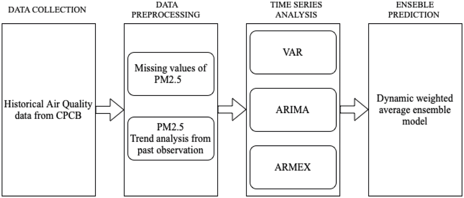
Figure 1: Ensemble model of multivariate time series forecasting of PM2.5
In this method multivariate sampled active transfer for stable real-time prediction is proposed with few lag towards the trend unlined with the datapoint. Time series analysis using a transfer model is formed from lagged regression where input variable X(t) affects the auto regression of the resultant variable ϒt. There are various methods to find the relationship between the input and the resultant variables. It is difficult to find the detriment of the lagged variable with respect to the uncertainty behind the input variables [21]. It is too empirical to find the lag between the input and output variable using cross correlation. Although some solutions are proposed with Monte Carlo based analysis to solve the lag between input and output variables [22]. An ensemble model incorporates various features from environment parameters from various locations and scales to the maximum benefit that we can get out of the model [23]. Fuzzy rules based granular time series along with support vector machine (SVM) is used to predict the concentration of PM2.5, still there is instability in predicting the concentration without considering the influencing pollutant [24].
Novel dynamic fetch approach selects various input variables from each lagged regression and creates a diverse active fetch model. Based on the selected input variables estimates the time series auto regressive analysis of output variables. It builds an initial ensemble model with instant training data and then forecast response variables by updating the basic model. Since there are many dynamic models that can create a diverse combination of variables with aggressive orders and different orders, the best model can be selected from the set of basic orders in an ensemble way. Weights of the base model updated consistently to make the model periodically reflect the unpredictable internal errors that are quite possible in air pollution prediction. Moreover the effects of memory are reduced, since the use of lagged information and immediate updating does not require much memory. It is blatant that the significant performance improvement in the proposed forecasting method by using ensemble active fetch of multivariate time series with high forecasting accuracy by correcting predict failures.
3 Multivariate Time Series Analysis
Classical TSA is used to analyse the trend or pattern behind the occurrence of the event. The Auto Regressive Integrated Moving Average (ARIMA) model is predominantly used to plot the X(t) with respect to time in the order p, d and q.
at is zero mean white noise at time t.
B is the shift backward operator.
ARMA is a sub-model of ARIMA where the difference d is assumed to be zero. ARMA works well for weak stationary stochastic processes with autoregressive moving averages. The difference order is zero, the polynomial of the moving average is invertible. The model may denote an infinite autoregressive moving average which is given in Eq. (2).
Delay b with noise nt the resultant variable would be Y(t)
The transfer functions with multiple input reflecting nonlinearity between the variables given in ARMA and the resultant variable, identifying these nonlinearity is trivial. The proposed dynamic transfer model integrates multiple algorithms to improve performance and make one ensemble forecasting model. The key component of the ensemble model is to have multiple random algorithms including diversity so numerically overfitting of the algorithm can be avoided. Bootstrap aggregating is overly adopted by choosing the subset of the training dataset, an Ensemble model can classify it from the basic algorithm denoted by f. It is usually associated with weights w, weight wi is often computed according to the performance of each f.
The proposed method encompasses two components one is transfer and another one is Dynamic ensemble model. Active fetching of models help to identify the common characters and the similarities between existing models. Whereas the integration of these models will be in dynamic nature to make reliable and accurate predictions for multivariate time series. Similar approach have been prosed with active transfer model [25].
4 Dynamic Transfer of Basic Time Series Model
Dynamic learning models use multivariate time series to come out with models that have accurate and stable performance. We take values initially with a fixed number of post observations and another one without a fixed number of post observations. Updating these models with respect to the weights associated to that model happens on an instant basis. The active fetch model combines dynamic lag in regression as the transfer function allows the model to adapt the parameter in instant fashion, considered it as a single time series with a multivariate response.
Order of p is the difference order d and the selector of the model is given by In x 1. Conditionally the d ≤ p model tries to determine the effect on the input signal to the response signal ϒt in a dynamic method. It captures several inputs using the selector I. Each model can have its effect of input variable X aligned with the gradual lag in its regression. ϒt modelled in infinite number of difference order with respect to Xt for a particular input signal which is exponentially festering the model, can be dependent variable ϒt is given in Eq. (5).
The Active fetch model explores the similarity between the input variable with Auto Regressive Moving Average External terms (ARMEX). ARMEX is an exemplary model which takes the difference between the two basic models. The proposed method considers the input variable to be stochastic to the dependent variable and it will be the response of the second basic model which is selected by selectors I. This approach enables the model to generate several meaningful insights and later aggregate these models to frame an ensemble one.
Ensemble model has certain computational challenges which try to figure out the relationship between the input signal and the resultant variable ϒt at all points of time T. Stochastic processes try to explain the ϒt using the input variable at a certain fixed time using their predict failure to check the model to be enclosed in ensemble approach with particular difference order d. Further aim is to reduce the lag between the input variable and output variable with respect to the pattern aligned originally behind it. Several strategies such as empirical analysis of autocorrelation, numerical search of the lowest standard deviation and theoretical verification of stationarity is adopted. Target model is to fix the value of p, d and I to be in optimal manner and it is nontrivial, but challenging part is the empirical analysis of autocorrelation numerical search among the lowest standard deviation and its theoretical verification, to overcome this challenge that the difference of order is choosen from 1 to D. Different strategy can also be applicable for the value of π from which I can derive models to make the ensemble model by estimating least lack regression.
The proposed approach represents the prediction signal by available least lag models after the current time T predicting the T++. This procedure is commonly observed when we take random input from an axillary model [26]. We have N + 1 step of prediction using the N observation until the time T.
5 Aggregating Models to Derive Ensemble Forecasting Model with Dynamic Transfer
For accurate and reliable instant prediction using multivariate time series an ensemble model helps to create numerous active transfer models from the basic lag between the input and output. The selection of the model to be made in a way that the fixed amount of past data or the records of least squares to become in a consecutive manner so that the model can be built using the trained observation. With this top k models to make the input variable with minimum prediction error aligned to the output variable. Generate a prediction model from the repeated training to reduce the d which helps to stop the huge predict failures.
The ensemble model needs h-step prediction models to test before reaching the optimised active transfer, Particularly it considers the model with the least auto regressive order of p and the difference order ranges from 1 to D. It generates large number of models {Y(t)}ⁿ with pⁿ, qⁿ and Iⁿ as q should not greater than n, this makes the model computationally feasible. Ensemble model apply a weighting technique based on the prediction error, As {Y(t)}ⁿ is the model with weight wⁿ, while training the model it is normalised and given by Eq. (6).
In particular, we need to build the appropriate model with respect to the past observation. The parameter G is the number of past performance observations. Assuming the weight is inversely proportional to the sum of the squared error, larger wⁿ makes the model better. We choose top K models to make the ensemble model as given in Eq. (7).
The prediction of the each input variable Xn with respective autoregressive order from 1 to Pⁿ, the difference order from 1 to Dⁿ, which yields K feasible model. The h-step prediction is observed based on that instant time T will give the coefficients, We have two options in updating the ensemble model one with fixing a number past observation and another one with recursive least squares to update the coefficients. With one fixed number of past observation, models help to calculate the coefficient and store them in the instant data with its fixed memory size. Next one update the recursive least square by storing them in the memory update the performance weight wⁿ to get the most recent best k-models.
6 Experiment Results and Discussion
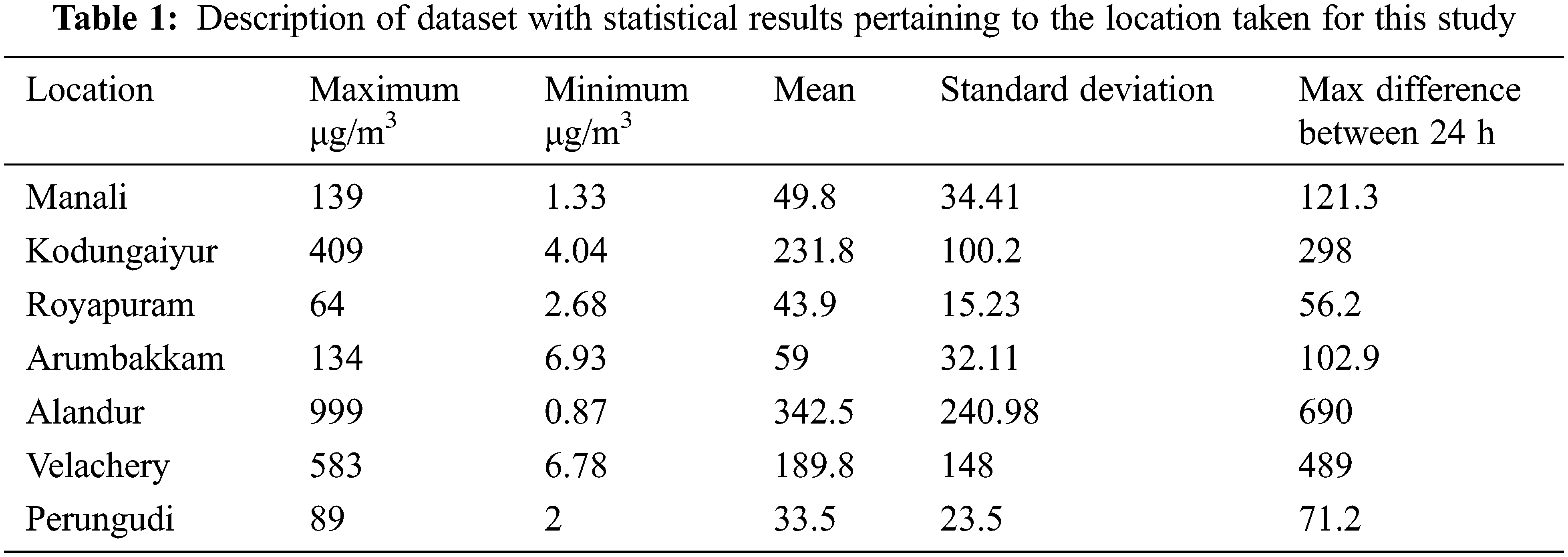
For validating the Ensemble model, Chennai is taken. Chennai is a multiphase city with a large number of industries and it has a population of 7 Million. Manali, Kodungaiyur, Royapuram, Arumbakkam, Alandur, Velachery and Perungudi are the seven locations taken with a 24 hr sample of PM2.5 from CPCB. Data from 2015 to 2018 analysed and used for training, 2019 its is used for testing and 2020 is used for validating the model. Root Mean Square Error (RSME) and Mean Absolute Error (MAE) values are evaluated for different time bounds. To contemplate the performance evaluation of the long term forecasting five sets of timestamp t + 1, t + 2, t + 4, t + 6, t + 12 were taken. Three traditional models were taken and compared with the proposed system VAR, ARIMA, ARMEX. For ARIMA model P = 8, difference order d = 4, P’ = 6 with K = 50 and the maximum models that can be built is limited to 100. I selectors may select 8 best base models to cumulate it into an ensemble one.
The time takes to compute the models and the RMSE is analysed and plotted for the five timestamps. The seven loactions around chennai is tabulated in Tab. 1 along with its data spread. In python statsmodel package VAR is extracted and found that t + 1 time bound VAR performed better.
Traditional ARIMA model is usually adopted to achieve good forecasting in random input. Whereas the Seasonal ARIMA (SARIMA) is used in some locations where the yearly pollution has certain seasonality behind. This seasonality is verified by the dicky-fuller test. Ensemble model built eight independent time series x1, x2, x3,…x8 form an ARIMA model with Autoregressive coefficients ranges between −1 to 1. A preset range is selected within the predictable difference order D with its linear combination with respect to the input variable x(t). We have samples of 6000 to 8000 numbers for training and the ensemble method predicts the concentration of PM2.5 & PM10. The missing values of the data were replaced by the local mean with respect to ±6 days. Each reference model is taken with a h-step of training so the error in lag prediction may be eradicated. Prediction is carried out for the next 12 days with different timestamps and it is clear that the ensemble model provides better performance for long-term time series forecasting t + 6, t + 12 whereas even the short-term forecasting t + 1, t + 3 ensemble model with varying weights provide stable forecasting performance for longer duration. ARIMA provide s the lowest error in short term forecasting. The weighted Ensemble model provides lower error rate for long term prediction.
It is evident that the deviation of the predicted value and the actual value is really close in forecasting PM2.5 using the weighted ensemble model. A model in forecasting is evaluated with reasonable time and efficiency by its accuracy with lag of 1 or 2 s the proposed ensemble model stable and deterministic performance when compared to VAR, ARIMA & ARMEX. The consistency of the ensemble approach increases if the prediction is long term. RSME is twice lower than the traditional methods which proves the strength of the dynamic ensemble model. It is clear that the prediction goes with least error when the predicted forecast is long term in case of the ensemble model. Most of the cases the Ensemble method gives the least RMSE. The MAE value of the proposed method is compared with other models tabulated in Tab. 2. The RMSE values for the proposed method along with traditional methods for all the seven locations is plotted in Fig. 2. From MAE and RMSE values, the proposed Ensemble method provides least value when compared to other methods. Observation period given with this study is three years and testing the model with 2019 prediction takes place for the year 2020. The proposed ensemble model is capable of understanding the temporal dependency of their historical value. The time-series model is trained for 24 hr data to get the next timestamp target t++. In general the production hour increases there is a drop in efficiency of the forecasting. But in controvert the proposed model gives better prediction accuracy in higher timestamped targets.
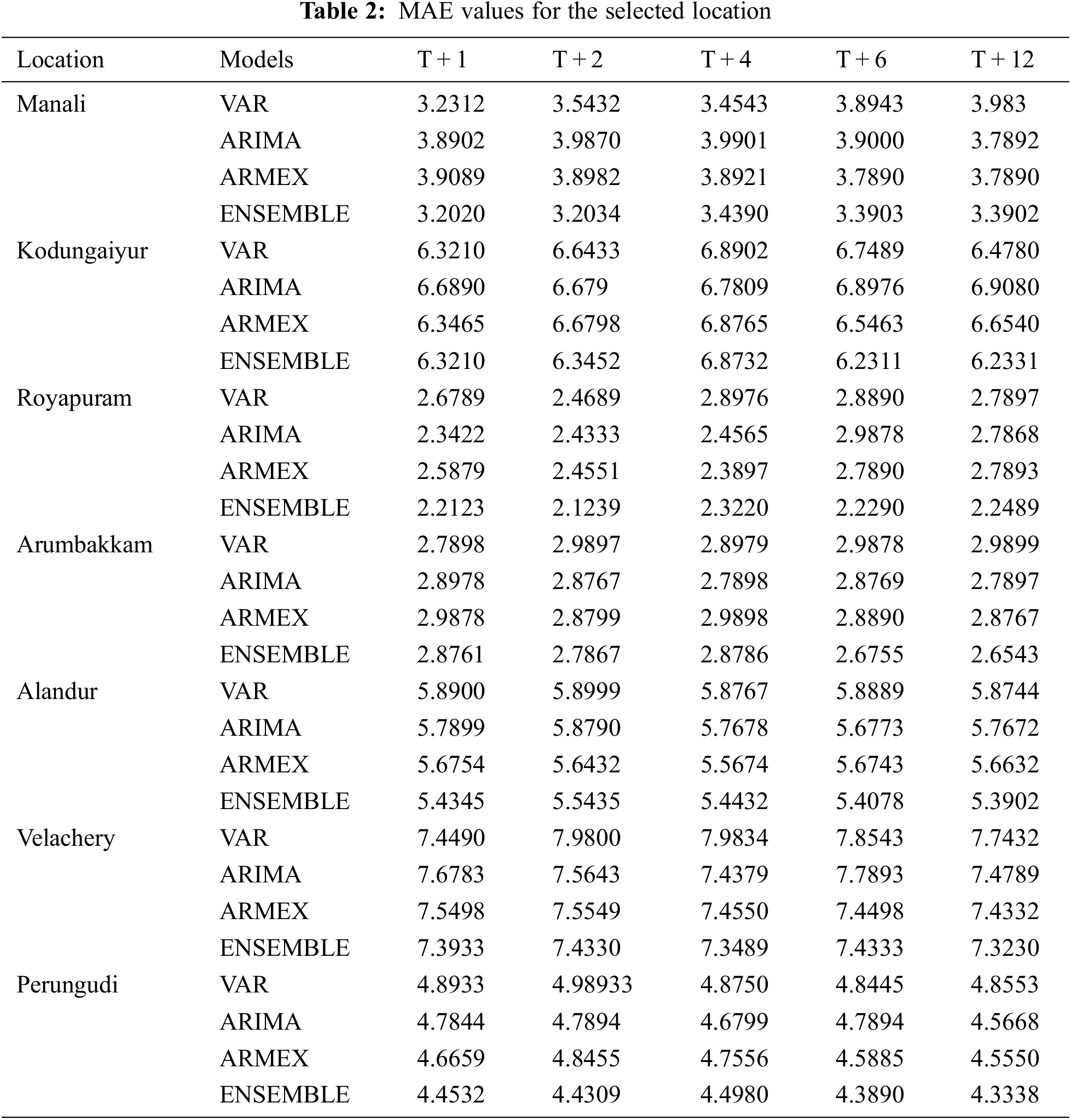
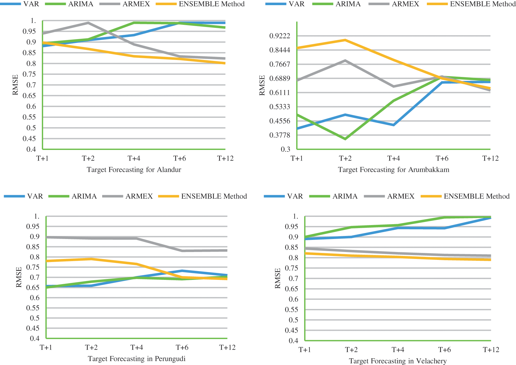
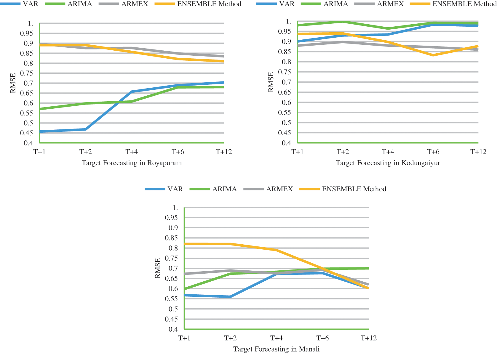
Figure 2: RMSE comparison of ensemble model with other models for the selected locations
Air pollution prediction is usually done with deep learning models with LSTM and Neural Networks, Since gated encoders have the memory to have the past historical values. Time series help to analyse the trend and pattern behind the pollutants to a particular geographical location. These trend predictions help in getting the nature of the increase in pollution in that particular locality. Transfer models in dynamic nature including ARIMA and some classical forecasting methods give consistent predictions for the long term. Proposed method makes ensemble models with these base TSA models instantaneously. The computation time decreases with several models of VAR, ARMEX are accounted, Parallel processing is used to find the top k basic accurate model then it leads to the ensemble approach. The weighted ensemble approach is accurate for long term prediction t + 6 and t + 12 with its prominent weighting used to build. In real time Atmospheric pollution is interrelated stochastic and multivariate in nature, this requires multivariate time series analysis and also active fetch of models in ensemble way. Pollutant PM2.5 is forecasted for the next 12 days with respect to the weighted ensemble model that is prevalent in all the seven locations taken for this study. The future work is to tune the model with some other external atmospheric factors.
Acknowledgement: We appreciate the air quality data provided by the Central Pollution Control Board, Ministry of Environment, India.
Funding Statement: The authors received no specific funding for this study.
Conflicts of Interest: The authors declare that they have no conflicts of interest to report regarding the present study.
1. J. Orach, C. F. Rider and C. Carlsten, “Concentration-dependent health effects of air pollution in controlled human exposures,” Environment International, vol. 150, pp. 106424, 2021. [Google Scholar]
2. P. E. Pfeffer, I. S. Mudway and J. Grigg, “Air pollution and asthma: Mechanisms of harm and considerations for clinical interventions,” Chest, vol. 159, no. 4, pp. 1346–1355, 2021. [Google Scholar]
3. U. C. Kulshrestha, “`New normal’ of COVID-19: Need of new environmental standards,” Current World Environment, vol. 15, no. 2, pp. 151–153, 2020. [Google Scholar]
4. S. Rajagopalan, M. Brauer, A. Bharnagar, D. L. Bhatt, J. R. Brook et al., “Personal-level protective actions against particulate matter air pollution exposure: A scientific statement from the American heart association,” Circulation, vol. 142, no. 23, pp. e411–e431, 2020. [Google Scholar]
5. S. Abohashem, M. T. Osborne, T. Dar, N. Naddaf, T. Abbasi et al., “A leucopoietic-arterial axis underlying the link between ambient air pollution and cardiovascular disease in humans,” European Heart Journal, vol. 42, no. 7, pp. 761–772, 2021. [Google Scholar]
6. P. K. Goswami and A. Sharma, “Realtime analysis and visualization of data for instant decisions: A futuristic requirement of the digital world,” Materials Today: Proceedings, vol. 2, no. 193, pp. 193, 2021. [Google Scholar]
7. P. J. García Nieto, F. Sánchez Lasheras, E. García-Gonzalo and F. J. de Cos Juez, “PM10 concentration forecasting in the metropolitan area of Oviedo (Northern Spain) using models based on SVM, MLP, VARMA and ARIMA: A case study,” Science of the Total Environment, vol. 621, pp. 753–761, 2018. [Google Scholar]
8. M. Rosenblatt and M. N. Quenouille, “The analysis of multiple time series,” Econometrica, vol. 27, no. 3, pp. 509, 1959. [Google Scholar]
9. G. Chevillon and D. F. Hendry, “Non-parametric direct multi-step estimation for forecasting economic processes,” International Journal of Forecasting, vol. 21, no. 2, pp. 201–218, 2004. [Google Scholar]
10. C. Gong, P. Tang and Y. Wang, “Measuring the network connectedness of global stock markets,” Physica A: Statistical Mechanics and its Applications, vol. 535, pp. 122351, 2019. [Google Scholar]
11. K. Huang, Huarng, T. H. Kuang Yu and Y. W. Hsu, “A multivariate heuristic model for fuzzy time-series forecasting,” IEEE Transactions on Systems, Man, and Cybernetics, Part B (Cybernetics), vol. 37, no. 4, pp. 836–846, 2007. [Google Scholar]
12. E. Egrioglu, C. H. Aladag, U. Yolcu, V. R. Uslu and M. A. Basaran, “A new approach based on artificial neural networks for high order multivariate fuzzy time series,” Expert Systems with Applications, vol. 36, no. 7, pp. 10589–10594, 2009. [Google Scholar]
13. C. H. Cheng and C. H. Chen, “Fuzzy time series model based on weighted association rule for financial market forecasting,” Expert Systems, vol. 35, no. 4, pp. e12271, 2018. [Google Scholar]
14. E. Isufi, A. Loukas, N. Perraudin and G. Leus, “Forecasting time series with VARMA recursions on graphs,” IEEE Transactions on Signal Processing, vol. 67, no. 18, pp. 4870–4885, 2019. [Google Scholar]
15. R. Adhikari and R. K. Agrawal, “A novel weighted ensemble technique for time series forecasting,” in Advances in Knowledge Discovery and Data Mining, Pacific-Asia Conf. on Knowledge Discovery and Data Mining, Berlin, Heidelberg: Springer, vol. 7301, pp. 38–49, 2012. [Google Scholar]
16. A. Borovykh, C. W. Oosterlee and S. M. Bohté, “Generalization in fully-connected neural networks for time series forecasting,” Journal of Computational Science, vol. 36, pp. 101020, 2019. [Google Scholar]
17. X. Wang and M. Han, “Online sequential extreme learning machine with kernels for nonstationary time series prediction,” Neurocomputing, vol. 145, pp. 90–97, 2014. [Google Scholar]
18. O. Anava, E. Hazan, S. Mannor and O. Shamir, “Online learning for time series prediction,” in Conf. on Learning Theory, Princeton, NJ, USA, pp. 172–184, 2013. [Google Scholar]
19. P. Wang, H. Zhang, Z. Qin and G. Zhang, “A novel hybrid-garch model based on ARIMA and SVM for PM 2.5 concentrations forecasting,” Atmospheric Pollution Research, vol. 8, no. 5, pp. 850–860, 2017. [Google Scholar]
20. Y. Hui, Y. Jing, Y. Xuyao, Z. Lixin and C. Wenliand, “Tracking prediction model for PM2.5 hourly concentration based on ARMAX,” Journal of Tianjin University (Science and Technology), vol. 50, no. 1, pp. 105–111, 2017. [Google Scholar]
21. R. M. Kuiper and O. Ryan, “Meta-analysis of lagged regression models: A continuous-time approach,” Structural Equation Modeling: A Multidisciplinary Journal, vol. 27, no. 3, pp. 1–18, 2019. [Google Scholar]
22. L. Keele, “Dynamic models for dynamic theories: The ins and outs of lagged dependent variables,” Political Analysis, vol. 14, no. 2, pp. 186–205, 2005. [Google Scholar]
23. P. S. Adhvaryu, “A review on diverse ensemble methods for classification,” IOSR Journal of Computer Engineering, vol. 1, no. 4, pp. 27–32, 2012. [Google Scholar]
24. S. Chen, J. Wang and H. Zhang, “A hybrid PSO-SVM model based on clustering algorithm for short-term atmospheric pollutant concentration forecasting,” Technological Forecasting and Social Change, vol. 146, pp. 41–54, 2019. [Google Scholar]
25. M. Oliveira and L. Torgo, “Ensembles for time series forecasting,” in Asian Conf. on Machine Learning, Hong kong, pp. 360–370, 2015. [Google Scholar]
26. K. M. Murphy and R. H. Topel, “Estimation and inference in two-step econometric models,” Journal of Business & Economic Statistics, vol. 3, no. 4, pp. 370, 1985. [Google Scholar]
 | This work is licensed under a Creative Commons Attribution 4.0 International License, which permits unrestricted use, distribution, and reproduction in any medium, provided the original work is properly cited. |