Computer Systems Science & Engineering DOI:10.32604/csse.2023.024277
Article

An Imbalanced Dataset and Class Overlapping Classification Model for Big Data

Mini Prince1,* and P. M. Joe Prathap2

1Department of Information Technology, St. Peter’s College of Engineering and Technology, Chennai, 600054, Tamilnadu, India
2Department of Information Technology, R.M.D Engineering College, Chennai, 601206, Tamilnadu, India
*Corresponding Author: Mini Prince. Email: miniprince171@gmail.com
Received: 12 October 2021; Accepted: 17 January 2022

Abstract: Most modern technologies, such as social media, smart cities, and the internet of things (IoT), rely on big data. When big data is used in the real-world applications, two data challenges such as class overlap and class imbalance arises. When dealing with large datasets, most traditional classifiers are stuck in the local optimum problem. As a result, it’s necessary to look into new methods for dealing with large data collections. Several solutions have been proposed for overcoming this issue. The rapid growth of the available data threatens to limit the usefulness of many traditional methods. Methods such as oversampling and undersampling have shown great promises in addressing the issues of class imbalance. Among all of these techniques, Synthetic Minority Oversampling TechniquE (SMOTE) has produced the best results by generating synthetic samples for the minority class in creating a balanced dataset. The issue is that their practical applicability is restricted to problems involving tens of thousands or lower instances of each. In this paper, we have proposed a parallel mode method using SMOTE and MapReduce strategy, this distributes the operation of the algorithm among a group of computational nodes for addressing the aforementioned problem. Our proposed solution has been divided into three stages. The first stage involves the process of splitting the data into different blocks using a mapping function, followed by a pre-processing step for each mapping block that employs a hybrid SMOTE algorithm for solving the class imbalanced problem. On each map block, a decision tree model would be constructed. Finally, the decision tree blocks would be combined for creating a classification model. We have used numerous datasets with up to 4 million instances in our experiments for testing the proposed scheme’s capabilities. As a result, the Hybrid SMOTE appears to have good scalability within the framework proposed, and it also cuts down the processing time.

Keywords: Imbalanced dataset; class overlapping; SMOTE; MapReduce; parallel programming; oversampling

1  Introduction

Due to the tremendous expansion of a large number of sensor networks, the internet of things, and smart gadgets, the world is being carried away by an immense quantity of data created from a wide variety of resources including social networks, sensor network data, video streaming sites, and internet marketing. Extraction of information from certain massive data sources is a significant challenge for a majority of conventional machine learning techniques. Due to the difficulties and complexities inherent in processing, interpreting, and extracting relevant information from such massive amounts of data, a new concept dubbed “big data” has been developed. In the data mining world, big data is a significant research topic as it is required in so many fields, including bioinformatics, marketing, medicine, and so on. In other words, it might be described as the data that necessitates the use of novel procedures, algorithms, and analyses for uncovering the hidden knowledge. It may be difficult for the standard data mining techniques to properly analyze such a large volume of data in an acceptable period. This problem may be solved with the help of new cloud platforms and parallelization technologies [1].

When the data volume is large, the traditional data mining algorithm [2] may not be suitable. Big data is said to be defined by characteristics such as volume, variety, velocity, and veracity. In the big data community, these are known as the “four V’s.” These four qualities have been used for categorizing these diverse issues. The massive volume that represents the enormous amount of collected data appears to be the most essential aspect among the 4 V characteristics of big data, as well as the largest problem [3]. While there are various and different sources of big data being created these days, the Internet of things, online social networks, and biological data are regarded as the three primary sources of big data. Apart from that, the quantity of data created and stored increases dramatically as the cities are getting smarter with more number of sensors. Every day, sensors and actuators worn by the patients create, store, and process millions of patient records in the e-health bioinformatics sector [4]. When it comes to big data, another difficulty is the enormous amount of variety it contains. As this big data is drawn from a wide variety of sources it might comprise of data of various file formats such as, images, videos, text, and so on. Another problem with big data is its enormous velocity that corresponds to the speed at which it is generated. As a result of the same, efficient and effective real-time processing methods are required [5]. Due to the shortage of resources and inadequate analytic tools, not all big data available today can be handled correctly for the extraction of essential information. As a result, a large amount of massive data that has to be handled would be put off, ignored, or erased. Thus, a large portion of the networking resources such as power, storage, and bandwidth are being diminished.

One of the major issues confronting big data is the problem of class imbalances and class overlaps. These two issues have made the construction of effective classifiers in data mining process tedious and hence results in severe performance losses. If the distribution of the dataset’s majority and minority classes appears to be unequal, then the class imbalance type of issues may arise. Class imbalances may range from modest to severe in the real-world type of settings (high or extreme). There are two classes in a dataset: majority and minority. The minority class possesses a small representation in the dataset, hence it’s frequently regarded as the most interesting one. Class imbalance can be expected while using the real-world datasets. A classifier may provide a high overall accuracy if the majority class has a severe class imbalance, as the model is likely to predict that most cases belong to the majority class. Such a model isn’t realistic as the data scientists care more about the forecast performance of the target class (i.e., the minority class) [6]. Many solutions have been developed for addressing these problems such as the under-sampling, oversampling, cluster-based sampling, and the Synthetic Minority oversampling techniques. Even though these methods have been found to offer better results in overcoming the class imbalance problems it has limited to problems with no more than the limited amount of data in the practical applications. When the data becomes huge in the real world problems these techniques appear to be inefficient. Under-sampling, oversampling, cluster-based sampling, and Synthetic Minority oversampling approaches are some of the ways that have been proposed for addressing these issues.

When there is an imbalance in a population, random under-sampling is a straightforward solution (or imbalanced data). When there is a lot of training data, this is a frequent approach. Random under-sampling removes the samples from the majority class at random until the classes are evenly distributed across the remaining dataset. As straightforward as this technique may be, there are several known downsides. Samples from the majority class are being randomly removed, and this may lose some relevant information from the dataset needed to train the model. As a result, a model trained on this smaller training dataset may not generalize adequately to the larger test dataset. Random over-sampling is very similar to random under-sampling in terms of the technique. The samples of the majority class would not be reduced this time; instead, the samples of the minority class would be increased. When the training data is limited and under-sampling isn’t a possibility, this method would be preferred. When using this method, no information is lost, and it has been found to outperform under sampling on the test data. The disadvantage of this method is that the replicating members of a minority class may lead to overfitting.

In order to avoid overfitting, SMOTE (synthetic minority oversampling technique) oversamples the minority class (unlike random over-sampling that has overfitting problems). SMOTE provides fresh synthetic data points based on a subset of the minority class. To make room for the minority class in the original training dataset, these new data points are generated. The SMOTE method avoids the problem of overfitting induced by random over-sampling by not reproducing the cases. Second, there is no information loss as the data points are never eliminated from the dataset. Synthetic instance creation has been illustrated in Fig. 1.

Figure 1: Synthetic instance creation in SMOTE

Even though these strategies have provided a better solution to the problem of class imbalance, their practical use has been confined to the problems with a small amount of data. When the amount of data in a real-world problem grows large, these strategies do not perform as well. The MapReduce framework is one of the appropriate options for dealing with enormous data sets since it is both easy and reliable. The MapReduce algorithm is a type of parallel programming. As opposed to the other parallelization systems such as the Message Passing Interface, its use for data mining has been highly encouraged dueto its fault-tolerant approach (preferred for time-consuming activities) [7]. MapReduce is a programming technique and software framework meant for handling large volumes of data. The Map and Reduce parts of the MapReduce software work together shown in Fig. 2. The Map and Reduce jobs have been found to deal with the dividing and mapping tasks of the data respectively.

Figure 2: MapReduce framework

It stands out for its high degree of transparency for the programmers, making it possible to easily and comfortably parallelize the applications. The MapReduce algorithm consists of two-phase namely the map and the reduce. Initially, it maps the data, and then it reduces it. Each phase incorporates key-value (A, V) pairs as input and output. Each stage incorporates key-value (A, V) pairs as input and output. (A, V) pairs have been used for storing an array of intermediate values. These pairs are created during the map phase and are used for collecting the data from the disc. This process would then be followed by a list-based shuffle of the values associated with that of the intermediate key. The reducing stage would consider the resultant list and would apply some operations to it before returning the system’s final response. Fig. 1 depicts the framework’s flowchart. The mapping and reducing procedures would be carried out at the same time. Every map function starts by running by itself. When it comes to reducing operations, they must wait until the end of the map has passed before continuing. Next, each of the individual keys would be processed in a separate and parallel manner. A MapReduce job’s inputs and outputs would be stored in a distributed file system that can be accessed by any of the computers in the cluster.

The MapReduce framework processes the data by reducing a large set of datasets into a small set of subsets through the use of the map and reduce functions. Reference [8] demonstrates the use of the map reduces framework for task scheduling in a cloud computing environment for the purpose of reducing the computation overhead. By taking advantage of the map-reduce parallel paradigm and by addressing the issue of an unbalanced dataset and class overlapping problem, we have proposed a hybrid under-sampling method. The main contribution of this paper comprises of three-stages as stated below:

1.    The first stage constitutes to the splitting of data into different blocks using a mapping function.

2.    In the second stage, a pre-processing technique would be applied to the individual mapping blocks that uses a hybrid SMOTE algorithm for solving the class imbalanced problem.

3.    Finally, a decision tree model would be built on the individual map blocks and these decision tree blocks would then be aggregated for creating a classification model.

The remainder of the paper has been structured as follows. Section II would provide a review of the related works in big data handling imbalanced data sets. Section III would provide a brief explanation of the proposed method. Section IV comprises of the experimental analysis, and Section V would conclude the entire work.

2  Related Work

Because of the rise of BigData, the issue of class imbalance has been accelerated even further. Unless specific methods are used, traditional classifiers cannot handle the imbalance between the classes. Traditional methods for addressing this problem includes the procedure of rebalancing the training set at the data level [9], tailoring algorithmic solutions to minority classes [10], and using cost-sensitive solutions that considers the various types of costs into account based on the distribution of classes [11]. Ensemble learning can be achieved by modifying or adapting the ensemble learning algorithm [12] itself, as well as one or more methods described previously, namely at the data level or through the algorithmic approaches that uses cost-sensitive learning as their foundation [13]. For an imbalanced dataset, many typical learning and classification algorithms tend to correctly classify the majority class while incorrectly classifying the minority class [14]. This discrepancy in the accuracy rate causes the classifier to underperform while diagnosing the samples from the minority groups. As a result, classifying an unbalanced dataset is a difficult task. It’s more critical to identify minority class samples in some contexts than that of the majority class samples [15].

Data-level solutions appear to be the most adaptable type of solutions as they can be used with any type of classifiers. The various types of approaches that can be used here would include the oversampling, the undersamplingand the hybrid type of techniques. The simplest type of technique is the random under-sampling technique that gradually eliminates the instances from the majority class. On the other hand, this may indicate that the critical examples from the training data have been overlooked. On the other hand, random oversampling precisely copies the minority instances. The disadvantage of this strategy is that it raises the likelihood of overfitting by strengthening all minority clusters regardless of their actual contribution to the problem. By eliminating the samples from the majority class through under-sampling and increasing the samples from the minority class through over-sampling, data re-sampling can assist in balancing the distribution of data classes. As a result, over-sampling may result in the border or noisy data, higher processing time, and inefficient over-fitting.

In the oversampling processing of the sample sets, the SMOTE algorithm has demonstrated good performance. In order to build fresh training sets, the algorithm can combine the newly created sample points from the minority class with that of the original dataset. This method can produce new sample points for the minority classes based on a rule [16]. Using this method, new minority class samples can be selected, copied, and synthesized, this helps in mitigating the over-learning problems associated with that of the random over-sampling. This method, however, does not account for the samples created by the new minority classes. In the oversampling process, minorities play a variety of sample roles, with those on the border playing a larger role than those in the center, and vice versa. Taking samples at the edge of the minority class can increase the classification decision surface recognition rates, whereas taking the samples in the minority class center can reduce the dataset unbalance rates. An improved SMOTE algorithm [17] has been proposed demonstrating that SMOTE is vulnerable to class overlapping. Han [18] proposed the borderline-SMOTE approach. If there are more majority class samples nearby than the minority class samples, it covers the samples located on the border of the minority class samples. Afterwards, the boundary samples of the minority classes would then be over-sampled, resulting in relevant area interpolation. After adding fresh minority class samples Chawla [19] developed the SMOTE Boost method for improving the prediction performance of the minority classes by combining the lifting and the sampling procedures. By detecting the samples that are difficult to distinguish between the majority and the minority groups, DataBoost-IM [20] can essentially solve the problem. Once the synthesizing samples are created, they would be employed in the process of creating new ones. At last, the new dataset would possess an equitable distribution of the category weights.

A popular strategy for re-sampling is to under-sample for saving the time by lowering the number of training sets and the total training length. Several under-sampling algorithms have been devised, including the condensed nearest-neighbor rule, the neighborhood-cleaning rule, one-sided selection, and the Tomek connection. They apply rules, procedures, and data overlapping for identifying and eliminating the majority of class samples that contribute nothing to the categorization process. Finally, they would employ the classifier’s test set that is composed of extremely small and safe class samples. To reduce the total population size of those members of the majority class, random samples from the bigger majority class would be lowered. As a result, useful information about the majority class would be easily lost, and the samples may exclude potentially useful and critical information.

It is better to reduce the entire cost of misclassification rather than just the error rates when using the cost-sensitive learning algorithm and sample method [21]. As they’re worried about the cost of misclassification, they tend to offer the minority group a very high misclassification cost. In this method, the classifier may improve the classification accuracy rate for the minority classes, hence resolving the issue of imbalanced data processing [22]. By altering the classification algorithm for making it more cost-sensitive, the cost-sensitive learning technique can produce suboptimal results. Although the standard active learning strategy can be used for tackling the unbalanced training data, it occasionally suffers from a class overlapping problem. When it comes to resolving the issue of class imbalance, traditional sampling procedures have proven to be extremely effective. While this is theoretically possible, the practical application has been limited to issues where there are just several hundred thousand examples. Most of the classical classifiers have been caught in the local optimum problem while dealing with enormous datasets, and they have been found to consume longer time durations for running their operations. Followed by this, numerous data mining techniques [23] have been widely utilized in the imbalanced datasets for converting them to balanced datasets using different sampling approaches like the random under sampling, the random oversampling and the SMOTE, MSMOTE, borderline SMOTE, etc [24–28]. The most common disadvantage in all these techniques isthatit works well only in a limited volume of data. If the volume of the data exceeds some specified set of limits, the performance of the algorithm degrades the overall efficiency in all aspects.

We have proposed a hybrid SMOTE Algorithm using the MapReduce framework for overcoming both the class overlapping and the class imbalanced data set and for reducing the the running time as well. Our proposed method has been divided into four stages. The first stage involves in the task of splitting the data into different blocks using a mapping function, followed by the application of a pre-processing procedure into the individual mapping blocks that utilizesa hybrid SMOTE algorithm for solving the class imbalanced problem. A decision tree model would be built on the individual map blocks. Finally, the decision tree blocks would be aggregated for forming a classification model.

3  Proposed Work

In this section, we would discuss in detail about the proposed work. Our aim is to build a hybrid SMOTE Algorithm using the MapReduce framework for overcoming both the class overlapping and the class imbalanced data set. In this contribution, we have used the advantage of a parallel programming in the MapReduce framework for reducing the long time run when datasets are large. To leverage the MapReduce framework, we have executed numerous Hybrid SMOTE processes shown in Fig. 4, on various chunks of the training data, resulting in as many reduced sets as mappers in the pipeline. Each of these datasets have been used for generating a decision tree model that would then be integrated during the reduction step for forming a classifier ensemble. Using the MapReduce-based SMOTE, we have constructed a decision tree-based ensemble for categorizing the imbalanced huge data. Fig. 3 illustrates our proposed model. To completely integrate the Hybrid SMOTE into the MapReduce model, two fundamental operations have been built, namely, the map and the reduce.

Figure 3: Proposed method

Figure 4: Hybrid SMOTE algorithm flow chart

3.1 Mapping Phase

In the MapReduce phase, the training dataset has been divided into several subsets, each of which would comprise of a different computing node. In each of these nodes, the hybrid SMOTE has been used, which may not be possible when considering the entire data set. The map consists of three parts as follows:

3.1.1 Splitting Data into Blocks

Let M be the single file containing the entire training set in Hadoop Distribution File System (HDFS). This file in the Hadoop has been made up of n HDFS blocks and can be accessed from any computer running Hadoop. Prior to the mapping process, the map step would divide M into r distinct subsets, where m is the number of map tasks the user has specified.

An instance of Mj will would be created for each of the chunks in the training set file for each of the map tasks (MP1, MP2, MP3, …….., MPr) where 1 ≤ j ≤ r. Sequential partitioning is that map j corresponds to the jth data chunk in the n/r HDFS block, and vice versa. As a result, the number of instances processed by each of the map jobs would be similar. The mapping function for each of the blocks have been given below,

Require:Numberofsplitj

1: Constitue Mj with the instance of j

2: Rj = HybridSMOTE(Mj)

3: Mj = BuildModel(Rj)

4: return Mj

Map Function

3.1.2 Hybrid SMOTE Pre-Processing

The Hybrid SMOTE technique uses Mj as the input data after a mapper forms its matching set Mj. SMOTE is a sampling technique that uses a large sample size. It seeks to build new minority class instances by interpolating several original minority class instances that coexist. SMOTE can select one random neighbor for each of the instance of the minority class and can construct a new synthetic neighbor using random interpolation. All instances of the minority class have been sampled with the same sampling rate in the existing SMOTE algorithms. When it comes to sampling and classification, different instances would play distinct roles. Depending on an instance’s job, the sample rate would be adjusted. Because of this, applying the same sample rate across all the occurrences would yield poor classification results.

To address this problem, we have proposed a Hybrid SMOTE algorithm that employs a genetic algorithm for optimizing sampling and for generating a new balanced dataset. Various instances of training data have been connected to the sample rates for obtaining the best accuracy in the minority classifications and good overall accuracy in the other classifying procedures. When determining the best sampling rates, the following genetic algorithmic expression can be used:

MinimizeO=f(X);U≤Ni≤P (1)

i=1,2,..,MwhereX=(N1,N2,….,NM)

where f(X) is an objective function that determines the accuracy rate of the minority class and the overall classification, then X would refer to the sampling rate. The decision space dimension has been denoted by M. Ni refers to the sampling rate of the minority class sample. U and P are the lower and upper bound sampling rates respectively.

The Hybrid SMOTE algorithm consists of five steps as follows

Initialization: This phase generates a genetic algorithm population of size T. The notation Ni denotes the sampling rate of the minority class instance. To show the sampling rates for all the instances in a genetic algorithm, the following example uses an individual from the population:

Xj=(N1j,N2j,…,NMj)j=1,2,…….,T (2)

M denotes the minority classes in the sampling and T is the size of the population. Each of the lower and the upper bound of the sampling rate can be initialized as follows,

Nij=round(U+(U.P)xrand(0,1)) (3)

i=1,2,….,M;j=1,2,…….,T

Selection: Fitness function values would be assigned to every member of the population here, and they would be sorted from the top to the lowest based on their fitness function values. The symbol Pr would represent the probability of the selection. Individuals in the sorted population have been duplicated (i.e., two copies are formed), those at the end of the P x Pr individuals would be discarded, and those in the middle would be retained for creating a new population.

Cross Over: Randomly selected two individuals denoted as Ri and Rj as follows:

Ri=(N1i,N2i,…,Nti,Nt+1i,….,NMi) (4)

Rj=(N1j,N2j,…,Ntj,Nt+1j,….,NMj) (5)

After that, a random node would be selected and designated as t. Each of the nodes in Ri and Rj would be crossed, resulting in the following new individuals:

Ri=(N1i,N2i,…,Nti,Nt+1i,….,NMi) (6)

Rj=(N1j,N2j,…,Ntj,Nt+1j,….,NMj) (7)

Mutation: From 0 to 1, each member of the population would receive an individual random number. If the random number appears to be smaller than the mutation probability P, a non-uniform mutation would occur; if the random number appears to be greater than the mutation probability P, no mutation would occur. A random node, such as node k, would be chosen from Xi to check for the occurrence of a mutation. Node value would change following a modification to

Nti={Nti+(P−Nti)x(rand(0,1)(1−le/L)3),rd(2)=0Nti−(Nti−U)x(rand(0,1)(1−leL)3),rd(2)=1 (8)

where le denotes the current generation, L denotes the maximum generation, and rd(2) denotes the outcome of a randomly generating positive integer module 2 equally.

Termination: Repetition of Step 2 would happen until the termination condition is reached (current generation le is more than maximum generation L). If the ideal sampling rates cannot be determined, the dataset would be produced using SMOTE oversampling and the optimal sampling rates. This stage has been observed to result in a more balanced distribution of the instances (Rj).

3.1.3 Model Building

The learning phase begins as soon as the individual mappers obtain the reduced set from the reduced set of data. The construction of the decision-making tree appears to be the key in this process. We have focussed on the well-known C4.5 (decision tree) algorithm that uses the preprocessed data set Rj as an input training set for creating a model Sj. A decision tree is a type of classifier that recursively partitions the instance space. A decision tree’s typical components are internal nodes, edges, and leaf nodes. Each internal node has been referred to as a decision node as it represents a test on one or more characteristics or subsets of the attributes, and each edge has been labeled with a specific value or range of values for the input attributes. In this manner, the internal nodes connected to their edges partition the instance space into two or more partitions. Each leaf node is a tree terminal node that has been labeled with a class.

To begin the learning process, we have used the information gain for identifying the most useful feature for the entire dataset, and then we have calculated the entropy. The decision node with the highest gain ratio would be selected as the root, and the tree would be further expanded after the root selection process. At the leaf node, we have finally received the classification labels. Let D be the total number of classes, and p(R, j) denote the proportion of the instances in R that are members of the ith class. As a result, the entropy of the attribute R has been determined as follows:

Entropy(R)=−∑i=1D⁡p(R,i)xlog⁡p(R,i) (9)

As a result, the amount of information gained by a training dataset Q has been defined as follows:

Gain(R,Q)=Entropy(R)−∑v∈Value(QR)|QR,v||QR|Entropy(Rv) (10)

The set of values has been denoted by Value(QR), QR,v caused by R and QR in which R has a value v corresponds to the subset of Q.

Thus, we have developed our final classification model without having the need to save the resultant subsets on the disc or use a second MapReduce process.

Finally, this mapping phase have resulted in s decision tree models. The obtained results would be then passed to the Reduce function phase.

Reduce Phase

The results of each map’s processing would be sent to a single reduction task. The goal of this assignment is to combine all of the decision trees in a classifier ensemble into one single decision tree. As a consequence, a collection of trees S  =  S1, S2, …, Ss has been generated and saved in the HDFS system as a binary file that may be used for forecasting the class of new samples. The reduce function has been given as below,

Require:Mj,{InitiallyM=∅}

1: M = MUMj

2: return Mj

3.2 Reduce Function

After the accomplishment of the construction phase, the classification step would be performed for determining the class of the individual test example. MapReduce processes that conduct only the map operation have been optimized for large data problems, as the test set can be extremely large. This approach has been found to divide the available test data into distinct data blocks with the predictions made using a majority vote of s decision trees in the preceding phase.

4  Experimental Analysis

The proposed work’s performance has been assessed using commonly available imbalanced datasets. It was decided to test the proposed model for the unbalanced big data on the Knowledge Discovery in Databases (KDD) Cup 1999 data set, which can be found in the UC Irvine (UCI) machine learning repository. There are almost 4 million occurrences and 41 different qualities in this game. We have used it to build various case studies about the two-class imbalanced situations because of the large number of classes it contains. Specifically, we have looked at how different the Information Retrieval (IRs) have affected the population as a whole vs. the remaining minority classes (i.e., Physical Resource Book (PRB), Remote to Local (R2L), and User to Root (U2R)). Tab. 1 portrays the properties of those datasets,

In a two-class dataset, an unbalanced class distribution occurs when there are more negative occurrences than the positive ones or vice-versa. The metric used for assessing the classification performance is critical in this approach. Classification accuracy (the percentage of correctly categorized examples) is a common parameter that has been used for evaluating a classifier’s effectiveness in conventional classification applications. However, when dealing with class imbalances, this may result in inaccurate findings since the negative class is offered with greater weights due to its size and the fact that the examples from the negative class are more easily identifiable. Two prominent alternatives are the Area Under the Receiver Operating Characteristic Curve (AUC) and the g-mean. The Area Under the Receiver Operating Characteristic Curve (AUC) is a signal detection statistic that indicates the probability of successfully determining whether a stimulus is a noise (negative) or a signal plus noise (positive). It’s a single value that summarises how successfully a classifier trades off its true positive (TPr) and false-positive rates (FPr), and it’s found under the ROCcurve. The AUC curve has been defined as follows,

AUC=1+TPr−FPr2 (11)

The g-mean has been produced by averaging the true positive and the true negative rates of the classifier (TNr). It has been given by,

g−mean=TPr−TNr (12)

Class-wise accuracy has been weighted equally, thus the performance on the negative class isn’t dominated by the performance on the positive class in this calculation. The proposed method has been compared with a decision tree (C4.5), SMOTE with a decision tree (SMOTE+C4.5), and Borderline-SMOTE with a decision tree (Borderline-SMOTE+C4.5) classifiers. Furthermore, we have examined the proposed method’s time consumption in two ways:

1)   Building Time: The time taken by the technique for building the final learned model, including all of the MapReduce framework’s operations, in seconds.

2)   This is the amount of time in seconds needed for categorizing all of the occurrences in the test set using the previously trained model. This has been accomplished with the use of the same 128 mappers utilized in the classification process.

The proposed model’s time consumption has been evaluated based on the number of mappers (128, 256, and 512). Tab. 2 shows an evaluation of time consumption based on the number of mappers utilized. The above table shows that as the number of mappers increases across all problems, the building time decreases dramatically. This is due to the imbalanced ratio reducing the negative class instances to the same size as the positive class instances. As a result, data sets with higher imbalance ratios take longer to build, despite having a higher number of instances. As the number of mappers increases, the classification time increases because more minimal models have been combined. Tabs. 3 and 4 compares the evaluation of the AUC and the g-mean for validating the classification accuracy in the imbalanced datasets. The proposed method has been compared with C4.5, SMOTE+C4.5, Borderline-SMOTE+C4.5.

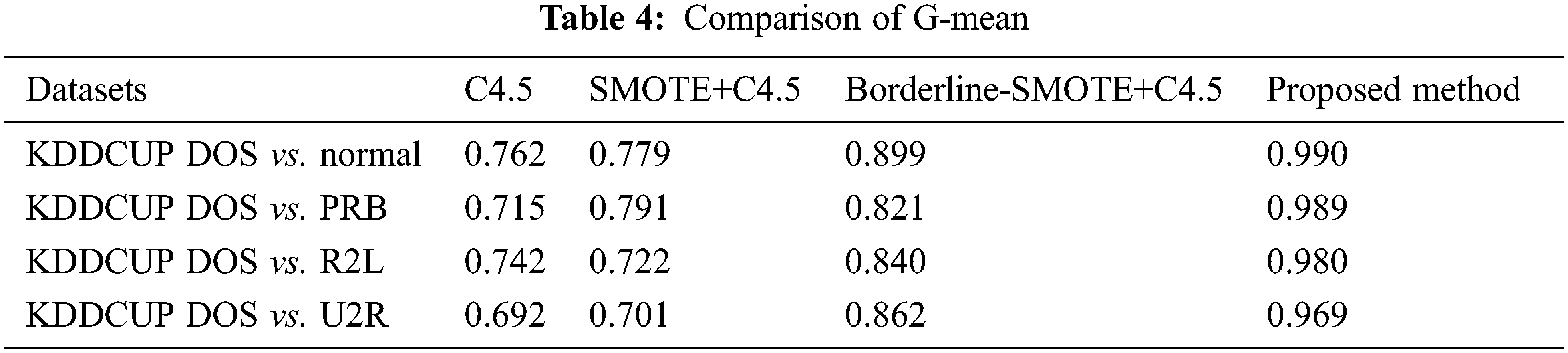
As shown in Tabs. 3 and 4, the suggested technique has been found to outperform the previous algorithms in terms of the classification performance. Across all four datasets, the proposed approach Hybrid SMOTE has been observed to achieve the maximum AUC value for the minority class classification performance. It has the highest G-mean value across all the datasets due to the suggested method’s usage of varying sampling rates for different minority class samples. Additionally, the hybrid SMOTE algorithm optimizes the sample rate mix. To utilize the other three techniques, you must specify a preset sampling rate for each of the dataset. If the value is set wrong, the classification performance of the algorithm would deteriorate. Additionally, the proposed hybrid algorithm self-adapts and intelligently determines the appropriate sampling rate combination for the dataset regardless of the changes in the sample size, attribute, unbalanced rate, and/or sample distribution. As a result, our method has achieved the best classification results in datasets with significant imbalances.

In all instances, increasing the number of mappers would result in a significant reduction in the construction time (Fig. 5). The G-Mean comparision is shown in Fig. 6. The Imbalanced Ratio (IR) affects the algorithm’s time consumption as it minimizes the negative class instances until they are equal in size to that of the positive class instances. As a result, we can see in Fig. 7 that the data sets with a greater imbalance ratio (R2L and U2R) takes longer to build than those with a lower imbalance ratio (normal and DOS), even though they have a larger number of instances. The experimental results show that the proposed method produces better results with the imbalanced datasets and reduces the class overlapping by selecting the optimal selection using a hybrid SMOTE algorithm. The MapReduce algorithm has used the parallel processing for handling large data sets with less building and classification time. The building time decreases as the number of mappers increases. Even thought he classification time increases as the number of mappers increases, the accuracy of the imbalanced data appears to be superior than that of the other classification methods.

Figure 5: AUC comparison

Figure 6: G-mean comparison

Figure 7: Building time against the number of mappers

5  Conclusion

In this paper, parallel processing for the hybrid SMOTE combination of SMOTE and Genetic Algorithm for overcoming the class overlapping and the imbalanced data set in big data has been proposed. By using the advantage of the MapReduce algorithm, our proposed method has performed well with the imbalanced big data set and essentially reduces the building time and the classification time. Our strategy has been divided into three stages. The first stage involves the use of a mapping function for dividing the data into smaller blocks, followed by a pre-processing step that employs a hybrid SMOTE algorithm for addressing the issues of class imbalance. Then, for each of the individual map blocks, a decision tree model has been built. The decision tree blocks have been combined for forming a classification model. According to the experimental results, our proposed method has been found to outperform the other SMOTE algorithms in the imbalanced classification in big data.

Funding Statement: The authors received no specific funding for this study.

Conflicts of Interest: The authors declare that they have no conflicts of interest to report regarding the present study.

This work is licensed under a Creative Commons Attribution 4.0 International License, which permits unrestricted use, distribution, and reproduction in any medium, provided the original work is properly cited.