DOI:10.32604/csse.2023.022938

| Computer Systems Science & Engineering DOI:10.32604/csse.2023.022938 |  |
| Article |
Music Genre Classification Using African Buffalo Optimization
1KPR Institute of Engineering and Technology, Coimbatore, 641407, India
2Government Engineering College, Palakkad, 678633, India
3Velammal Institute of Technology, Chennai, 601204, India
4Sathyabama Institute of Science and Technology, Chennai, 600119, India
*Corresponding Author: B. Jaishankar. Email: b.jaishankar@kpriet.ac.in
Received: 23 August 2021; Accepted: 02 March 2022
Abstract: In the discipline of Music Information Retrieval (MIR), categorizing music files according to their genre is a difficult process. Music genre classification is an important multimedia research domain for classification of music databases. In the proposed method music genre classification using features obtained from audio data is proposed. The classification is done using features extracted from the audio data of popular online repository namely GTZAN, ISMIR 2004 and Latin Music Dataset (LMD). The features highlight the differences between different musical styles. In the proposed method, feature selection is performed using an African Buffalo Optimization (ABO), and the resulting features are employed to classify the audio using Back Propagation Neural Networks (BPNN), Support Vector Machine (SVM), Naïve Bayes, decision tree and kNN classifiers. Performance evaluation reveals that, ABO based feature selection strategy achieves an average accuracy of 82% with mean square error (MSE) of 0.003 when used with neural network classifier.
Keywords: Genre; african buffalo optimization; neural network; SVM; audio data; music
The categorization of music genres sound is represented as an audio signal with characteristics such as frequency, decibel, and bandwidth. Amplitude and time can be used to communicate a typical audio stream. These audio signals are available in a variety of forms, making it possible for the computer to interpret and analyze them. The mp3 format, windows media audio (WMA) format, and waveform audio file (wav) format are only a few examples. Music categorization is used by businesses to provide suggestions to their customers or simply as a product. Identifying music genres is the initial step in performing either of the following two duties. One can use machine learning techniques to assist them do this. Music is differentiated by categorized classifications known as genres. Humans are the ones who come up with these genres. A music genre is defined by the features that its members have in common. These features are usually linked to the music's rhythmic structure, instrumentation, and harmonic content. In the subject of music information retrieval, which deals with viewing, organizing, and finding vast music collections, categorizing music files into their proper genres is a difficult issue. Genre categorization may help with a variety of interesting problems, such as creating song references, tracking down similar songs, finding societies that will appreciate that specific music, and even conducting surveys. Automatic musical genre categorization can assist or even replace humans in this process, making it a valuable addition to music information retrieval systems. Furthermore, automatic musical genre categorization may be used to generate and evaluate features for any form of content-based musical signal analysis. The notion of automated music genre classification has become quite popular in recent years due to the fast expansion of the digital entertainment sector. Although dividing music into genres is arbitrary, there are perceptual characteristics linked to rhythmic structure, instrumentation and texture of the music that can help to define a genre. Until now, genre classification for digitally downloaded music was done manually. Automatic genre categorization algorithms would thus be a valuable addition to the development of music audio information retrieval systems.
GTZAN dataset is a standard dataset for music genre classification. Blues, classical, Hip-hop, jazz, metal, reggae, pop, rock, disco and country are among the 10 genres included in the GTZAN dataset. Each class has 100 30-s recordings of music compositions. Compact CDs, Radio, and MP3 compressed audio files were used to create these snippets. Each item was saved as a mono audio file with a sample rate of 22.050 kHz and a bit depth of 16 bits [1,2].
The Music Technology Group built the ISMIR 2004 database to assist with various tasks in MIR. The MIR research community is attracted to this database in large numbers. It consists of six different styles of music: metal, classical, rock, electronic, blues, and world. The training and test sets are defined, and the distribution of music pieces per genre is not consistent. As a result, the artist filter will not work with this dataset. Both the training and test sets started off with 729 music pieces, bringing the total number of music pieces in the dataset to 1458. It was not feasible to use all of the music's in this dataset due to the signal segmentation method employed. It was feasible to employ just 711 of the 729 music pieces originally allotted to the training set. In the test set, 713 music pieces were utilized instead of 729.
The Latin Music Database (LMD) comprises 3227 full-length MP3 music samples derived from 501 artists’ compositions [2]. Forro, Axe, Bachata, Merengue, Bolero, Gau cha, Salsa, Pagode, Sertaneja and Tango are among the ten music genres represented in the database. One of the LMD's most distinguishing features is that it brings together a diverse range of genres that share considerable harmonic content, instrumentation and rhythmic structure. This is due to the fact that many of the genres in the database are from the same nation or countries with strong cultural connections. As a result, attempting to mechanically distinguish different genres is especially difficult. The music genre assignment in this database was done manually by a group of human specialists, based on human perceptions of how each piece of music is danced. The dataset is divided using an artist filter, which places all of an artist's music compositions in one fold and only one fold of the dataset [3].
To classify music, many characteristics that make up a song, such as top-level, mid-level, and low-level parts, have been defined. At the top of the list are human-defined categories including genre, mood, and artist. The pitch content aspects and rhythm characteristics such as beat and tempo are mid-level components that reflect the regularity of the music [4,5]. Low-level features are timbre characteristics derived from a short-time window such as 10–100 ms and used in speech analysis [6,7]. Some of the most often utilizedtimbre features are spectrum centroid/roll-off/flux, Mel-frequency cepstral coefficients (MFCC), octave-based spectral contrast [8], and time-varying characteristics like zero crossing and low energy [9]. The temporal development of the signal can be determined by combining the features taken from many frames to produce temporal features such as mean, variance, covariance, and kurtosis. The texture window is a lengthier window that is made up of frames [10–12].
For music genre categorization, representation learning vs. handmade features is proposed [13]. Audio and chords are two characteristics taken from two separate sources. Mel Frequency Cepstral Coefficients (MFCC), Statistical Spectrum Descriptors (SSD), and Robust Local Binary Patterns (RLBP) are the characteristics derived from audio. Simplified Chords Sequences is a feature taken from Chords (SCS). K-Nearest Neighbours (k-NN), Decision Trees (DT), Support Vector Machines (SVM), and Random Forest (RF) are the (BRMD) was employed, which includes algorithms used in the suggested system. BRazilian Music Dataset subgenres. The combination of learnt and handmade characteristics resulted in an accuracy of 78.15%, which was higher than the best individual CNN [2]. proposed a technique for music genre categorization based on timbral textural and pitch content characteristics. MFCC and other spectral properties make up timbral texture. The characteristics retrieved from chroma are chosen for the pitch content. Classical, country, disco, hip-hop, jazz, rock, blues, reggae, pop, and metal are among the 10 musical genres included in the GTZAN data collection. SVM, GMM, and k-NN are the classification methods utilized. The k-NN classifier achieves a classification accuracy of 69.7% utilizingtimbral textural and pitch content characteristics, respectively.
Classification of music genres using a multi-layer independent recurrent neural network (IndRNN) is proposed [14]. The scattering transform is the first step in the classification process, and it is used to pre-process the dataset with feature extraction. The data is then trained using a 5-layer architecture. The gradient disappearing and exploding problem is solved by IndRNN. The SoftMax classifier is ultimately employed as the classification algorithm. The Fourier coefficients or autocorrelation, which reflects the Mel spectrum process, are used in the modulation spectrum decomposition. The GTZAN dataset was utilized for the genre categorization. With a total training time of 0.23 s, IndRNN was able to attain a classification accuracy of 96%. A convolutional recurrent neural network is also to classify music genres. The convolution neural network was utilised as the algorithm. The datasets that were utilised were the GTZAN and MagnaTagATune databases. The MagnaTagATune dataset comprises 25,863 clips, each with a duration of around 29 s, derived from 5,405 mp3 songs. The clips in the GTZAN dataset are around 30 s long. Mel Spectrogram is a characteristic used to categorise music genres. On a 10-class genre categorization, the suggested model has an accuracy of 85.36%. The same model was trained and evaluated on the MagnaTagATune dataset's 10 genres, which totaled 18,476 clips with a length of 29 s. It is possible to obtain an accuracy of 86.06%. An audio-based categorization method for Indonesian dangdut music is proposed [15]. For music genre categorization, time-domain and frequency-domain audio characteristics are employed. The energy, entropy energy, and zero crossing rate are time-domain audio characteristics. The spectral centroid, spectral entropy, spectral flux, spectral roll-off, harmonic, MFCC and chroma vector are all frequency-domain audio characteristics. The classifier used for classification is the Support Vector Machine (SVM). 80 audio files for dangdut music and 80 audio files for techno dance music were utilized in the study. All of the audio recordings gathered are in MP3 format, with a sample rate of 44.1 kHz, stereo, and a song length of around four minutes. The suggested system employs SVM as a classifier. The collection of dangdut music and techno dance music is accurate to the tune of 80 percent to 90 percent.
The African Buffalo Optimization (ABO) was created to address the problems of existing algorithms such as low speed, premature convergence, the use of multiple parameters, and complicated fitness functions by ensuring that each buffalo's location is regularly updated and linked to the previous and current locations of the herd's best buffalo. African Buffalo Optimization (ABO) is an effort to create a user-friendly, robust, effective, efficient, and simple-to-implement algorithm that displays outstanding capability in the usage and inspection of the search area. The ABO algorithm is based on the buffalo's two warnings, ‘waaa’ and ‘maaa.’ The alert ‘waaa’ is used to mobilize buffalos to graze on a certain grazing tract. The alarm ‘maaa’ is used to communicate with the whole herd in order to find a better grazing spot. African buffalos utilize these vocalizations to organize themselves in the African woods in order to hunt the rich green pastures.
Each animal's location indicates a solution in the search space in this method. ABO provides quick convergence by using just a few parameters, the most important of which is the learning parameter. With only a few parameters, principally the learning parameters, ABO assures rapid convergence. The African Buffalo Optimization simulates the African buffalo's three distinct characteristics that enable them to find pastures. For starters, they have a large memory capacity. This allows the buffalos to follow their paths through thousands of kilometers of African terrain. The buffalos’ second characteristic is their capacity to cooperate and communicate in both good and bad circumstances. The ‘waaa’ cry is used to summon other buffalos to help other animals in distress. ‘Maaa’ vocalizations are used to tell the buffalo herd to stay there so they may take advantage of the current site, which promises rich grazing meadows and is safe. The buffalos’ third characteristic is their democratic nature, which is based on their high intellect.
ABO Process
Step 1: Objective function f(y) y = (y1, y2, …yn)
Step 2:Initialize by assigning buffalos to nodes in the solution space at random.
Step 3: Update the buffalo's fitness values
where wk and mk represents the exploration and exploitation moves respectively of the kth buffalo, lp1 and lp2 are learning factors; bgmax is the herd's, best fitness and bpmax is the individual buffalo's, best.
Step 4: Update the location of buffalo k
where λ is a unit of time
Step 5: Is bgmax updating. Yes, go to step 6. No, go to step 2
Step 6: If the stopping criteria is not met, go back to algorithm step 3, else go to step 7
Step 7: Output the best solution.
Fig. 1 shows the process flow of ABO. The Eq. (1) is divided into three parts, the first of which is the memory portion mk+1 which indicates that the animals are aware that they have migrated from their previous places mk to a new one. This demonstrates their large memory capacity, which is an important asset in their migratory lifestyle. The cooperative characteristics of the animals lp1 are represented in the second half lp1(bg max yk − wk). The last component of this equation lp2(bg max yk − wk) emphasize the animals’ extraordinary intellect. They can recognize the difference between their prior most productive location and their current one. As a result, they are better equipped to make educated judgments and hence the buffalos moves to a new place.
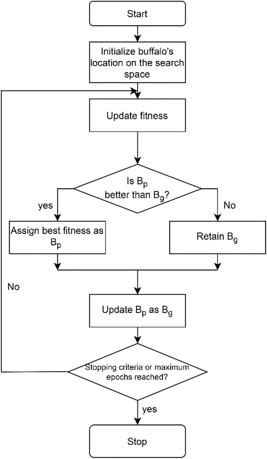
Figure 1: Process flow of African buffalo optimization
A windowing procedure is used to divide the continuous audio stream into smaller signal pieces in the suggested method. This is accomplished by sliding a window function, which results in a continuous succession of finite blocks of data. The audio signal is categorized as training and testing data. The audio signal subjected to feature extraction in which features are extracted from it. Among the features the dominant features are selection based on ABO algorithm. Fig. 2 shows the flowchart of the proposed method.
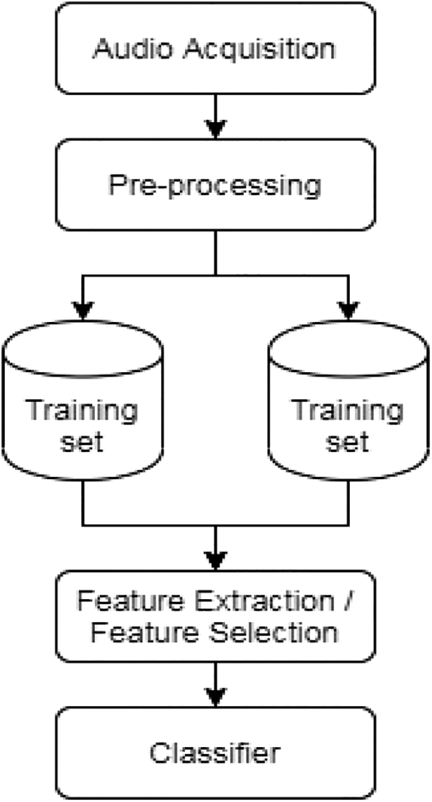
Figure 2: Process flow of the proposed method
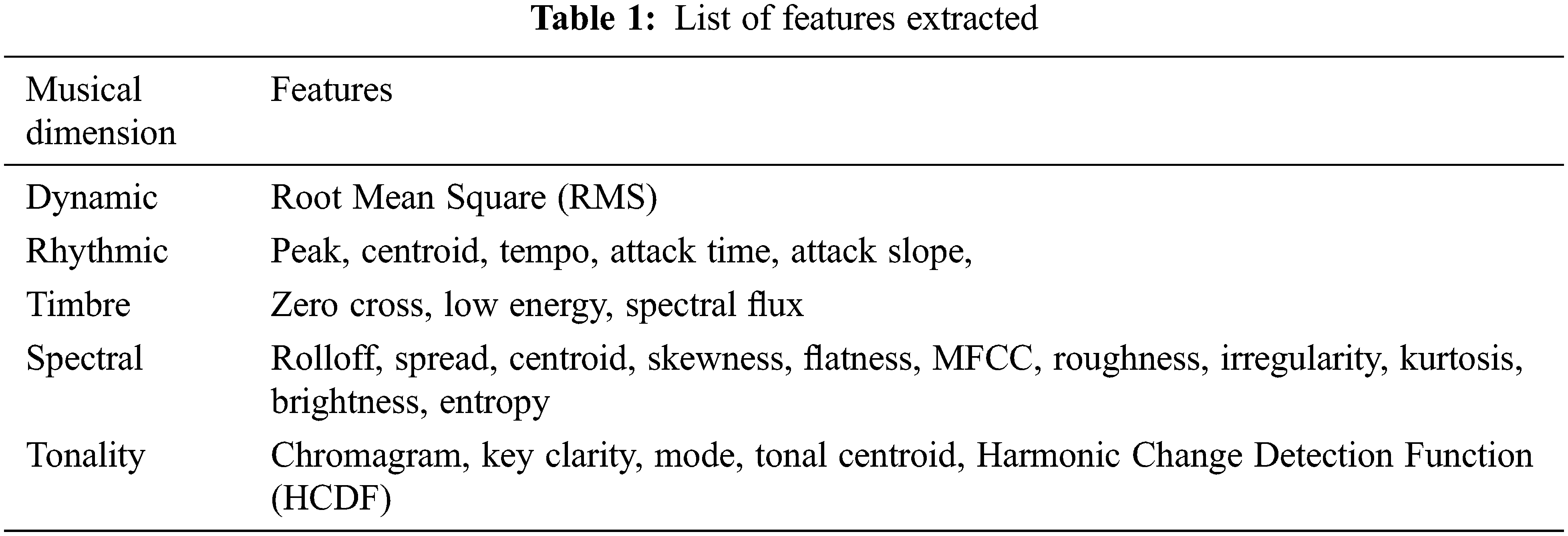
Instrumental music files from the GTZAN genre collection databases were used in this investigation. The information was gathered from the following sources: (i)the dataset consisted of 1000 30-s music files in a 16-bit mono audio format with a sampling rate of 22050 Hz. Blues, classical, country, disco, hip-hop, jazz, metal, pop, reggae, and rock were the ten musical genres assigned to the samples. Audio data files were used to acquire the raw data. Before doing feature extraction, the data were preprocessed by transforming the data files to a numerical format using MATLAB 2016b and the MIR toolbox. The tests were carried out on a typical laptop equipped with an Intel i5 CPU and 4 GB of RAM. For each frame, the musical characteristics in the different musical dimensions of dynamic, rhythmic, spectral, timbre, and tonal are retrieved. The mean and variance of these different audio features are computed, resulting in a total of 49 features for each sample audio. Out of 49 features, 2 features are under dimension dynamics. 10 features are under dimension rhythm which comprises of 5 mean features and 5 variance features. Considering mean and variance descriptors there exist 22 spectral features, five timbre features and ten tonal features.
To assess the performance of the classifier models, a tenfold cross validation was performed. One Vs All (OVA) classification is used in all classes. The accuracy and F-score are the performance measures used to evaluate the classifiers. The ratio of properly categorised examples to the total number of occurrences is known as accuracy. The ratio of accurately assigned class X samples to the total number of samples categorised as class X is known as precision. The ratio of properly allocated class X samples to the total number of samples in class X is known as recall. The geometric mean of accuracy and recall is the F score. The precision of a model is summarised by its exactness, whereas the recall of a model is summarised by its completeness. The F score is a superior descriptor for evaluating classifier performance. The geometric mean of accuracy and recall is used to get the F score. The F score is a number that ranges from 0 to 1. The higher the F-score, the better the classification performance. Fig. 3 shows the spectrum of the audio signal.
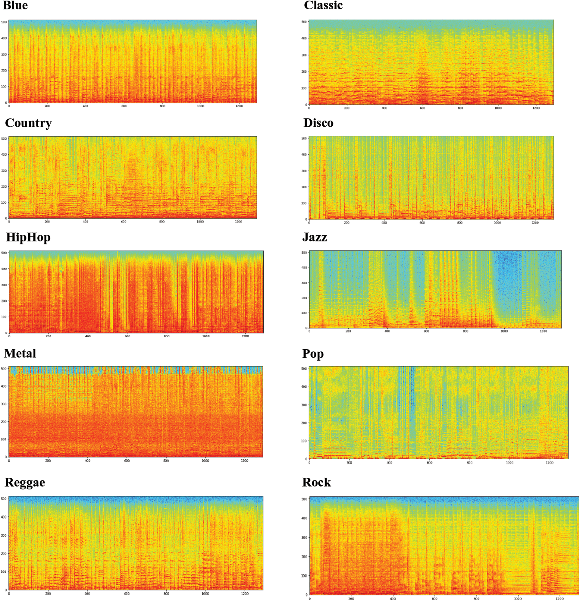
Figure 3: Sample spectrum of an audio signal
Five distinct classifiers are used to evaluate the classification performance of ABO-based feature selection:
1. Naïve Bayes classifier
2. Ginis diversity index, towing rule, and greatest deviation reduction are three criteria for a decision tree classifier. The classifier is put to the test with a number of splits ranging from one to one hundred.
3. kNN classifier with k = 1, 2, 3, 4 and for different distance metrics to assess the classifier.
4. Using the One against all method, SVM with linear, polynomial, quadratic, and Gaussian kernels (OVA strategy). One, two, or four characteristics determine the effectiveness of an SVM employing linear, Gaussian, or polynomial kernels, accordingly. The A hyper feature C is shared by all kernels and influences the performance of the SVM classifier. It's the constraint violation constant that tracks when a data sample is taken in the wrong part of the decision boundary. The width of the radial basis function is a feature σ (sigma) of the RBF kernel. The performance of the RBF-SVM classifier is determined by C and σ.
Grid-search and cross-validation errors with five-fold cross-validation are used to calculate the features C and σ. The degrees of the polynomial, the coefficient of the polynomial function, and the co-additive constant are denoted by d, γ, and a, respectively, for the polynomial kernel. The degree of the polynomial is changed while C is set to 1 and γ = (1/number of features).
5. 20 hidden layer neurons in neural network classifiers. Traingd, traingda, traingdm, traingdx, traincgf, traincgb, traincgp, trainlm, trainoss, trainrp, trainscg, trainbfg, and trainbr are among the 13 training algorithms used to create BPNN. The error goal is set at 0.01. The learning rate is varied between 0.01 and 0.9, while the momentum factor is changed between 0.01 and 0.9. Tan-sigmoid is the activation function utilised.
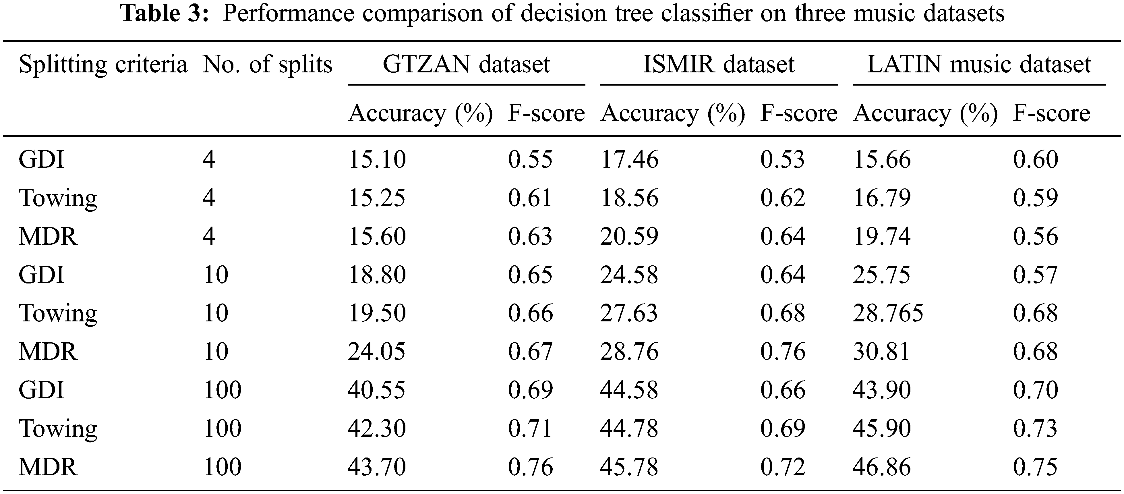
The list of features considered for analysis is shown in Tab. 1. Tab. 2 shows the classification accuracy of the Naïve bayes classifier in classifying the three musical dataset using the features selected using ABO. Naïve Bayes classifier yield classification accuracy of 12.20%, 15.46% and 18.70% for GTZAN, ISMIR, Latin Music datasets respectively for the features selected using the ABO optimization algorithm. Tab. 3 illustrates the performance of the decision tree classifier for three distinct splitting criterion: Gini's diversity index (GDI), towing, and Maximum deviance reduction (MDR), as well as for various numbers of splits ranging from one to one hundred. For the features selected using the ABO optimization algorithm, the tree classifier with hundred number of splits and splitting criteria of Maximum deviance reduction outperformed other tree classifiers with an average classification accuracy of 43.70 percent, 45.78 percent, and 46.86 percent for GTZAN, ISMIR, and Latin Music datasets, respectively. The classification performance of decision tree classifier is better compared to Naïve Bayes classifier.

The performance of the kNN classifier is shown in Tab. 4. For the characteristics picked using the ABO technique, the 1NN classifier classifies the music datasets better than the 2NN, 3NN, and 4NN classifiers among the kNN classifiers. All other kNN classifiers were surpassed by the INN classifier using Euclidean distance weight metric. The performance of the kNN classifier is shown in Tab. 4. For the characteristics picked using the ABO technique, the 1NN classifier classifies the music datasets better than the 2NN, 3NN, and 4NN classifiers among the kNN classifiers. All other kNN classifiers were surpassed by the INN classifier using Euclidean distance weight metric. The INN yield classification accuracy of 48.46%, 57.75% and 50.95% for GTZAN, ISMIR, Latin Music datasets respectively for the features selected using the ABO optimization algorithm. 1 NN classifier outperformed Naïve bayes classifier and decision tree classifier. Tab. 5 shows the performance of SVM classifier in classifying the musical datasets using the features selected using ABO. Of all the SVM classifier, the classifier with Gaussian kernel outperformed other kernels. Grid search and fivefold cross validation are used to find features C and sigma for the SVM classifier with Gaussian kernel. With the GTZAN, ISMIR, and LATIN music datasets, the classification performance of SVM with Gaussian kernel approaches 76.05 percent, 75.33 percent, and 76.55 percent, respectively, for as 0.1 and C as 1. Tab. 6 depicts the performance of a back propagation neural network classifier (BPNN) trained with a features subset chosen using the ABO technique. Tab. 6 shows the best classification accuracy of several training functions for various learning rates and momentum.


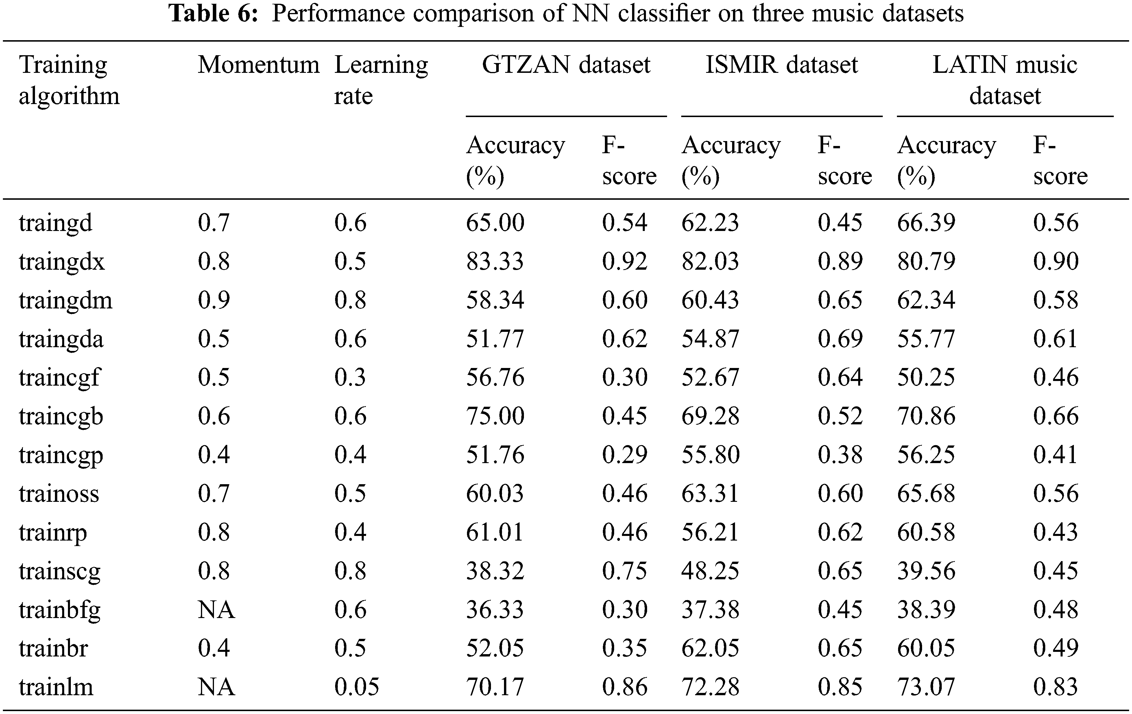
From Tab. 6, it is explicit that for the three music datasets, traingdx training algorithm yield maximum accuracy of 83.33%, 82.03% and 80.79%. traingdx gives maximum classification accuracy for learning rate of 0.5 and momentum of 0.8. NN classifier with the traingdx training algorithm yield F-score of 0.92, 0.89 and 0.90 respectively for GTZAN, ISMIR, Latin Music datasets respectively for the features selected using the ABO optimization algorithm. BPNN classifier outperformed all the classifier in classifying the musical datasets using the features selected using ABO. Also the F-score of this classifier is high compared to other classifiers signifying the high classification performance of BPNN classifier in classifying these musical datasets.
Fig. 4 summarize the performance of various classifiers on three datasets. NN classifier outperforms the other four classifiers in classifying the datasets using the features selected using ABO. NN classifier yield an average classification accuracy of nearly 82%. Next highest performance is exhibited by SVM classifier with average classification accuracy of nearly 76%.
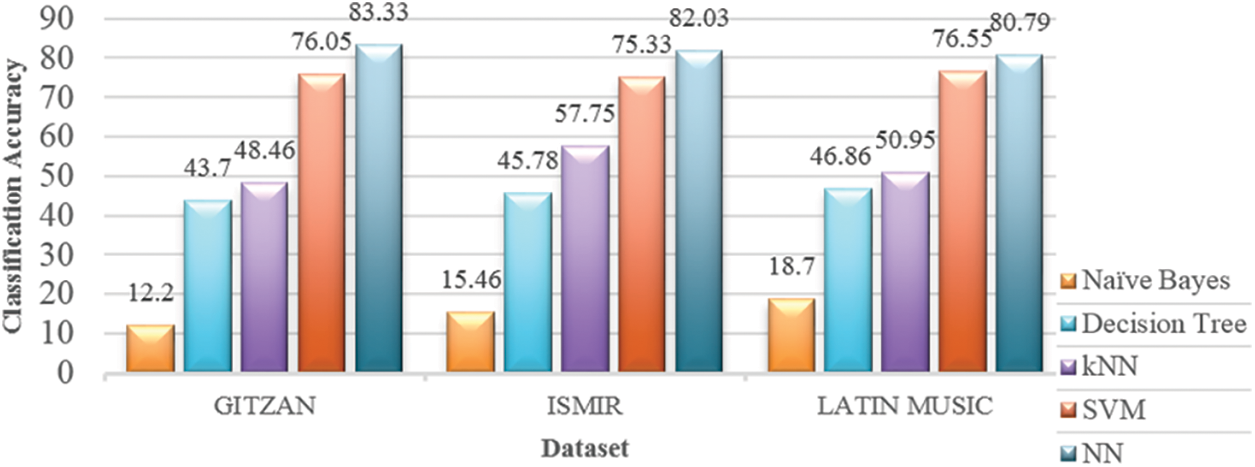
Figure 4: Performance of various classifiers
The kNN (k = 1) and Decision tree classifier gave average classification accuracy of 52% and 45% respectively. The Naïve Bayes classifier yielded the lowest classification accuracy of 15% only.
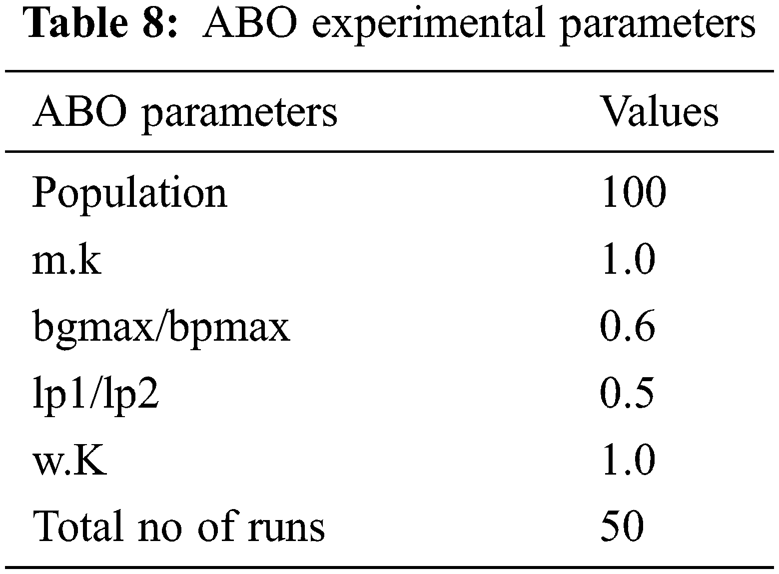
Tab. 7 shows the classification performance of the best two classifiers with the features selected with ABO on GTZAN dataset and without the feature selection. The classification is better using the feature selection algorithm. Tab. 8 shows ABO experimental parameters used in classification.

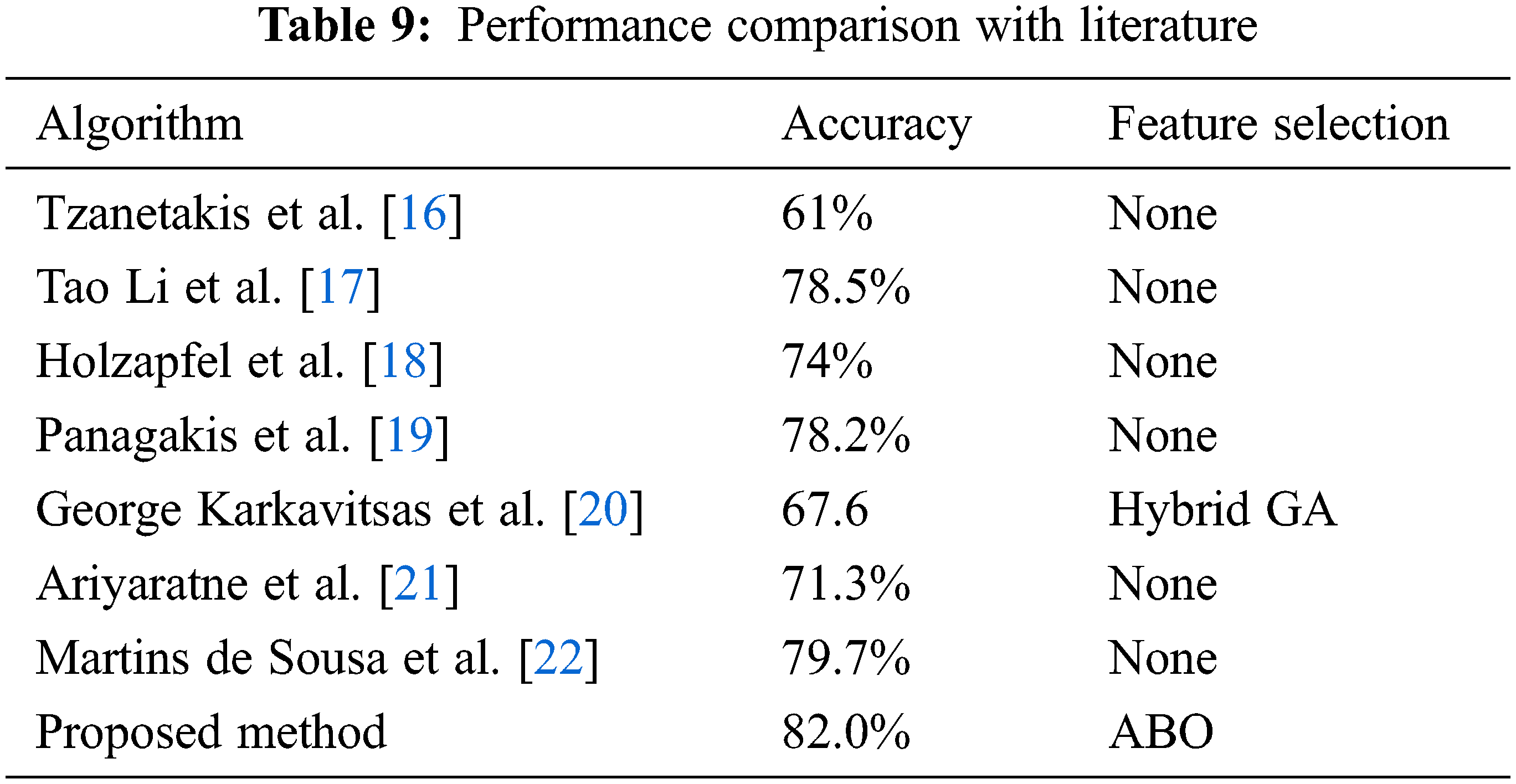
From Fig. 5, it is explicit that spectral features contribute nearly to 37%, 39% and 41% of the total features selected using ABO in three datasets respectively. The tonal feature is the next highest contributor in the feature subset followed by the timbre feature. The contribution by the rhythmic feature is least in all the three datasets. Tab. 9 shows the results obtained from the experiment with the African Buffalo Optimization (ABO) was compared with results obtained from similar experiments.
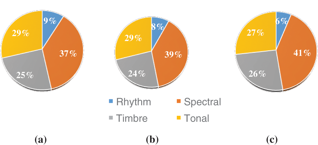
Figure 5: Percentage of musical features in feature subset selected using ABO (a) GTZAN (b) ISMIR (c) Latin Music
With the advent of internet and multimedia system applications that deal with the musical databases, the demand for music information retrieval applications has increased. Automatic analysis of musical database system extract important features from audio and classify the audio based on these features. Feature selection is inevitable in music data mining. In the proposed method, African buffalo optimization algorithm was used to select the best features to classify the music data for the benchmark datasets. Analysis shows ABO identify the relevant features and has immense capacity to obtain the solutions, with high accuracy and less error. An overall average accuracy of 82% is achieved when used with GTZAN, ISMIR and Latin Music dataset.
Funding Statement: The authors received no specific funding for this study.
Conflicts of Interest: The authors declare that they have no conflicts of interest to report regarding the present study.
1. S. Teh Chao Ying, S. Doraisamy and M. Lili Nurliyana Abdullah, “Genre and mood classification using lyric features,” in 2012 Int. Conf. on Information Retrieval & Knowledge Management, Kuala Lumpur, Malaysia, vol. 2, pp. 12, 2012. [Google Scholar]
2. T. Li, A. B. Chan and A. H. W. Chun, “Automatic musical pattern feature extraction using convolutional neural network,” in Proc. of the Int. Multi Conf. of Engineers and Computer Scientists 2010, Hong Kong, vol. 12, pp. 124, IMECS 2010. [Google Scholar]
3. M. Jakubec and M. Chmulik, “Automatic music genre recognition for in-car infotainment,” in Transportation Research Procedia, vol. 40, pp. 1364–1371, 2019. [Google Scholar]
4. J. Salamon and E. Gomez, “Melody extraction from polyphonic music signals using pitch contour characteristics,” in IEEE Transactions on Audio, Speech, and Language Processing, vol. 20, no. 6, pp. 1759–1770, 2012. [Google Scholar]
5. S. Tao Li and G. Tzanetakis, “Factors in automatic musical genre classification of audio signals,” in 2003 IEEE Workshop on Applications of Signal Processing to Audio and Acoustics (IEEE Cat. No.03TH8684), New Paltz, NY, USA, pp. 143–146, 2003. [Google Scholar]
6. Z. Fu, G. Lu, K. M. Ting and D. Zhang, “A survey of audio-based music classification and annotation,” Multimedia IEEE Transactions, vol. 13, no. 2, pp. 303–319, 2011. [Google Scholar]
7. O. Lartillot and P. Toiviainen, “A matlab toolbox for musical feature extraction from audio,” in Int. Conf. on Digital Audio Effects, Bordeaux, France, vol. 237, pp. 244, 2007. [Google Scholar]
8. S. Lim, J. Lee, S. Jang, S. Lee and M. Y. Kim, “Music-genre classification system based on spectro-temporal features and feature selection,” in IEEE Transactions on Consumer Electronics, vol. 58, no. 4, pp. 1262–1268, 2012. [Google Scholar]
9. S. Li, R. Ogihara, S. Mitsunori and M. Shenghuo, “Integrating features from different sources for music information retrieval,” in Proc.-IEEE Int. Conf. on Data Mining, ICDM, Hong Kong, China, vol. 13, pp. 372–381, 2006. [Google Scholar]
10. F. D. Shadrach and G. Kandasamy, “Neutrosophic cognitive maps (NCM) based feature selection approach for early leaf disease diagnosis,” Journal of Ambient Intelligence and Humanized Computing, vol. 12, pp. 5627–5638, 2021. [Google Scholar]
11. R. Anitha, K. Gunavathi and F. D. Shadrach, “Investigation on the musical features of carnatic ragas using neutrosophic logic,” in Journal of Physics: Conf. Series, India, vol. 1706, IOP Publishing Ltd, 2020. [Google Scholar]
12. R. Anitha and K. Gunavathi, “NCM-based raga classification using musical features,” International Journal of Fuzzy Systems, vol. 19, pp. 1603–1616, 2017. [Google Scholar]
13. R. M. Pereira, Y. M. G. Costa, R. L. Aguiar, A. S. Britto and L. E. S. Oliveira et al., “Representation learning vs. handcrafted features for music genre classification,” in Proc. of the Int. Joint Conf. on Neural Networks, Institute of Electrical and Electronics Engineers Inc., Budapest, Hungary, vol. 10, pp. 115, 2017. [Google Scholar]
14. W. Wu, F. Han, G. Song and Z. Wang, “Music genre classification using independent recurrent neural network,” in Proc. 2018 Chinese Automation Congress, Cac Institute of Electrical and Electronics Engineers Inc., Xi’an, China, pp. 192–195, 2018. [Google Scholar]
15. F. Mahardhika, H. L. Warnars, Y. Heryadi and V. Lukas, “Indonesian's dangdut music classification based on audio features,” in 1st 2018 Indonesian Association for Pattern Recognition Int. Conf., INAPR 2018–Proc., Institute of Electrical and Electronics Engineers Inc, Toronto, Canada China, pp. 99–103, 2019. [Google Scholar]
16. S. Tzanetakis, C. George and F. Perry, “Musical genre classification of audio signals,” IEEE Transactions on Speech and Audio Processing, vol. 10, pp. 293–302, 2002. [Google Scholar]
17. A. Tao Li, M. Mitsunori Ogihara and A. Qi Li, “A comparative study on content-based music genre classification,” in Proc. of the 26th Annual Int. ACM SIGIR Conf. on Research and Development in Informaion Retrieval, Toronto, Canada, vol. 15, pp. 282–289, 2003. [Google Scholar]
18. A. Holzapfel and Y. Stylianou, “Musical genre classification using nonnegative matrix factorization-based features,” IEEE Transactions on Audio, Speech, and Language Processing, vol. 16, no. 2, pp. 424–434, 2008. [Google Scholar]
19. I. Panagakis, E. Benetos and C. Kotropoulos, “Music genre classification: A multilinear approach,” In: J. P. Bello, E. Chew and D. Turnbull (Eds.) Int. Symp. Music Information Retrieval, Philadelphia, USA, vol. 2, pp. 583–588, 2008. [Google Scholar]
20. V. George Karkavitsas and A. George Tsihrintzis, “Automatic music genre classification using hybrid genetic algorithms,” in Intelligent Interactive Multimedia Systems and Services, vol. 1, pp. 323–335, 2011. [Google Scholar]
21. H. B. Ariyaratne and D. Zhang “A novel automatic hierachical approach to music genre classification,” in 2012 IEEE Int. Conf. on Multimedia and Expo Workshops, Melbourne, VIC, Australia, pp. 564–569, 2012. [Google Scholar]
22. J. Martins de Sousa, E. Torres Pereira and L. Ribeiro Veloso, “A robust music genre classification approach for global and regional music datasets evaluation,” in 2016 IEEE Int. Conf. on Digital Signal Processing (DSP), Beijing, China, pp. 109–113, 2016. [Google Scholar]
 | This work is licensed under a Creative Commons Attribution 4.0 International License, which permits unrestricted use, distribution, and reproduction in any medium, provided the original work is properly cited. |