DOI:10.32604/csse.2023.023728
| Computer Systems Science & Engineering DOI:10.32604/csse.2023.023728 | |
| Article |
Multiple Object Tracking through Background Learning
Jamia Millia Islamia, Department of Electrical Engineering, New-Delhi, 110025, India
*Corresponding Author: Deependra Sharma. Email: medeependrasharma@gmail.com
Received: 18 September 2021; Accepted: 14 December 2021
Abstract: This paper discusses about the new approach of multiple object tracking relative to background information. The concept of multiple object tracking through background learning is based upon the theory of relativity, that involves a frame of reference in spatial domain to localize and/or track any object. The field of multiple object tracking has seen a lot of research, but researchers have considered the background as redundant. However, in object tracking, the background plays a vital role and leads to definite improvement in the overall process of tracking. In the present work an algorithm is proposed for the multiple object tracking through background learning. The learning framework is based on graph embedding approach for localizing multiple objects. The graph utilizes the inherent capabilities of depth modelling that assist in prior to track occlusion avoidance among multiple objects. The proposed algorithm has been compared with the recent work available in literature on numerous performance evaluation measures. It is observed that our proposed algorithm gives better performance.
Keywords: Object tracking; image processing; background learning; graph embedding algorithm; computer vision
Multiple object tracking (MOT) is a crucial task in computer vision, with a wide range of tracking algorithms. Tracking and its complexity level depends on several factors, such as type of parameters being tracked namely size, contour, position, velocity, and acceleration. It may also depend on number of parameters used for tracking and the amount of prior knowledge about the target object. During tracking different situations may arise such as, tracking of mobile object appearing for the first time in the scene. When representations of the object under consideration are available, it is feasible to learn it for the first time. Object tracking is an act of seeking for objects in successive frames of a video stream after learning has been completed. Even after so much research, MOT remains a difficult work since the object’s appearance can radically vary due to deformation, rotation out of plane, or changes in lighting conditions. Problem becomes more challenging when tracking is to be done in dense places that consists of movable and immovable objects.
When faced handling problems including occlusions, illumination changes, motion blur, and other environmental changes, most existing techniques underperform [1]. To solve these issues, we present a background learning-based multiple object tracker. Even if background removal results in the identified objects being received as blobs, tracker can manage occlusions in a straight-through mode by using the relative background information of the object. In our case, the tracking being done with the knowledge of backdrop objects in the background, from which we can locate the foregrounds in the scenario. The principle of our approach is based on the theory of Relativity. It is widely known fact that to locate anyone’s position in a scene one must point out the objects relative to some fixed or moving object in that scene.
In this paper, we have combined background information with 3D mapping of foregrounds and proposed an occlusion-free model for multiple objects tracking in a complex scenario. As a result, designing a trained object detector that does not overlook objects is tough. We can get noisy candidate object locations by subtracting the background. To get an acceptable quality foreground object, we analyzed and processed each noisy candidate region. We use the background information model to generate a graph embedding tracker for each prospective region for localization. Objects that move in a sequential manner are localized and their states are updated frame by frame. A basic data relationship between background reference objects and to manage size variations, object fragmentation, occlusions, and lost tracks, background subtraction is used to find targets. Because both graph embedding technique and background removal could produce errors at numerous times, object states are determined utilizing the information from both. Finally, the system is tested using videos of pedestrians, moving automobiles, and other objects from various datasets. The benefits of adopting a robust visual tracker based on background information in a MOT framework are demonstrated by simulation results, which demonstrate that our technique is competitive even when data association is minimal.
The following is a breakdown of the paper’s structure: We address related work in part 2, and we show our proposed system in Section 3, which includes extracting ROIs, background subtraction, foreground analysis, and object tracking. In part 4, we put our method to the test and analyse the results. Finally, in part 5, we bring the paper to a conclusion.
Object detection has recently been prevailing paradigm in multiple object tracking. In this paradigm, object trajectories are commonly encountered in a global optimization problem that processes whole video batches at simultaneously. Flow network conceptions [2–4] and stochastic graphical models [5–8] are two examples of this sort of framework. These approaches, however, not suitable in online settings where a target identity needs to be provided at each time level owing to batch processing. Multiple Hypothesis Tracking (MHT) [9] and the Joint Probabilistic Data Association Filter (JPDAF) [10] are two more conventional approaches. These techniques work on a frame-by-frame basis to associate data. Individual measurements are weighted by their association likelihoods in the JPDAF to create a single state hypothesis. All potential hypotheses are tracked in MHT, however for computational tractability, pruning techniques must be used. The method has recently been re-examined in a tracking-by-detection situation [11], with encouraging results. An observation model based on a confidence score given through adding object-background prototypes into a discriminative model tries to handle occlusion well [12]. However, the additional computational and implementation complexity of these approaches comes with a cost.
Simple online and real-time tracking (SORT) [13] is a considerably simpler framework that inculcates Hungarian technique to conduct Kalman filtering in image space and frame-by-frame data association utilizing a bounding box overlap association measure. This straightforward method provides good results at high frame rates. SORT with a state-of-the-art person’s detector [14] outperforms MHT on standard detections on the MOT challenge dataset [15]. While the approach achieves generally strong tracking precision and accuracy, it also yields a very large number of identity changes due to prior-to-track occlusion management. Because by using the association metric can you be sure it’s accurate with the state estimate uncertainty is minimal, this is the case. As a result, most of the methods have trouble tracking around occlusions, which are common in camera with a frontal view situation. Did solve this problem via replacing the association measure with a more accurate metric that takes into account both motion and appearance. On a big-scale object re-identification dataset, we use a model network composed of relative background information that has been trained to identify foreground objects. We enhance resilience against misses and occlusions by integrating this network, while making the system simple to construct, efficient, and adaptable to online applications.
3 Proposed System for Multiple Object Tracking
The suggested system approach for multiple object tracking is depicted in Fig. 1 as a block diagram.
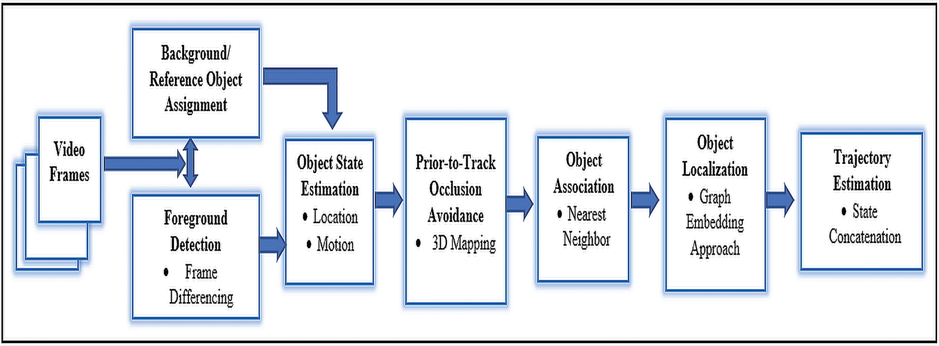
Figure 1: The proposed system approach is depicted as a block diagram
The proposed system methodology is being organized in a hierarchy manner as background/reference object assignment, multiple foreground detection, object association, state estimation, Prior-to-Track occlusion avoidance, object localization, and tracking.
The flow of the proposed system can well be understood with the help of visual description of various step involved as being done in Fig. 2 i.e., the pipeline of the proposed system approach.
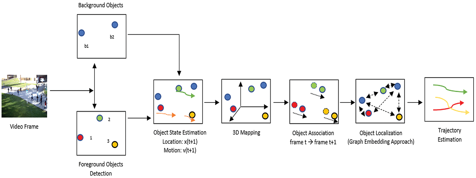
Figure 2: The suggested system approach’s pipeline
3.1 Background/ Reference Object Assignment
Taking background into consideration, in these the background is not subtracted from the frames with respect to the objects in the frame. Background reference points are a few significant stationary and/or moving elements in the background, gravitational centre is represented by centroids, giving us the location of those fixed backdrop objects. As in real science, we used to judge any objects positions with help of some reference objects in the background, so, using that thing in our research also, we will be predicting the new position of the moving object in the video.
In the Fig. 3 reference and three foreground objects are visible. The dash lines show the relative distances being computed between them at each frame and recorded for training the system.
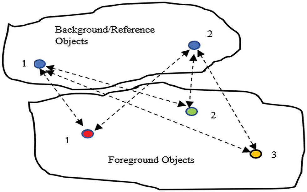
Figure 3: Background/ reference annotation
3.2 Foreground Object Detection
The frame differencing method being utilized for moving object detection. In the process, previous frame gets subtracted from the current frame followed by setting up appropriate threshold for moving object detection. The detected objects in the frame are being represented with the help of region properties as centroids and boundingbox, the boundingbox enclosing the object and the centroid representing the center of gravity of the detected object. In every scene, each centroid or detected object is represented with a particular node.
Graph theoretic approach: Centroid of the object represents x & y coordinates of the object’s position in the scene or frame this leads us to our first parameters in terms of the object’s location in the scene (x, y). Between the x co-ordinate and the frame number, a 2D plot is being drawn., showing trajectory of the different detected objects with the consecutive frames as shown in Fig. 4, random motion of the different detected objects can be seen in the figure. Similarly, 2D plot between y coordinate and frame number is shown in Fig. 4, which shows variation of y co-ordinate of the different detected objects with the consecutive frames. It is reflecting in figure that representing the detected objects with the center of gravity in the consecutive frames will lead to minimum variation in y coordinate with respect to its initial values.
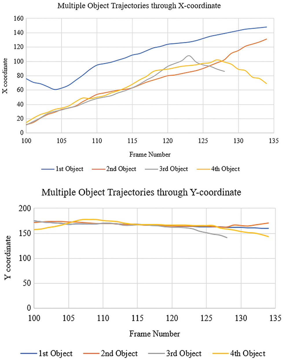
Figure 4: Multiple object trajectories through x and y co-ordinates
Combination of x & y co-ordinate trajectories as 2D plot between x & y co-ordinates shown in Fig. 5, the figure describes real scenario of video comprising of different detected objects motion paths. The disadvantage of this plot is that the different objects paths are being overlapped by some other detected objects path in the same scenario i.e., occlusion occurs and only few objects path can be interpreted correctly. So, to avoid occlusion the 3D reconstruction is done of the real scenario with the help of estimation of 3D parameters.
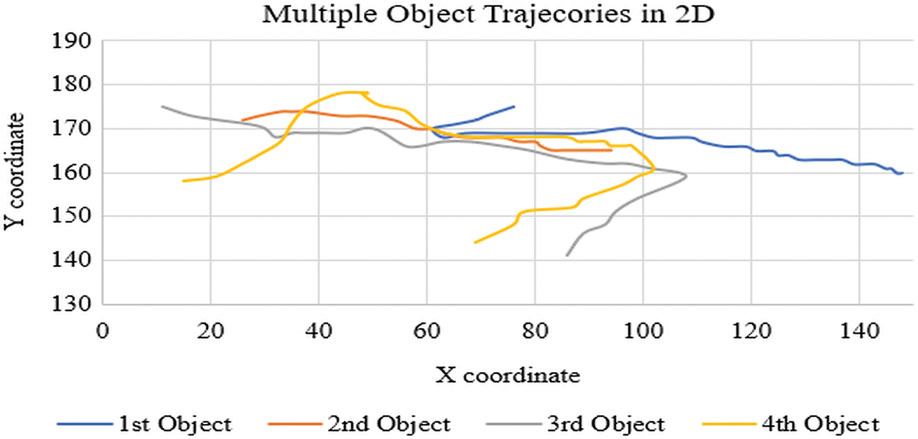
Figure 5: Multiple object trajectories in 2D
As all objects are represented with centroids having different x & y co-ordinates according to their position, relative distances are calculated between each centroid in the scene or frame with respect to the camera leading us to our second parameter in terms of distances between the objects of the scene or frame. A Tensor is prepared which comprises of these parameters for each frame, from where the parameter data can be retrieved for further processing. With the help of the framerate of video and the computed relative distances the third parameter is evaluated as speed, along with the direction of movement of each object the velocity vector is putted as another parameter in the tensor.
3.4 Prior-To-Track Occlusion Avoidance: Depth Modelling
Measurement of depth of the whole scenario in terms of the object placements referred to as the depth model. The Fig. 6 depicts the depth modeling of the scenario comprising of objects at different locations or different distances from camera.
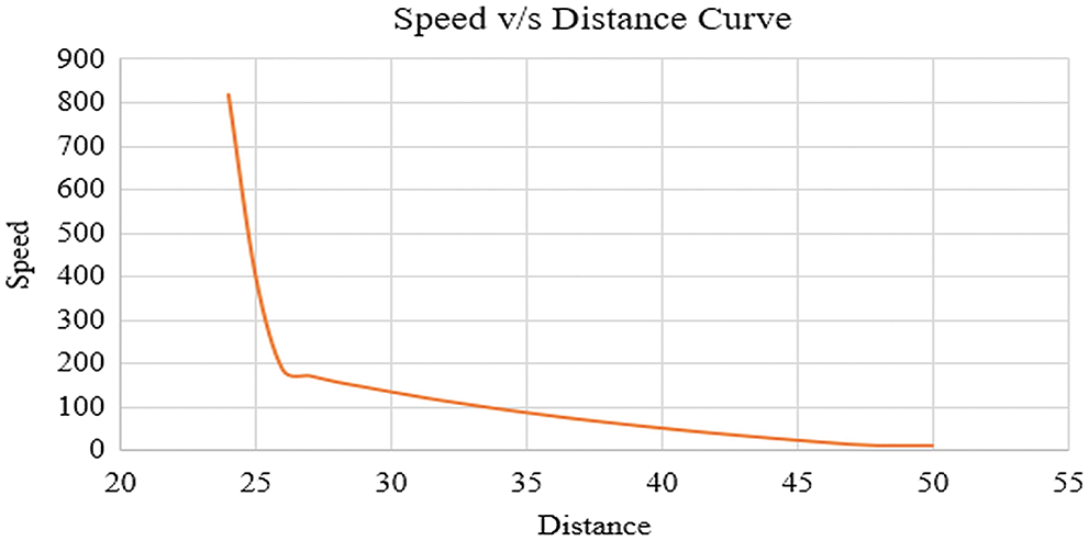
Figure 6: Depth modelling principle
The model describes the variation in speed of an object with respect to the camera. It explains the non-linearity that the object which is near to a camera it seems to be faster in comparison to an object which is much far from the camera, the far one will appear as slower with respect to camera. In the real scenario the object which is far and another which is near to camera will move at same speed, but with respect to camera the speed varies with distance, that we have proved in the depth model. With this depth model we can have an estimate of the object position in that scenario, i.e., the slower object will occupy the far position and the fast object will occupy the least position or near to camera.
So, for all the frames these three parameters are computed for the tensor and this tensor is being referred to as 2D data or 2D parameters. Then with the help of 2D data from the tensor, the 3D plot is drawn between x co-ordinate, y co-ordinate & the relative distances respectively along the 3 axes of the 3D plot as shown in Fig. 7, the figure also describes that the object paths do not occlude with each other as in case of 2D, so occlusion is removed. Each node in the 3D plot represents an object and has three pieces of information: x, y, and distance between them. Monocular vision or a single static camera are used to create a 3D picture of the position of the objects in the scene and rebuild it. Now, for each frame a 3D plot is being constructed.
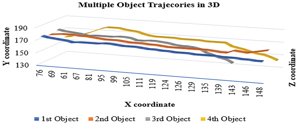
Figure 7: 3D mapping of multiple object trajectories
With all the 3D plots corresponding to all frames, again the three 3D parameters are computed in the terms of three-dimensional state and motion.
Each object or node is recognized from current frame to next frame the frame with the help of nearest neighbor classification, in which the minimum statistical distance is being calculated between the nodes in current frame with respect to the previous frame. Sequence of the visited nodes by the current node is output of the algorithm. Implementation of nearest neighbor algorithm is easy and execution time is also very less. The definition of statistical distance: hypothesis before the first k times scanning, we have established the N1 path. New observations for the first k times is Z j (k), j = 1, 2,.., N1. In the association gate of track i, the difference vector of observed j and track i is defined as the difference between the measured value and predicted value, the filter residue [16],
where H is the observation matrix, let S(k) be the covariance matrix. Then the statistical distance (square) being,
It is the judgment of nearest neighbor points metrics.
Recent research shows that graph embedding techniques [17] have enormous capacity of transforming high-dimensional sparse graphs into low-dimensional, dense vector spaces as shown in Fig. 8, where the graph structure properties are maximally preserved [18]. The generated nonlinear and highly informative graph embeddings in terms of features in the latent space can be conveniently used to address different downstream graph analytic tasks i.e., object classification, object state prediction, etc. The main objective of graph embedding method being to encode object states into a latent vector space, i.e., pack every object state’s parameter into a vector with a smaller dimension. Hence, various object state’s parameter related estimations in the original complex irregular spaces can be easily quantified based on various measures in the embedded vector spaces. Furthermore, the learned latent embeddings can greatly support much faster and more accurate graph analytics as opposed to directly performing such tasks in the high-dimensional complex graph domain. Graph embedding is a type of graph design that has certain unique restrictions. Nie et al. offer a graph-embedding framework for dimension reduction in [19], which graph-embeddingizes conventional PCA and FDA. The capabilities of graph approaches have also been exploited by [20–22] for various learning tasks. We present graph-embedding-based technique for successfully learning the variational appearances and discriminative structure between target object and the background, which is inspired by their work.
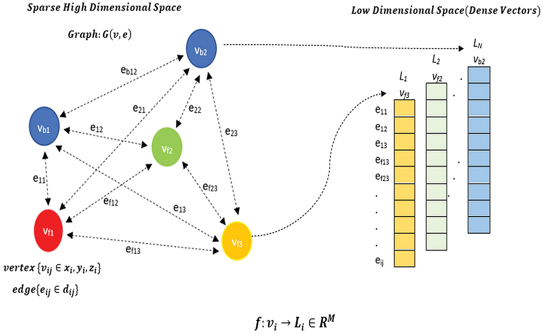
Figure 8: Schematic of graph embedding approach for a graph G(v,e)
3.6.1 Mathematical Formulation of the Graph Embedding Problem
In this section, we first present some preliminary graph notations, definitions and properties used in graph embedding. Then, we will define the object state measures applied in graph embedding.
Considering the weighted graph G(v,e) given in Fig. 8. As a mathematical data structure that contains an object’s state as node (or vertex) set v = {v1 , v2 , v3 , …, vn } and Euclidean distance between two nodes as edge (or link) set e. In the edge set, one edge eij describes the connection between two different nodes vi and vj, hence, eij can be represented as (vi , vj ), where vi , vj ∈ v, and nodes vi and vj are adjacent nodes. Low dimensional incidence dense vectors: It employs a | e| column vector to represent the relationship between object state set and distance edge set in a graph for the current frame. G(v,e) consisting of a node set v and an edge set e, using a graph embedding model f, different nodes (e.g., vb1 and vf2) from the original graph in a high-dimensional domain can be mapped into a latent low-dimensional space as a M-dimensional dense vector Li, M<< |v|. The node structure property can be also preserved in the latent space, i.e., similar nodes in the original space will be close to each other in the latent space. Moreover, the obtained latent variables Li, i ∈ v (i.e., features) can be readily used for diverse downstream graph analytic tasks. More details can be seen in Fig. 8, where each column denotes different object’s state, and each row denotes various distance edge set in a weighted graph. Each element in the vector can be filled with the relative distances respective to the concerned object.
3.6.3 Graph Embedding Problem Setting
In line with the aforementioned graph notations and definitions, given a graph G(v, e), the task to learn its graph object state node embeddings (e.g., M dimension, M << |v|) can be mathematically formulated as learning a projection φ, such that all graph object state nodes ( v = {vi |i = 1, 2, …, |v|}) can be encoded from high-dimensional space into a low-dimensional space, object state node embedding form being the deterministic point vectors (φ = {Li ∈ RM |i = 1, 2, …, |v|}).
The main purpose of vector point-based graph embedding is to project high-dimensional graph object state nodes (vi) into low-dimensional vectors (Li) in a latent space (RM), while preserving the original graph structure properties, with the mathematical function f as,
Graph G(v, e) contains the various information about the variational appearances and discriminative structure between background and multiple objects being target. The background and target object’s state being represented as location and motion in the form of three-dimensional coordinates. Object location contained through vertex vij in state s as,
Relative distances between objects expressed through edge eij containing the difference between the visit and the past node state as,
Combination of the vertex v and edges e will lead to the weighted graph representing the frame features at spatial instance t,
Each frame Graph
The object location state(s) in next frame t+1 could be measured through the previous state incidences in consideration with the time per frame tpf as,
The object motion state(a) in frame t could be measured through the previous and current state incidences in consideration with the time per frame tpf as,
In case of occlussion, the object state can still be estimated by the system precisely as the system being considering the depth information of all the objects present in the frame either moving/stationary or the foreground/background objects. Mathematical formultion for object state estimation in terms of location (s) and motion (a) for the current frame can be done through,
With the help of these vectorization of weighted graph models in terms of item location and motion for subsequent frames, a collaborative forecast is being made.
The state of each object in frame being evaluated in the above steps and now they are concatenated in a form that it forms a continuous trajectory (arising/ vanishing) for every object.
The proposed system is simulated using MATLAB software version R2020b. The hardware used for the simulation is Intel Core i5 1035G1 with 4 GB RAM and clock speed up to 3.6 GHz. The training and testing dataset used as described in Tab. 1.
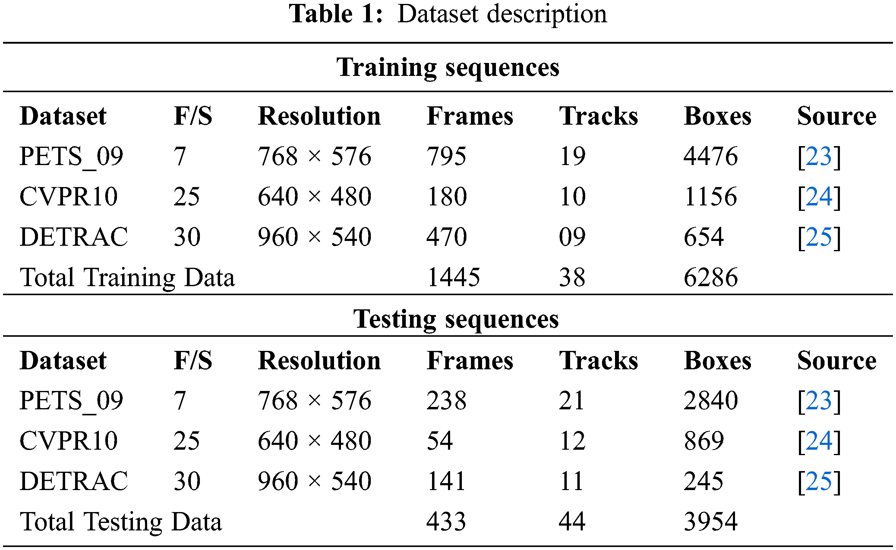
Fig. 9 illustrates some of the data used for tracking the objects with background reference points for all the three datasets given in Tab. 1.
With the proposed system approach, it is proven that tracking is better when the background of the scenario is taken into consideration rather than background subtraction as it is done mainly in the conventional tracking methods. In Fig. 9, few sample data have been shown. It depicts the tracked object in various samples of frame along the time, with tracking relatively with the reference objects in the background, the reference objects can be fixed or movable; in our case it is fixed, where the tracking is better or we could say nearly perfect whereas in the other category i.e., without considering the background, it suffers in terms of imperfect tracking as depicted in majority of the other state of art algorithms. So, increasing overall correctness of the system in terms of tracking will mainly depend on the consideration or rejection of the background of the scenario, which is proven by our system.
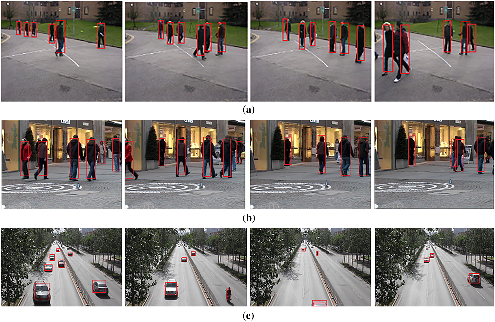
Figure 9: Various dataset showing the tracking of objects with the consideration of the background reference points (a) PETS09 Dataset, (b) CVPR10 Dataset, (c) UA_DETRAC Dataset
4.1 Performance Evaluation Criterion
Many measures have been developed in the past for evaluating multiple target tracking quantitatively. The proper one depends heavily on the application, and the search for a single, universal evaluation criterion is currently underway. On one side, it being ideal to condense results into a single number that can be compared directly. On the other side, one could not want to lose knowledge about the algorithms’ specific faults and present a large number of performance estimations, which makes a clear voting impossible. There are two common conditions for evaluating a tracker’s performance. The first step is to assess whether every postulated output being a true positive (TP) that describes an actual goal or a false alarm or false positive (FP). Thresholding based on a set distance is commonly used to make this decision (or dissimilarity). A false negative is a target that any hypothesis misses. It being assumed that good result will have as few FPs and FNs as possible. Also displayed false positive ratio, which is calculated using the count of false alarms with each frame (FAF), which is too known as false positives per image (FPPI) as mentioned in object detection literature. It’s understandable that many outputs may cover the same target. Before counting the numbers, second step being to establish correspondence through all annotated and hypothesized objects, keeping in mind that a true item should only be retrieved once, and that one hypothesis cannot account for more than one target. Because it is difficult to evaluate multitarget tracking performance with a single score, we combine the evaluation criteria defined in [26] with the conventional MOT metrics [23]:
4.1.1 Multiple Object Tracking Accuracy (MOTA)
This metric considers three different types of errors: false positives, missed targets, and identity changes. For improved tracking accuracy, a high MOTA value is preferred. The MOTA is arguably the most used metric for assessing the performance of a tracker. The major reason for this is that it is expressive, as it mixes three types of errors:
The frame index is t, and the count of ground truth objects is GT. MOTA could be negative if count of mistakes produced by tracker is more than total object count in the scene. MOTA score being solid indicator of tracking system’s overall performance.
4.1.2 Multiple Object Tracking Precision (MOTP)
Refers to average difference between all true positives and their ground truth objectives. For improved tracking, a high MOTP value is preferred. Average dissimilarity among all true positives and their matching ground truth targets is Multiple Object Tracking Precision. This being calculated as, for bounding box overlap:
dt,i is the bounding box overlap of target i with its assigned ground truth object, and ct is count of matches in frame t. Average overlap among all properly matched hypotheses and their corresponding objects being given by MOTP, which spans among td: 50% and 100%.
In ground truth, count of correctly matched detections being divided by total count of detections. A high value of recall is desirable for better tracking.
4.1.4 False Alarms per Frame (FAF)
It reflects per-frame number of false alarms. A lower value of FAF is desirable for better tracking.
It indicates the number of paths that have been mainly tracked. i.e., the target has had the same label for at least 80% of its existence. A high value of MT parameter is desirable for better tracking.
It indicates the number of trajectories that have been lost for the most part. i.e., the target being not monitored for at least 20% of the time it is alive. A lower value of ML parameter is desirable for better tracking.
It reflects number of false detections. A lower value of FP parameter is desirable for better tracking.
It reflects number of missed detections. A lower value of FN parameter is desirable for better tracking.
4.2 Performance Evaluation of the Proposed System
Each ground truth trajectory is divided into two categories: mainly tracked (MT) and mostly lost (ML). That being determined by the trajectory count, the tracking algorithm being able to retrieve. If a target being effectively tracked for at least 80% of its life cycle, it is considered mostly tracked. It’s worth noting that whether their identity remains the same throughout the track has no bearing on this measurement. A track is said to be ML if it is only restored for less than 20% of its overall length. The remaining tracks are only partially tracked. It is preferable to have more MT and fewer ML. The ratio of MT and ML targets to total number of ground truth trajectories is used to calculate MT and ML.
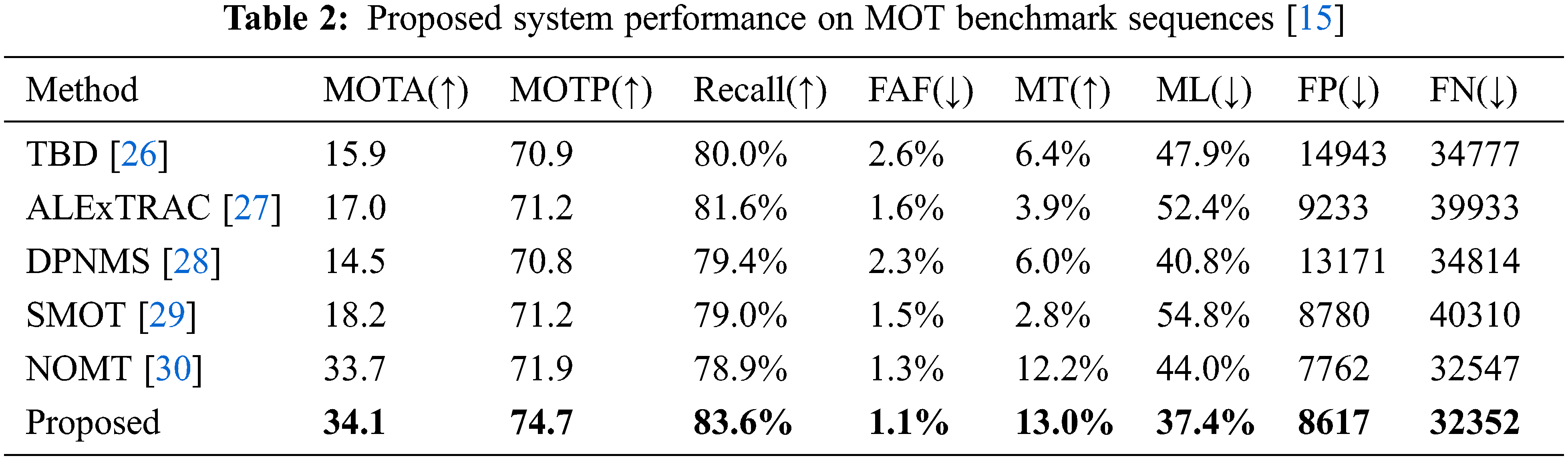
The graphical representation of the evaluated parameters as shown in Tab. 2 is depicted in Fig. 10.
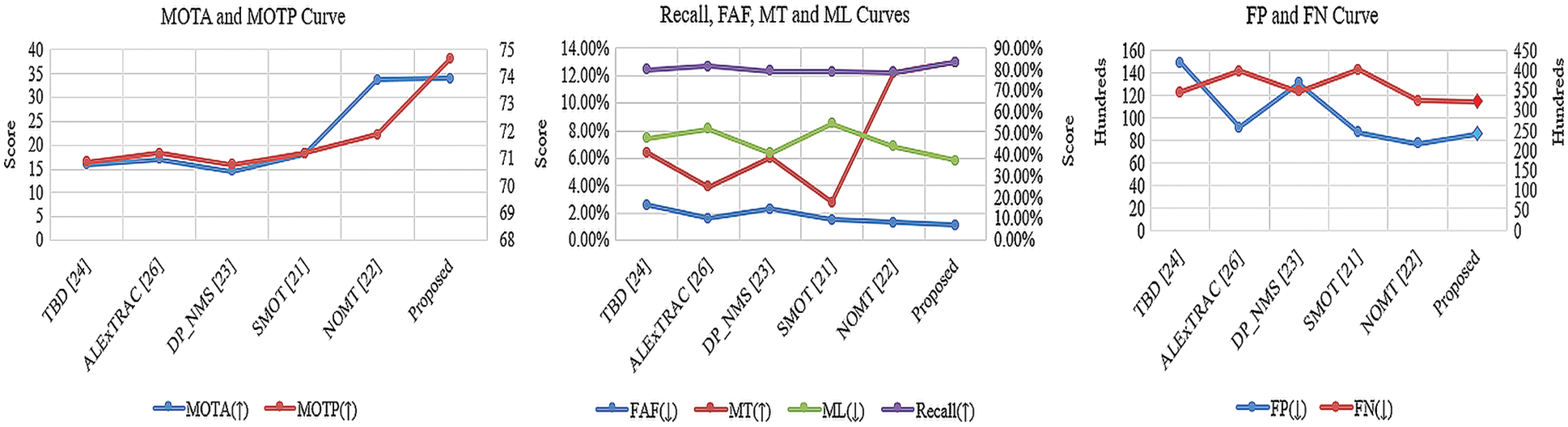
Figure 10: Performance measure curves of proposed system approach with state of art approaches
In this paper, we describe a unique tracking system that focuses on frame-to-frame forecast and occlusion management. When creating the system, it was assessed that an object’s tracking accuracy is heavily dependent on the relative information of surrounding objects, which might be fixed or moving. The suggested system’s performance is assessed and compared to existing traditional tracking methods available in the literature. The simulation result exhibits that the proposed framework achieves better parameter scores in terms of high accuracy, precision and recall rate as given in Tab. 2. At the same time the proposed system gives low scores for false alarms per frame, lost trajectories, number of false and missed detections, that indicates the superiority over other methods.
Funding Statement: The authors received no specific funding for this study.
Conflicts of Interest: The authors declare that they have no conflicts of interest to report regarding the present study.
1. S. A. Ahmed, D. P. Dogra, S. Kar and P. P. Roy, “Trajectory-based surveillance analysis: A Survey,” Circuits and Systems for Video Technology, vol. 29, no. 7, pp. 1985–1997, 2019. [Google Scholar]
2. V. Chari, S. L. Julien, I. Laptev and J. Sivic, “On pairwise costs for network flow multi-object tracking,” in Proc. IEEE Conf. on Computer Vision and Pattern Recognition, Boston, MA, USA, pp. 5537–5545, 2015. [Google Scholar]
3. S. Schulter, P. Vernaza, W. Choi and M. Chandraker, “Deep network flow for multi-object tracking,” in Proc. IEEE Conf. on Computer Vision and Pattern Recognition, Honolulu, HI, USA, pp. 2730–2739, 2017. [Google Scholar]
4. A. Hornakova, R. Henschel, B. Rosenhahn and P. Swoboda, “Lifted disjoint paths with application in multiple object tracking,” in Proc. Int. Conf. on Machine Learning, Online, PLMR, pp. 119–141, 2020. [Google Scholar]
5. M. Khaledyan, A. P. Vinod, M. Oishi and J. A. Richards, “Optimal coverage control and stochastic multi-target tracking,” in Proc. IEEE Conf. on Decision and Control, Nice, France, pp. 2467–2472, 2019. [Google Scholar]
6. Á.F. García-Fernández, L. Svensson and M. R. Morelande, “Multiple target tracking based on sets of trajectories,” Aerospace and Electronic Systems, vol. 56, no. 3, pp. 1685–1707, 2020. [Google Scholar]
7. S. Panicker, A. K. Gostar, A. Bab-Hadiashar and R. Hoseinnezhad, “Recent advances in stochastic sensor control for multi-object tracking,” Sensors, vol. 19, no. 17, pp. 3790, 2019. [Google Scholar]
8. S. Wang, Q. Bao and Z. Chen, “Refined PHD filter for multi-target tracking under low detection probability,” Sensors, vol. 19, no. 13, pp. 2842–2854, 2019. [Google Scholar]
9. K. Yoon, Y. Song and M. Jeon, “Multiple hypothesis tracking algorithm for multi-target multi-camera tracking with disjoint views,” IET Image Processing, vol. 12, no. 7, pp. 1175–1184, 2018. [Google Scholar]
10. S. He, H. Shin and A. Tsourdos, “Joint probabilistic data association filter with unknown detection probability and clutter rate,” in Proc. IEEE Int. Conf. on Multisensor Fusion and Integration for Intelligent Systems, Daegu, Korea (Southpp. 559–564, 2017. [Google Scholar]
11. S. H. Rezatofighi, A. Milan, Z. Zhang, Qi. Shi, A. Dic et al., “Joint probabilistic data association revisited,” in Proc. IEEE Int. Conf. on Computer Vision (ICCV), Santiago, Chile, pp. 3047–3055, 2015. [Google Scholar]
12. A. Mondal, “Occluded object tracking using object-background prototypes and particle filter,” Applied Intelligence, vol. 51, no. 1, pp. 5259–5279, 2021. [Google Scholar]
13. A. Bewley, G. Zongyuan, F. Ramos and B. Upcroft, “Simple online and realtime tracking,” in Proc. IEEE Int. Conf. on Image Processing (ICIP), Phoenix, AZ, USA, pp. 3464–3468, 2016. [Google Scholar]
14. S. Ren, K. He, R. Girshick and J. Sun, “Faster R-CNN: Towards real-time object detection with region proposal networks,” IEEE Transactions on Pattern Analysis & Machine Intelligence, vol. 39, no. 6, pp. 1137–1149, 2017. [Google Scholar]
15. L. Leal-Taix´e, A. Milan, I. Reid, S. Roth and K. Schindler, “MOT Challenge 2015: Towards a benchmark for multi-target tracking,” ArXiv, 2015. [Online]. Available: https://arxiv.org/abs/1504.01942. [Google Scholar]
16. K. Taunk, S. De, S. Verma and A. Swetapadma, “A brief review of nearest neighbor algorithm for learning and classification,” in Proc. Int. Conf. on Intelligent Computing and Control Systems (ICCS), Madurai, India, pp. 1255–1260, 2019. [Google Scholar]
17. H. Cai, V. W. Zheng and K. C. C. Chang, “A comprehensive survey of graph embedding: Problems, techniques, and applications,” IEEE Transactions on Knowledge and Data Engineering, vol. 30, no. 9, pp. 1616–1637, 2018. [Google Scholar]
18. P. Goyal and E. Ferrara, “Graph embedding techniques, applications, and performance: A survey,” Knowledge-Based Systems, vol. 151, no. 1, pp. 78–94, 2018. [Google Scholar]
19. F. Nie, Z. Wang, R. Wang, Z. Wang and X. Li, “Adaptive local linear discriminant analysis,” ACM Transactions on Knowledge Discovery from Data, vol. 14, no. 1, pp. 1–19, 2020. [Google Scholar]
20. A. Geiger, M. Lauer, C. Wojek, C. Stiller and R. Urtasun, “3D traffic scene understanding from movable platforms,” IEEE Transactions on Pattern Analysis and Machine Intelligence, vol. 36, no. 5, pp. 1012–1025, 2014. [Google Scholar]
21. S. Kamkar, F. Ghezloo, H. A. Moghaddam, A. Borji and R. Lashgari, “Multiple-target tracking in human and machine vision,” PLOS Computational B, vol. 16, no. 4, pp. 1–28, 2020. [Google Scholar]
22. M. Kumar and R. Gupta, “Overlapping attributed graph clustering using mixed strategy games,” Applied Intelligence, vol. 51, no. 8, pp. 5299–5313, 2021. [Google Scholar]
23. J. Ferryman and A. Ellis, “PETS2010: Dataset and challenge,” in Proc. IEEE Int. Conf. on Advanced Video and Signal Based Surveillance, Boston, MA, USA, pp. 143–150, 2010. [Google Scholar]
24. M. Andriluka, S. Roth and B. Schiele, “Monocular 3D pose estimation and tracking by detection,” in Proc. IEEE Computer Society Conf. on Computer Vision and Pattern Recognition, San Francisco, CA, USA, pp. 623–630, 2010. [Google Scholar]
25. L. Wen, D. Du, Z. Cai, Z. Lei and Ming, “UA-DETRAC: New benchmark and protocol for multi-object detection and tracking,” Journal of Computer Vision and Image Understanding, vol. 19, no. 3, pp. 634–654, 2020. [Google Scholar]
26. P. Dendorfer, H. Rezatofighi, A. Milan, J. Shi, D. Cremers et al., “A benchmark for multi object tracking in crowded scenes,” ArXiv, 2020. [Online]. Available: https://arxiv.org/pdf/2003.09003. [Google Scholar]
27. A. Bewley, L. Ott, F. Ramos and B. Upcroft, “Alextrac: Affinity learning by exploring temporal reinforcement with association chains,” in Proc. IEEE Int. Conf. on Robotics and Automation (ICRA), Stockholm, Sweden, pp. 2212–2218, 2016. [Google Scholar]
28. Y. Li, C. Huang and R. Nevatia, “Learning to associate: Hybrid boosted multi-target tracker for crowded scene,” in Proc. IEEE Conf. on Computer Vision and Pattern Recognition, Miami, FL, USA, pp. 2953–2960, 2009. [Google Scholar]
29. W. Choi, “Near-online multi-target tracking with aggregated local flow descriptor,” in Proc. Conf. on Computer Vision and Pattern Recognition, Santiago, Chile, pp. 3029–3037, 2015. [Google Scholar]
30. H. Pirsiavash, D. Ramanan and C. Fowlkes, “Globally optimal greedy algorithms for tracking a variable number of objects,” in Proc. IEEE Conf. on Computer Vision and Pattern Recognition, Colorado Springs, CO, USA, pp. 1201–1208, 2015. [Google Scholar]
 | This work is licensed under a Creative Commons Attribution 4.0 International License, which permits unrestricted use, distribution, and reproduction in any medium, provided the original work is properly cited. |