Computer Systems Science & Engineering DOI:10.32604/csse.2022.022269
Article

Computer Oriented Numerical Scheme for Solving Engineering Problems

Mudassir Shams1, Naila Rafiq2, Nasreen Kausar3, Nazir Ahmad Mir2 and Ahmad Alalyani4,*

1Department of Mathematica and Statistics, Riphah International University, I-14, Islamabad 44000, Pakistan
2Department of Mathematics, NUML, Islamabad 44000, Pakistan
3Department of Mathematics, Yildiz Technical University, Faculty of Arts and Science, Esenler, 34210, Istanbul, Turkey
4Department of Mathematics, Faculty of Science and Arts in ALmandaq, Al-Baha University, Al-Baha, Saudi Arabia
*Corresponding Author: Ahmad Alalyani. Email: azaher@bu.edu.sa
Received: 02 August 2021; Accepted: 06 September 2021

Abstract: In this study, we construct a family of single root finding method of optimal order four and then generalize this family for estimating of all roots of non-linear equation simultaneously. Convergence analysis proves that the local order of convergence is four in case of single root finding iterative method and six for simultaneous determination of all roots of non-linear equation. Some non-linear equations are taken from physics, chemistry and engineering to present the performance and efficiency of the newly constructed method. Some real world applications are taken from fluid mechanics, i.e., fluid permeability in biogels and biomedical engineering which includes blood Rheology-Model which as an intermediate result give some nonlinear equations. These non-linear equations are then solved using newly developed simultaneous iterative schemes. Newly developed simultaneous iterative schemes reach to exact values on initial guessed values within given tolerance, using very less number of function evaluations in each step. Local convergence order of single root finding method is computed using CAS-Maple. Local computational order of convergence, CPU-time, absolute residuals errors are calculated to elaborate the efficiency, robustness and authentication of the iterative simultaneous method in its domain.

Keywords: Biomedical engineering; convergence order; iterative method; CPU-time; simultaneous method

1  Introduction

Finding roots of non-linear equation

f(x)=0, (1)

Is the one of the primal problems of science and engineering. Non-linear equation arise almost in all fields of science. To approximate the root of Eq. (1), researchers and engineers look towards numerical iterative techniques, which are further classified to approximate single [1–7] and all roots of Eq. (1). In this research paper, we work on both types of iterative methods. The most popular method among single root finding method is classical Newton method having locally quadratic convergence:

v(i)=x(i)−(f(x(i))f′(x(i))).i=0,1,2,… (2)

Engineers and mathematician are interested in simultaneous methods due to their global convergence region and implemented for parallel computing as well. More detail on simultaneous iterative methods can be seen in [8–17] and reference cited there in.

The main aim of this paper is to propose a modified family of Noor et al. method and generalize it into numerical simultaneous technique for parallel estimation of all roots of Eq. (1).

This paper is organized in five sections. In Section 2, we construct optimal fourth-order family of single root finding method and generalize it to simultaneous method of order six. In Section 3, computational aspect of the newly constructed simultaneous method is discussed and the method is compared with existing method of the same convergence order existing in the literature. In Section 4, we illustrate some engineering applications as numerical test examples to show the performance and efficiency of the simultaneous method. Conclusion is described in Section 5.

2  Construction of Simultaneous Method

Noor et al. [18] present a two-step 4th order method (abbreviated as AS):

u(i)=y(i)−(f(y(i))f′(y(i))−βf(y(i))), (3)

where y(i)=x(i)−(f(x(i))f′(x(i))−βf(x(i))) and β∈ℜ .

According to Kung and Traub [19] conjecture, the iterative method (AS) is not optimal as it requires 2 evaluations of functions and 2 of its first derivatives. To make iterative method (AS) optimal, we use the following approximation [20]:

f′(y(i))≅2(f(y(i))−f(x(i))y(i)−x(i))−f′(x(i)), (4)

in Eq. (3).

{u(i)=y(i)−(f(y(i))2(f(y(i))−f(x(i))y(i)−x(i))−f′(x(i))−βf(y(i)))wherey(i)=x(i)−(f(x(i))f′(x(i))−βf(x(i)))., (5)

The method Eq. (5) is now optimal and the convergence order of Eq. (5) is 4 if ζ is simple root of Eq. (1). Let ε = x − ζ, then by using Maple-18, we find error equation as:

u(i)−ζ(x(i)−ζ)4→(−α3+3α2C2−3αC22+C23+αC3−C2C3);Ck(x)=f(k)(x)k!f′(x), (6)

k = 2, 3,… or

u(i)−ζ=O(∈4). (7)

Suppose, Eq. (1) has n simple roots. Then f(x) and f′(x) can be written as:

f(x)=(x−x1)(x−x2)…(x−xn)=∏j=1n⁡(x−xj)and (8)

f′(x)=∑k=1n∏nj≠kj=1(x−xj).(9)

This implies,

f′(x)f(x)=∑j=1n⁡(1(x−xj)),or (10)

f(x)f′(x)=∑j=1n⁡(1(x−xj))−1=11x−xk+∑j≠kj=1n⁡(1(x−xj)), (11)

or

x−xk=1f′(x)f(x)−∑j≠kj=1n⁡(1(x−xj)). (12)

This gives, Albert Ehrlich method (see [21]).

vk(i)=xk(i)−11N(xk(i))−∑j≠kj=1n⁡(1(xk(i)−xj(i))),whereN(xk(i))=f(xk(i))f′(xk(i)). (13)

Now from Eq. (11), an estimation of f(xk(i))f′(xk(i)) is formed by replacing xj(i) with uj(i) from Eq. (5) as follows:

f(xk(i))f′(xk(i))=11N(xk(i))−∑j≠kj=1n⁡(1(xk(i)−uj(i))), (14)

Using Eq. (14) in Eq. (2), we have new family of simultaneous method (abbreviated as MS):

vk(i)=xk(i)−11N(xk(i))−∑j≠kj=1n⁡(1(xk(i)−uj(i))),(k,j=1,…,n). (15)

In case of multiple roots:

vk(i)=xk(i)−σk1N(xk(i))−∑j≠kj=1n⁡(σj(xk(i)−uj(i))), (16)

where uj(i)=yj(i)−(f(yj(i))2(f(yj(i))−f(xj(i))yj(i)−xj(i))−f′(xj(i))−βf(yj(i))) and yj(i)=xj(i)−(f(xj(i))f′(xj(i))−βf(xj(i))).

Convergence Analysis

Here, we discuss the convergence of simultaneous schemes (MS) as:

Theorem: Let ζ1,…,ζn be simple roots with multiplicity σ1, …,  σn of Eq. (1). If x1(0),…,xn(0) be the initial calculations of the roots respectively and sufficiently close to actual roots, then MS has convergence order six.

Proof: Let ɛk = xk − ζk and ϵk′=vk−ζk be the errors in xk and vk estimations respectively. For simplification, we omit iteration index i. Considering method MS, we have:

vk=xk−σkσkN(xk)−∑j≠kj=1n⁡(σj(xk−uj)), (17)

where N(xk)=(f(xk)f′(xk)). Then, obviously for distinct roots:

1N(xk)=(f′(xk)f(xk))=∑j=1n⁡(1(xk−ζj))=1(xk−ζk)+∑j≠kj=1n⁡(1(xk−ζj)). (18)

Thus, for multiple roots we have from MS:

vk−ζk=xk−ζk−σiσk(xk−ζk)+∑j≠ij=1n⁡(σj(xk−uj−xk+ζj)(xk−ζj)(xk−uj)), (19)

ϵk′=ϵk−σiσkϵk+∑j≠ij=1n⁡(−σj(uj−ζj)(xk−ζj)(xk−uj))=ϵk−σiϵiσk+ϵk∑j≠ij=1n⁡(−σj(uj−ζj)(xk−ζj)(xk−uj)), (20)

=ϵk−σk.ϵkσk+ϵk∑j≠kj=1n⁡(Ekϵj4), (21)

where uj−ζj=O(ϵj4) from Eq. (7) and Ei=(−σj(xk−ζj)(xk−uj)).

Thus,

ϵk′=ϵk2∑j≠kj=1n⁡(Ekϵj4)σk+ϵk∑j≠kj=1n⁡(Ekϵj4). (22)

If we assume |ɛj| = O|ɛ|, then from Eq. (22), we have:

Hence the theorem.

3  Computational Aspect

In this section, computational efficiency of the Petkovic et al. [22] method (abbreviated as MP)

xk(i+1)=xk(i)−11Nk(xk(i))−∑j≠kj=1n⁡1(xk(i)−Zj(i)), (23)

where Zj(i)=xj(i)−u(xj(i))(βj+γjt(xj(i))1−δjt(xj(i))),t(xj(i))=(f(xj(i)−θju(xj(i)))f′(xj(i))),θj=2σjσj+2,βj=−(σj)22,δj=(σj+2σj)σj,γj=σj(σj+2)2 δj and the new method is presented as MS. Efficiency of iterative method is given by

EL(m)=logrD, (24)

where r is the convergence order and D is the computational cost:

D=D(m)=waqAqm+wmMm+wdDm. (25)

Thus, Eq. (24) becomes:

EL(m)=(log⁡rwaqAqm+wmMm+wdDm). (26)

Using data given by in Tab. 1 and Eq. (26), we calculate ρ((MS), (X)) as follows:

{ρ((MS),(MP))=(EL(MS)EL(MP)−1)×100ρ((MP),MS))=(EL(MS)EL(MP)−1)×100 (27)

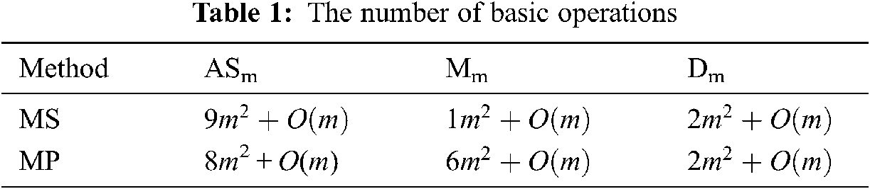
Figs. 5–6, graphically illustrates these percentage ratios. It is evident from Figs. 5–6 that MS method has dominating efficiency as compared to MP method.

4  Numerical Results

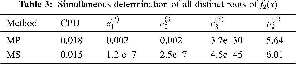
Here, we compare numerical results of our newly constructed method MS with Petković et al. method MP of convergence order 6. All numerical computations are performed using CAS Maple 18 with 64 digits floating point arithmetic with stopping criteria as follows.

where ek represents the absolute error. Take ε = 10−30 as tolerance for simultaneous methods. In all Tables stopping criteria (i) is used, CPU represents computational time in seconds and ρk(i) represents local computational order of convergence [23].

Applications in Engineering

In this section, we discuss some applications in engineering.

Example 1: [24] Blood Rheology Model

Blood, which is a non-Newtonian fluid is modeled as a Caisson Fluid. Caisson fluid model predicts that simple fluid like water, blood will flow through a tube in such a way that the central core of the fluids will move as a plug with little deformation and velocity gradient occurs near the wall.

To elaborate the plug flow of Caisson fluid flow, we used the following non-linear equation:

G=1−167x+43x−121x4, (28)

where reduction in flow rate is measured by G. Using G = 0.40 in Eq. (28), we have:

f1(x)=1441x8−863x5−0.05714285714x4+169x2−3.624489796x+0.36 (29)

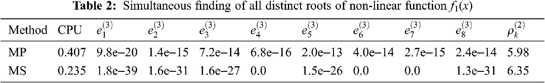
The exact solutions of Eq. (29) are graphed using maple command smartplot3d [f1(x)], shown in Fig. 7.

The exact roots of Eq. (29) up to ten decimal place are:

and

are chosen as initial guessed values. Tab. 2, clearly shows the dominance behavior of MS over MP iterative method in terms of CPU time and absolute error. Roots of f1(x) are calculated at third iteration.

Example 2: [25] Fluid Permeability in Biogels

Specific Hydraulic Permeability relates the pressure gradient to fluid velocity in porous medium (agarose gel or extracellular Fiber matrix) results the following non-linear polynomial equation:

k=Rex320(1−x)2, (30)

or Rex3−20k(1−x)2=0 (31)

where k is specific hydraulic permeability, Re radius of the fiber and 0 ≤ x ≤ 1 is the porosity.

Using k = 0.4655 and Re = 100*10−9, we have:

f2(x)=−100∗10−9x3+9.3100∗x2−18.6200∗x+9.3100 (32)

The exact solution are 3D-plot for different values of Re and k are graphed using maple command smartplot3d [f2(x) and f3(x)] shown in Fig. 8 for f2(x) and Fig. 9 for f3(x) respectively. Fig. 10, shows combined graph of f2(x) and f3(x) for − 5 ≤ k ≤ 5,  − 5 ≤ Re ≤ 5,  − 400 ≤ x ≤ 400.

The exact roots of Eq. (32) are

ζ1 = 0.9999999997,  ζ2 = 1.000000000,   ζ3 = 9.31*1018. The locations of exact root of Eq. (31) on x-axis as shown in Fig. 1.

We choose the following initial estimates for simultaneous determination of all roots of Eq. (32):

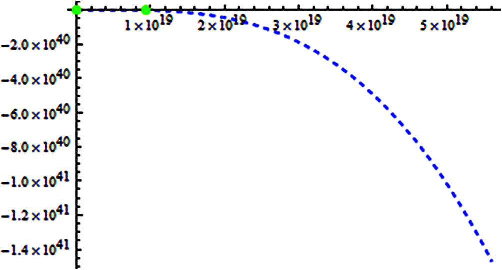
Figure 1: Shows location of exact real roots of f2(x) on x-axis

Using k = 0.3655 and Re = 10*10−9, we have:

f3(x)=−100∗10−9x3+9.3100∗x2−18.6200∗x+7.3100 (33)

The exact roots of Eq. (33) are

ζ1 = 0.9999999997,  ζ2 = 1.000000000,  ζ3 = 7.31*1018. The locations of exact root of Eq. (33) on x-axis are shown in Fig. 2.

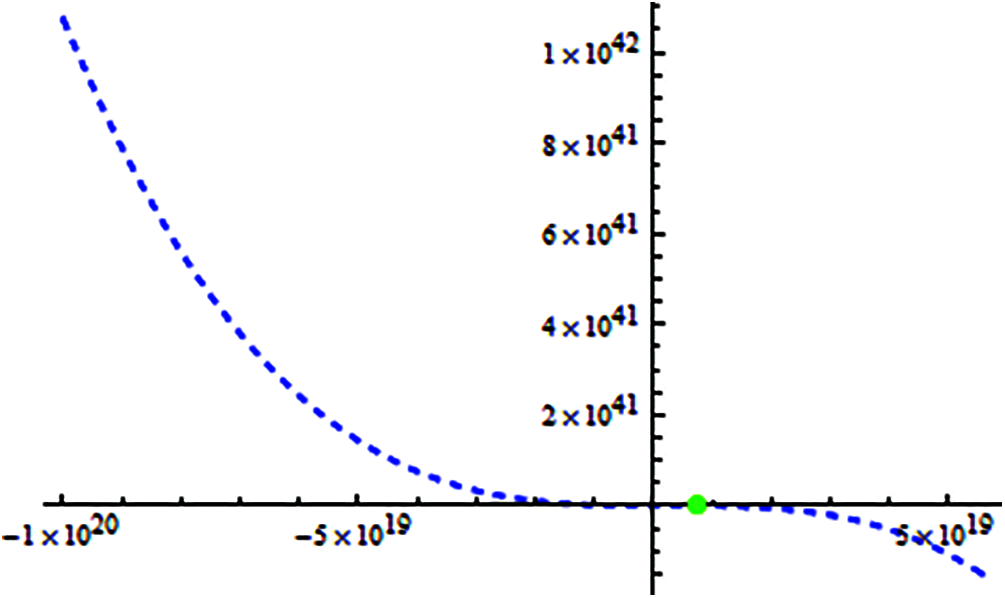
Figure 2: Shows location of exact real roots of f3(x) on x-axis

We choose the following initial estimates for simultaneous determination of all roots of Eq. (33):

Tab. 3, clearly shows the dominance behavior of MS over MP iterative method in terms of CPU time and absolute error. Roots of f2(x) are calculated at third iteration.

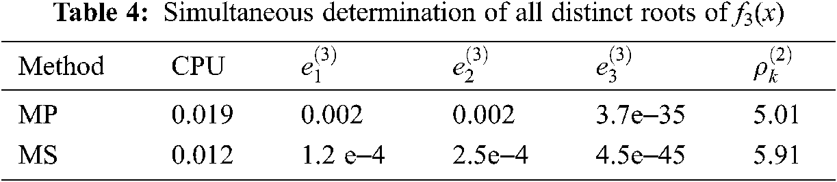
Tab. 4, clearly shows the dominance behavior of MS over MP iterative method in terms of CPU time and absolute error. Roots of f3(x) are calculated at the third iteration. Figs. 7–10, shows analytical approximate solution of f1(x) − f3(x) using maple command smartplot3d. Figs. 1–10, clearly show that analytical approximate and exact solutions match.

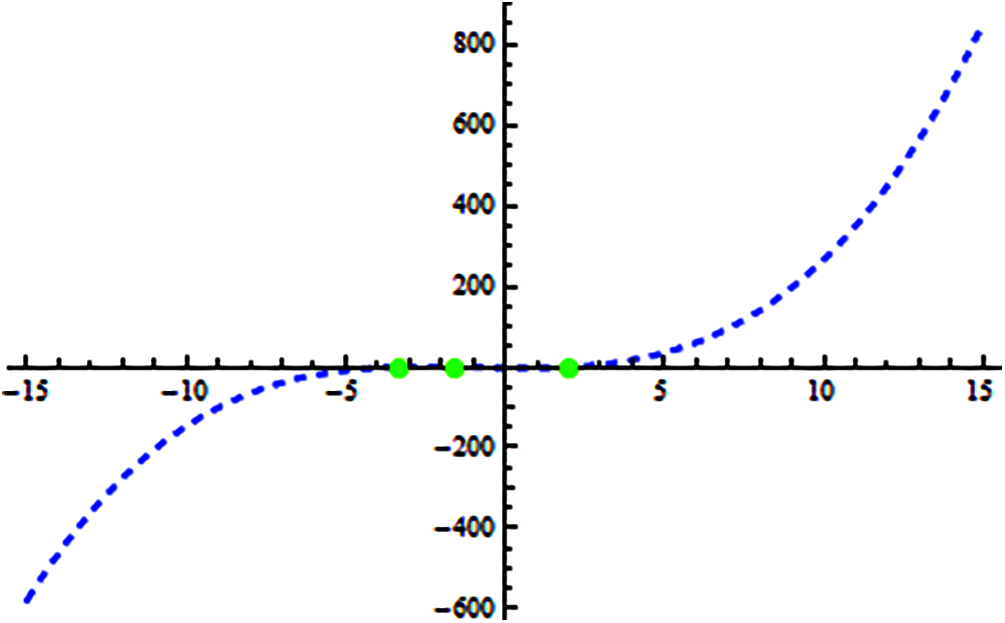
Figure 3: Shows location of exact real roots of f4(x) on x-axis

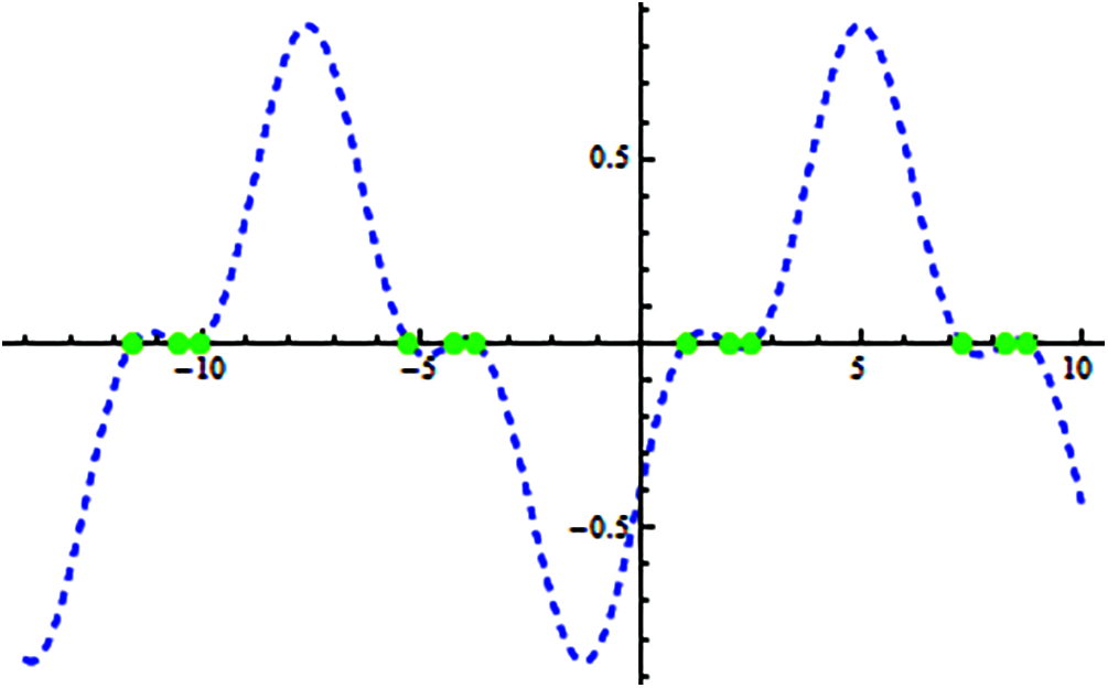
Figure 4: Shows location of exact real roots of f5(x) on x-axis

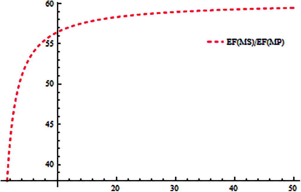
Figure 5: Shows computational efficiency of methods MS w.r.t method MP

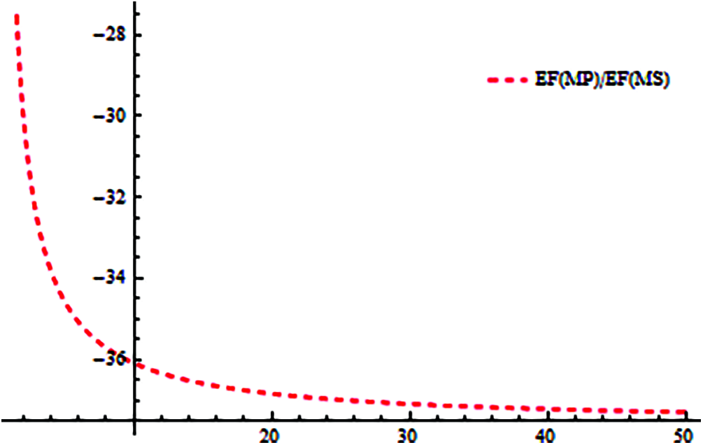
Figure 6: Shows computational efficiency of methods MP w.r.t method MS

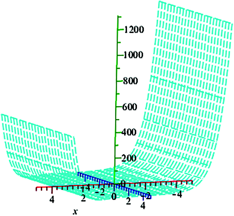
Figure 7: Shows the analytical solution of f1(x) graphically

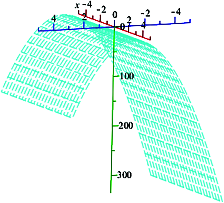
Figure 8: Shows graphically the analytical solution of f2(x) using maple command “smartplot3d [f2(x)] for k =0.4655, Re=100

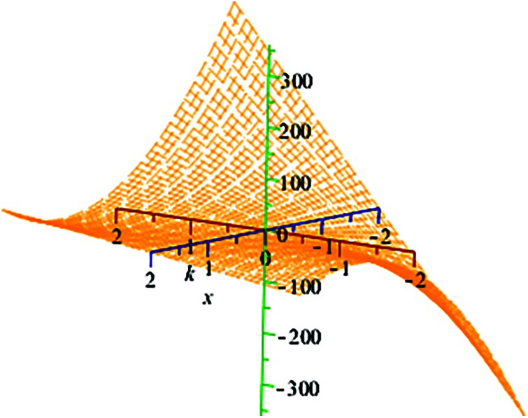
Figure 9: Shows the analytical solution of f3(x) in maple using command “smartplot3d [f3(x)]” for −5≤k≤5,Re=10

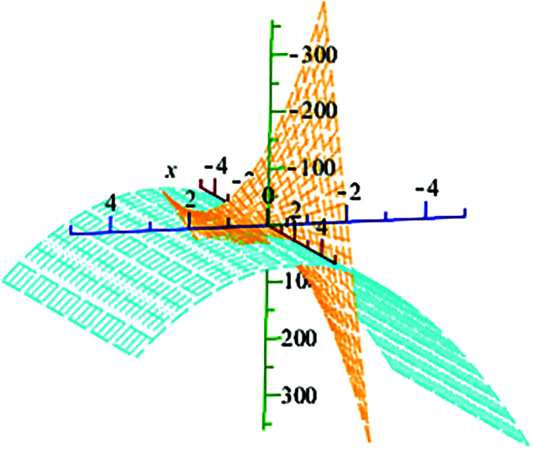
Figure 10: Shows graphically the analytical solution of f1(x) using maple command “smartplot3d [f2(x) or f3(x)].” for − 5 ≤ k ≤ 5, − 400 ≤ x ≤ 400

Example 3: [26] Beam Designing Model (An Engineering Problem)

An engineer considers a problem of embedment x of a sheet-pile wall resulting a non-linear function given as:

f4(x)=x3+2.87x2−10.284.62−x. (34)

The exact roots of Eq. (34) are represented in Fig. 3 on x-axis and ζ1 = 2.0021,  ζ2 = −3.3304,  ζ3 = −1.5417. The initial guessed values are taken as:

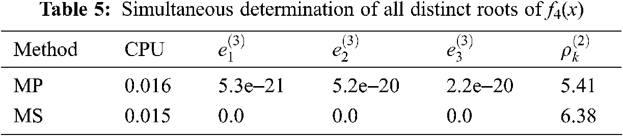
Tab. 5, clearly shows the dominance behavior of MS over MP iterative method in terms of CPU time and absolute error. Roots of f4(x) are calculated at the third iteration.

Example 4: [27]

Consider

f5(x)=sin3⁡(x−12)sin3⁡(x−22)sin3⁡(x−2.52), (35)

with multiple exact roots of Eq. (35) as represented in Fig. 4 are ζ1 = 1, ζ2 = 2, ζ3 = 2.5. The initial guessed values of the exact roots have been taken as:

For distinct roots, we have:

f5−1∗(x)=sin⁡(x−12)sin⁡(x−22)sin⁡(x−2.52). (36)

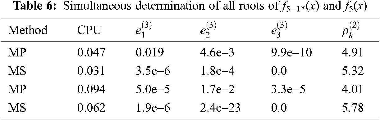
Tab. 6, clearly shows the dominance behavior of MS over MP iterative method in terms of CPU time and absolute error. Roots of f5−1*(x) and f5(x) are calculated at the third iteration.

5  Conclusion

In this research article, we developed an optimal family of single root finding method of convergence order 4 and then extended this family to an efficient numerical algorithm of convergence order 6 for approximating all roots of Eq. (1). The computational efficiency of our method MS is very large as compared to MP as given in Tab. 1, which is also obvious from Figs. 5–6. From all Figs. 1–10, Tabs. 1–6, residual error and CPU time clearly show the dominance efficiency of iterative scheme MS as compared to MP on same number of iterations.

Funding Statement: The authors received no specific funding for this study.

Conflicts of Interest: The authors declare that they have no conflicts of interest to report regarding the present study.

References

 1.  M. Cosnard and P. Fraigniaud, “Finding the roots of a polynomial on an MIMD multicomputer,” Parallel Computing, vol. 15, no. 1–3, pp. 75–85, 1990. [Google Scholar]

 2.  A. Naseem, M. A. Rehman, T. Abdeljawad and Y. M. Chu, “Novel iteration schemes for computing zeros of non-linear equation with engineering applications and their dynamics,” IEEE Access, vol. 9, pp. 92246–92262, 2021. [Google Scholar]

 3.  J. R. Sharma and H. Arora, “A new family of optimal eight order methods with dynamics for non-linear equations,” Applied Mathematics and Computation, vol. 273, pp. 924–933, 2016. [Google Scholar]

 4.  A. Naseem, M. A. Rehman and T. Abdeljawad, “Numerical methods with engineering applications and their visual via polynomiography,” IEEE Access, vol. 9, pp. 99287–99298, 2021. [Google Scholar]

 5.  S. A. Sariman and I. Hashim, “New optimal newton-householder methods for solving nonlinear equations and their dynamics,” Computer, Material & Continua, vol. 65, no. 1, pp. 69–85, 2020. [Google Scholar]

 6.  A. Naseem, M. A. Rehman and T. Abdeljawad, “Numerical algorithms for finding zeros of nonlinear equations and their dynamical aspects,” Journal of Mathematics, vol. 2011, pp. 1–11, 2020. [Google Scholar]

 7.  A. Naseem, M. A. Rehman and T. Abdeljawad, “Some new iterative algorithms for solving one-dimensional non-linear equations and their graphical representation,” IEEE Access, vol. 9, pp. 8615–8624, 2021. [Google Scholar]

 8.  S. Kanno, N. Kjurkchiev and T. Yamamoto, “On some methods for the simultaneous determination of polynomial zeros,” Japan Journal of Applied Mathematics, vol. 13, pp. 267–288, 1995. [Google Scholar]

 9.  O. Albert, “Iteration methods for finding all zeros of a polynomial simultaneously,” Mathematics of Computation, vol. 27, no. 122, pp. 339–334, 1973. [Google Scholar]

10. P. D. Proinov and S. I. Cholakov, “Semi local convergence of chebyshev-like root-finding method for simultaneous approximation of polynomial zeros,” Applied Mathematics and Computation, vol. 236, no. 1, pp. 669–682, 2014. [Google Scholar]

11. B. Sendov, A. Andereev and N. Kjurkchiev, “Numerical solutions of polynomial equations,” In: P. G. Ciarlet, J. L. Lions (Eds.Handbook of Numerical Analysis, Elsevier Science, New York, vol. III, pp. 629–777, 1994. [Google Scholar]

12. T. F. Li, D. S. Li, Z. D. Xu and Y. I. Fang, “New iterative methods for non-linear equations,” Applied Mathematics and Computations, vol. 197, no. 2, pp. 755–759, 2008. [Google Scholar]

13. N. A. Mir, R. Muneer and I. Jabeen, “Some families of two-step simultaneous methods for determining zeros of non-linear equations,” ISRN Applied Mathematics, vol. 2011, pp. 1–11, 2011. [Google Scholar]

14. P. D. Proinov and M. T. Vasileva, “On the convergence of higher-order ehrlich-type iterative methods for approximating all zeros of polynomial simultaneously,” Journal of Inequalities and Applications, vol. 336, pp. 1–26, 2015. [Google Scholar]

15. M. Shams, N. Rafiq, N. A. Mir, B. Ahmad, S. Abbasi et al., “On computer implementation for comparison of inverse numerical schemes,” Computer System Science and Engineering, vol. 36, no. 3, pp. 493–507, 2021. [Google Scholar]

16. W. M. Nourein, “An improvement on two iteration methods for simultaneously determination of the zeros of a polynomial,” International Journal of Computational Mathematics, vol. 6, pp. 241–252, 1977. [Google Scholar]

17. G. H. Nedzhibov, “Iterative methods for simultaneous computing arbitrary number of multiple zeros of nonlinear equations,” International Journal of Computer Mathematics, vol. 90, no. 5, pp. 994–1007, 2013. [Google Scholar]

18. A. R. Alharbi, M. I. Faisal, F. A. Shah, M. Waseem, R. Ullah et al., “Higher order numerical approaches for nonlinear equations by decomposition technique,” IEEE Access, vol. 7, pp. 44329–44337, 2019. [Google Scholar]

19. H. T. Kung and J. F. Traub, “Optimal order of one-point and multipoint iteration,” Journal of the ACM, vol. 21, no. 4, pp. 643–651, 1974. [Google Scholar]

20. N. A. Mir, N. Yasmin and N. Rafiq, “Quadrature based two-step iterative methods for nonlinear equations,” General Mathematics, vol. 16, no. 1, pp. 33–45, 2008. [Google Scholar]

21. S. M. Ilic and L. Rancic, “On the fourth order zero-finding methods for polynomials,” Filomat, vol. 17, pp. 35–46, 2003. [Google Scholar]

22. M. S. Petkovic, L. D. Petkovic and J. Dμzunic, “On an efficient method for simultaneous approximation of polynomial multiple roots,” Applicable Analysis and Discrete Mathematics, vol. 8, pp. 73–94, 2014. [Google Scholar]

23. N. Rafiq, S. Akram, M. Shams and N. A. Mir, “Computer geometries for finding all real zeros of polynomial equations simultaneously,” Computer Material and Continua, vol. 69, no. 2, pp. 2636–2651, 2021. [Google Scholar]

24. R. L. Fournier, “Basic transport phenomena in biomedical engineering,” New York: Taylor & Francis, pp. 1–611, 2007. [Google Scholar]

25. W. M. Saltzman, “Drug delivery: Engineering principal for drug therapy,” New York: Oxford University Press 2001. [Google Scholar]

26. M. Shams, N. A. Mir, N. Rafiq, A. O. Almatroud and S. Akram, “On dynamics of iterative techniques for nonlinear equation with application in engineering,” Mathematical Problems in Engineering, vol. 2020, pp. 1–17, 2020. [Google Scholar]

27. M. R. Farmer, “Computing the zeros of polynomials using the divide and conquer approach,” Ph.D. dissertation, Department of Computer Science and Information Systems, Birkbeck, University of London, 2014. [Google Scholar]

This work is licensed under a Creative Commons Attribution 4.0 International License, which permits unrestricted use, distribution, and reproduction in any medium, provided the original work is properly cited.