Computer Systems Science & Engineering DOI:10.32604/csse.2022.022152
Article

Towards Improving Predictive Statistical Learning Model Accuracy by Enhancing Learning Technique

Ali Algarni1, Mahmoud Ragab2,3,4,*, Wardah Alamri5 and Samih M. Mostafa6

1Statistics Department, Faculty of Science, King Abdulaziz University, Jeddah, 21589, Saudi Arabia
2Information Technology Department, Faculty of Computing and Information Technology, King Abdulaziz University, Jeddah, 21589, Saudi Arabia
3Mathematics Department, Faculty of Science, Al-Azhar University, Naser City, 11884, Egypt
4Centre of Artificial Intelligence for Precision Medicines, King Abdulaziz University, Jeddah, 21589, Saudi Arabia
5Educational Technology Department, Educational Graduate Studies Faculty, King Abdulaziz University, Jeddah, 21589, Saudi Arabia
6Computer Science Department, Faculty of Computers and Information, South Valley University, Qena, 83523, Egypt
*Corresponding Author: Mahmoud Ragab. Email: mragab@kau.edu.sa
Received: 29 July 2021; Accepted: 30 August 2021

Abstract: The accuracy of the statistical learning model depends on the learning technique used which in turn depends on the dataset’s values. In most research studies, the existence of missing values (MVs) is a vital problem. In addition, any dataset with MVs cannot be used for further analysis or with any data driven tool especially when the percentage of MVs are high. In this paper, the authors propose a novel algorithm for dealing with MVs depending on the feature selection (FS) of similarity classifier with fuzzy entropy measure. The proposed algorithm imputes MVs in cumulative order. The candidate feature to be manipulated is selected using similarity classifier with Parkash’s fuzzy entropy measure. The predictive model to predict MVs within the candidate feature is the Bayesian Ridge Regression (BRR) technique. Furthermore, any imputed features will be incorporated within the BRR equation to impute the MVs in the next chosen incomplete feature. The proposed algorithm was compared against some practical state-of-the-art imputation methods by conducting an experiment on four medical datasets which were gathered from several databases repository with MVs generated from the three missingness mechanisms. The evaluation metrics of mean absolute error (MAE), root mean square error (RMSE) and coefficient of determination (R2 score) were used to measure the performance. The results exhibited that performance vary depending on the size of the dataset, amount of MVs and the missingness mechanism type. Moreover, compared to other methods, the results showed that the proposed method gives better accuracy and less error in most cases.

Keywords: Bayesian ridge regression; fuzzy entropy measure; feature selection; imputation; missing values; missingness mechanisms; similarity classifier; medical dataset

1  Introduction

MVs are considered a critical problem that can occur in many scientific areas such as biological, psychological, or medical [1]. Commonly, many reasons may lead to the occurrence of MVs, for instance, wrong data entry, improper data collection, management of similar but not identical datasets and malfunctioning measurement equipment [2]. Machine learning (ML), big data and any data driven tool require high data quality which results in good analysis and outcomes. The existence of MVs within a dataset can result in problems, for instance, bad data analysis, reducing the research results obtained from such dataset and presenting amount of bias [3]. To this end, significant information is incorporated within MVs which should be manipulated before using the incomplete dataset with any data driven tool. Furthermore, many researches were done and novel algorithms were proposed to solve the problem of MVs, especially in medical data [4]. Nevertheless, several imputation algorithms may result in poor imputation and may fail in handling all MVs in the dataset. In addition, they may not deal with all missingness mechanisms. These shortcomings of these algorithms encouraged the authors to propose a novel algorithm introduced in this paper. The proposed algorithm utilizes the most significant feature to impute MVs in cumulative order. Besides MVs, FS also affects the ML model performance.

1.1 Feature Selection

High dimensionality data is problematic especially in circumstances when a dataset contains a few numbers of training instances and a large number of features. This type of data commonly exists in medicine where cost and time problems may limit the number of training observations, while the number of diseases increases through the years [5]. FS helps to overcome the problem of high dimensionality by selecting a subset of features that have a strong relationship with the target feature. In addition, in the existence of MVs the FS is considered a vital preprocessing step such as correlation, mutual information and fuzzy FS. Dropping features that hold a large number of MVs (e.g., >50%) is an easy solution. But such a solution may result in bad analysis, losing the ability to recognize statistically significant variations and may also generates bias. Missingness mechanisms have a large effect on FS that’s why before applying any FS technique missingness mechanisms need to be taken into consideration [3].

1.2 Missingness Mechanisms

Before introducing different methods for handling MVs, it is essential to present the different types of missingness mechanisms (i.e., the reason for the occurrence of MVs in data). MVs are commonly classified to one of three MVs mechanisms [6]:

•   Missing Completely at Random (MCAR): This type of MVs mechanisms happens when the probability of the existence of MVs is independent from any other features in the data. From statistical perspective, MCAR can be stated as in Eq. (1) [1].

f(M|Y,∅)=f(M|Y) forallY,∅ (1)

where M and Y represent the missing and observed data respectively. The conditional probability is denoted by f and ∅ represents the unknown parameter. An example of MCAR MVs occur when the measuring equipment stops working correctly [7].

•   Missing at Random (MAR): In this mechanism the relationship between MVs and other features existed in the dataset is a dependent relationship. In other words, the probability of the occurrence of MVs depends on observed values in other features and not on other MVs in the target feature [8]. MAR can be represented as in Eq. (2) [1].

f(M|Y,∅)=f(M|Yobs,∅) forallYmis,∅ (2)

where Ymis and Yobs are the missing and observed values from Y respectively. From a medical perspective, this situation may occur when an experiment has not been accomplished because a feature within the dataset shows that the patient is a woman for example [7].

•   Missing Not at Random (MNAR): For this type, there is a dependent relationship between the MVs and the observed data. MNAR can be expressed using Eq. (3) [1].

f(M,Y|θ,∅)=f(Y|θ)f(M|Y,∅) (3)

where θ (i.e., parameter of the distribution Y ). is estimated from the detected data The distribution of the missingness is denoted by ∅. An example of MNAR MVs, when people having a too high or too low income reject to reveal it [7].

1.3 Handling Missing Data

The simplest methods for handling MVs are traditional methods. Traditional methods can be deletion (i.e., delete instances that hold MVs), mean or median (i.e., replace the MVs with the mean or median of the feature that holds MVs) substitution [9]. Deletion can be case deletion or pairwise deletion. Case deletion (a.k.a., listwise) in which any instance holds MVs is dropped from analysis. In many statistical packages listwise is the default choice [10]. Pairwise deletion is considered a selective method, which tries to minimize the lost amount of data instances that occur in case of using the listwise method by including into the analysis the instances with MVs. In other words, pairwise deletion will drop only particular features with MVs from the analysis and use the remainder features with no MVs. The selection of features varies from analysis to another depending on the missingness. Using deletion methods results in reducing the data size [11].

The other methods that overcome the defects of deletion methods are called imputation methods. In imputation methods, predefined (mean, median, etc.) or estimated (using statistical methods, ML algorithms, etc.) value is used instead of MVs [12]. Imputation is classified into single and multiple imputation. In single imputation, MVs are imputed by a value one time. Though, single imputation does not require computational resources it can result in biased results [3]. In multiple imputation, m copies from the original dataset are generated. In each generated dataset, MVs are imputed using single imputation techniques. The final imputed dataset is the average analysis of the m imputed datasets [13,14]. ML algorithms can also be used to predict MVs depending on using the available information within the given dataset. Some examples of ML techniques that are used to predict MVs include linear regression, k-nearest neighbour (KNN), decision trees [1] and BRR. BRR is the predictive model used within the proposed algorithm in this paper to predict MVs, which can be expressed using Eq. (4) [15].

y∼N(μ,α) (4)

where:

The target feature is denoted by y which is distributed as a normal distribution characterized by mean μ=βX and variance α . β={β0,β1,β2,…,βq} denotes the unknown parameters and X={x1,x2,…,xq} denotes the independent features. The number of independent features is represented by q . α and λ represent the regularization parameters which are assessed jointly while fitting the model through maximizing the log marginal likelihood and both of them are assumed to be distributed as gamma distribution. α1,α2,λ1,λ2 are hyper-parameters of the gamma prior distributions.

The rest of the paper is organized as follows: Section 2 presents a brief literature review about analysis of MVs. Sections 3 and 4 reveal the proposed algorithm and explains in detail the experimental setup, respectively. Section 5 is devoted to the presentation of the results and discussion while section 6 concludes this paper and exhibits some perspectives of future work.

2  Literature Review

Hot-Deck (HD) imputation is a popular choice for manipulating MVs in survey research. Hot deck technique finds a similar dataset and imputes MVs by substituting MVs with an observed value from this dataset. Although, this technique is easy to implement but it may be computationally [16]. The method that looks like hot-deck imputation but the data source and current data set must be different from each other is known as Cold-Deck imputation [17]. In many time-series and longitudinal data, one of the most common and used imputation methods is the Last Observation Carried Forward (LOCF). This method imputes each missing value using the last observed value from the same data [18]. The maximum likelihood method can also be used to manipulate MVs. The maximum likelihood assumes that the detected data is a sample taken from a multivariate normal distribution. After the estimation of the parameters using the available information, the MVs are imputed depending on the estimated parameters [19,20]. In regression imputation, the complete features are used to predict the MVs within the features that contain MVs. The predicted values is used to impute the MVs. Regression imputation keeps all data and hence overcomes the pairwise or listwise deletion and does not change the shape of the distribution. In regression imputation, no information is changed or added and the standard error is reduced, hence, little or no biased predictions are generated from the imputation stage [21]. Expectation-Maximization Imputation (EMI) is a kind of the maximum likelihood technique that can be used to manipulate MVs. EMI uses the values assessed by the use of maximum likelihood methods to impute MVs [22]. This method begins with the expectation step, through which the parameters (e.g., means, covariances, and variances) are assessed, possibly by the use of listwise deletion. Predicting MVs is implemented after creation of a regression equation by the use of the estimated parameters. In the maximization step, the regression equations are used to impute MVs. By repeating the expectation and maximization steps until the covariance matrix for the successive iteration is almost the same as that for the previous one. When there is large amount of MVs, EMI method require long time to converge. EMI can result in biased parameter assessments, hence, the standard error is underestimated [21]. KNN imputation technique is considered as one of the most commonly used imputation techniques KNN detects between the complete instances the k most nearest neighbors of a missing data point. The MVs are then imputed with an average of the values of its neighbors in this point. The performance of KNN is extremely bounded especially when the percentage of MVs is high. A simple improvement for manipulating MVs using KNN lies in looking for incomplete neighbors (i.e., act as donors) of an instance given that these neighbors are detected for the features missing instances. This method is known as incomplete case k-nearest neighbors imputation (ICkNNI). ICkNNI in somewhat considered a complex method [23]. Methods that manipulate MVs problems directly without the need of any deletion or imputation step have been developed. For example, logistic regression with MVs by using a Gaussian mixture model to assess the conditional density functions was performed by the authors in [24]. For clustering purposes, the Kernel Spectral Clustering (KSC) algorithm was proposed, which encodes as a set of supplemental soft constraints the partially detected features [25]. MLPimpute is a novel algorithm for handling MVs depending multilayer perceptron (MLP) networks was proposed. Although MLP exhibits a good accuracy the relationship between data genes is not sufficient for the method [26]. An iterative learning method consists of fuzzy k-means and decision trees was used to manipulate MVs. When this iterative learning compared with KNNimpute it exhibits a better accuracy [27].

3  Proposed Algorithm

This section aims to introduce and elaborate the proposed algorithm in details. The next procedural steps help in clarifying the proposed algorithm.

•   Splitting Dataset: The proposed algorithm gets a dataset D as input which incorporates MVs, then creates from D two subsets. The first set X(comp) holds all features with no MVs and the second set X(mis) holds all features with MVs. The target feature was assumed to be perfect feature (i.e., does not hold MVs), thus X(comp) holds all perfect features besides the target feature y .

•   Feature Selection: The proposed algorithm uses the FS of fuzzy entropy measure introduced by Parkash et al. given by Eq. (5) with the similarity-based classification [28]

S⟨x,v⟩=(1t∑r=1twr(1−|x(fr)p−v(fr)p|)mp)1m,x,vϵ[0,1]t (5)

where t represents the number of features of varied types f1,...,ft that can be observed from the objects, the ideal vector vi=(vi(f1),...,vi(ft)) should be determined for every class i . x=(x(f1),...,x(ft)) represents vectors which belong to known class. m is the power value that is obtained from the generalized mean from the generalized Lukasiewicz structure. The parameter p can be detected from the generalized Lukasiewicz structure. wr is a weight parameter. The weights were set as one.

H(A;w)=∑j=1n(sinπμA(xj)2+sinπ(1−μA(xj))2−1) (6)

where H represents the fuzzy entropy. j represents the number of features and the fuzzy values are denoted by μA(xj) . A denotes the fuzzy set which is the maximum element of the ordering specified by H when μA(x) = 0.5.

The proposed algorithm chooses the feature that exhibits the lowest fuzzy entropy, which gives a strong relationship with the output feature.

•   Imputation: After the candidate feature Xg(miss) is being selected, the model is fitted using X(comp) as the input features and the candidate feature as target with the cumulative formula described in Eq. (7).

Xg(miss)∼N(μg,αg) (7)

where:

where g=1,2,…,m. m is the number of features holding MVs and c is the number of perfect features.

•   Update datasets: The selected feature dropped from X(mis) and after imputing MVs within the Xg(miss) , the imputed feature Ximp(mis) is added to X(comp) . Now X(comp) holds all perfect features, Ximp(mis) and y . A new Xg(miss) from X(mis) is chosen. The model is fitted with the cumulative formula with X(comp) as an input features and the new Xg(miss) as the target feature.

Repeat from step 2 of feature selection until X(mis) holds no features, at that moment return ( X(comp) ) as the imputed dataset as described in the following algorithm.

4  Experimental Setup

4.1 Datasets

Usually, applying and comparing several imputation algorithms on diverse datasets versus the proposed algorithm will result in different imputation performances. Furthermore, this difference in imputation helps in judgement about the compared algorithms and the proposed one and also gives an insight about how the proposed algorithm will perform in future and in different situations. The focus in this paper is on medical datasets. The used datasets in this experiment were obtained from several data repositories and are freely access. Tab. 1 gives an overview about the specifications of the datasets used in the experiment. In each dataset, the generation of MVs proportions, 10%, 20%, 30%, 40% and 50%, were performed using the ampute function from the R environment [29] for every missingness mechanism, MAR, MCAR and MNAR.

Five practical imputation algorithms were used in the experiment against the proposed algorithm. Tab. 2 describes briefly the compared algorithms used in the experiment.

The experiments were conducted using a laptop with the following specification: Windows 10 OS, 4 GB memory, AMD A4-6210 APU with AMD Radeon R3 Graphics (1.80 GHz) processor, 500 GB HDD and Python (version 3.7) programming language and R (version 3.5.2).

4.2 Evaluation Metrics

Imputation performance can be measured using various metrics. This section exhibits an overview of most metrics used in the experimental implementation to measure the imputation performance; these metrics include MAE, RMSE, and R2 score.

4.2.1 MAE and RMSE

MAE is used to calculate the average of the absolute differences between the predicted and true values. It gives an intuition about the magnitudes (absolute values) of the error in prediction, but does not offer any idea about the direction of the prediction (i.e., under or over predicting) [36]. RMSE is much like the MAE in that it gives an idea of the magnitude of error. Furthermore, as the variance related to the error magnitudes distribution increases RMSE also increases and MAE is steady. Eqs. (8) and (9) describes MAE and RMSE respectively [3]

MAE=1n∑l=1n|yl−yl^| (8)

RMSE=1n∑l=1n(yl−yl^)2 (9)

where the real and predicted values are denoted as yl and yl^ of the lth observation respectively and the number of the observations is denoted as n .

4.2.2 R2 Score

R2 score, given by Eq. (10), gives an indication of the prediction’s goodness of fit to the true values. From a statistical perspective, the R2 score has been dubbed as the coefficient of determination [14].

R2(y,y^)=1−∑i=1n(yl−yi^)2∑l=1n(yl−y¯)2 (10)

where:

y¯ represents the mean of the detected data.

5  Results and Discussion

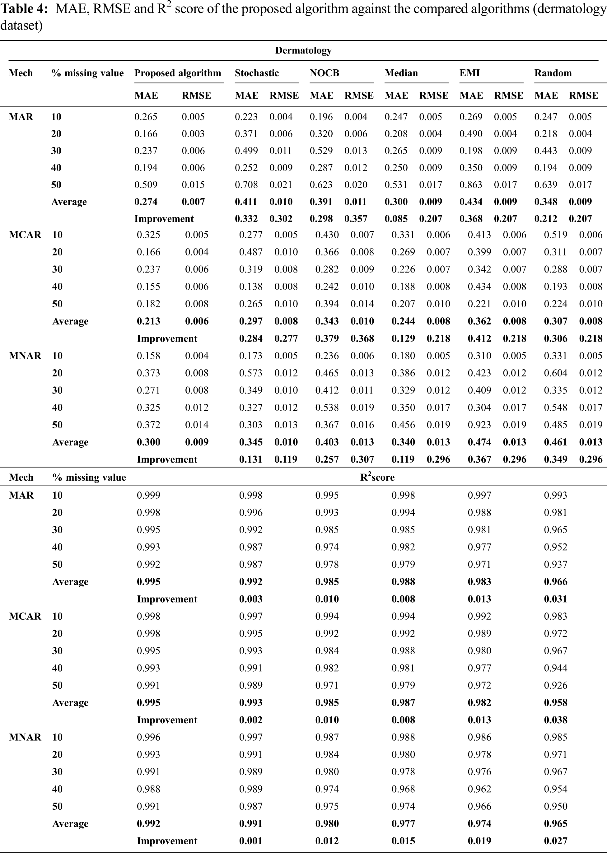
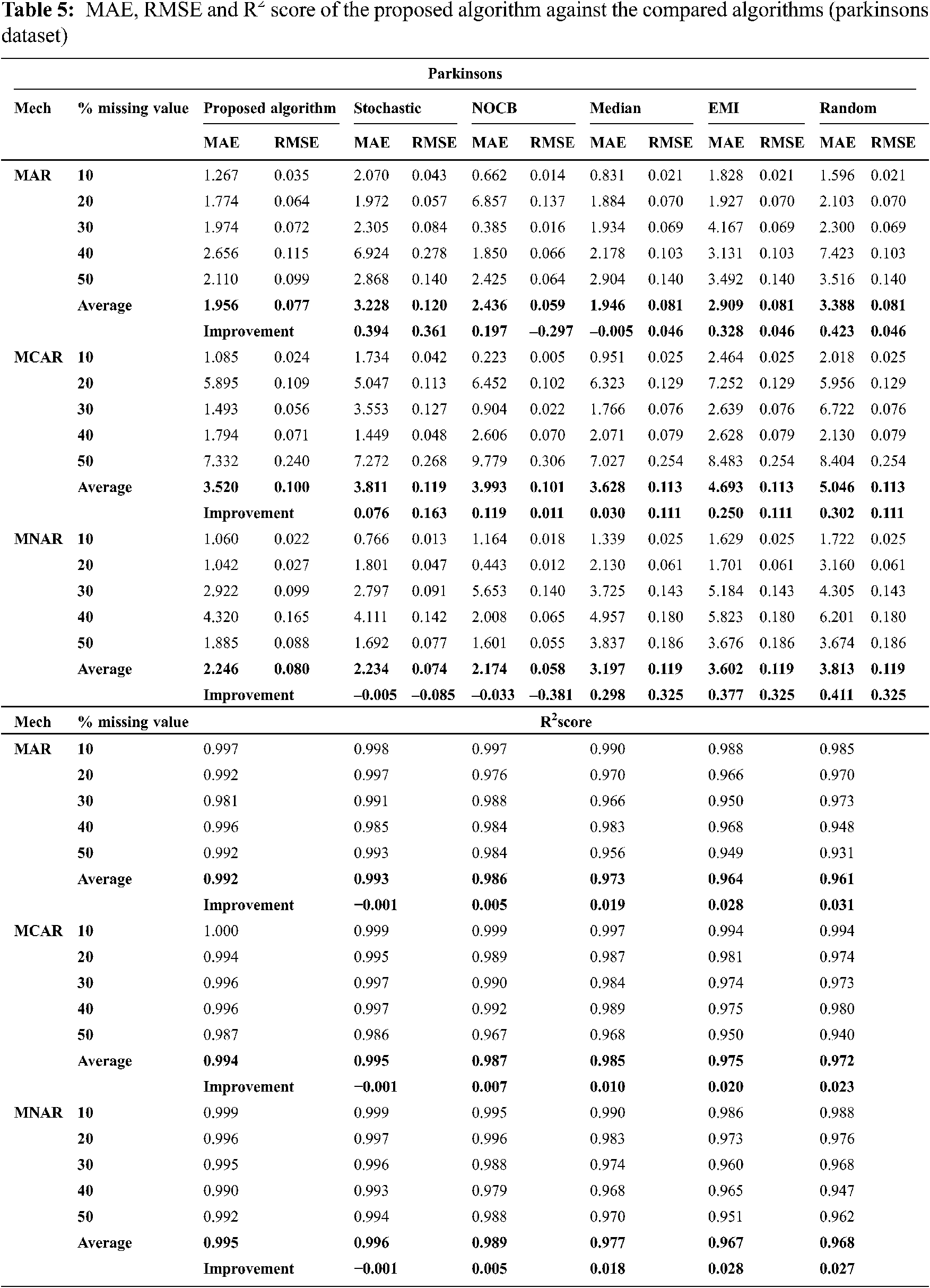
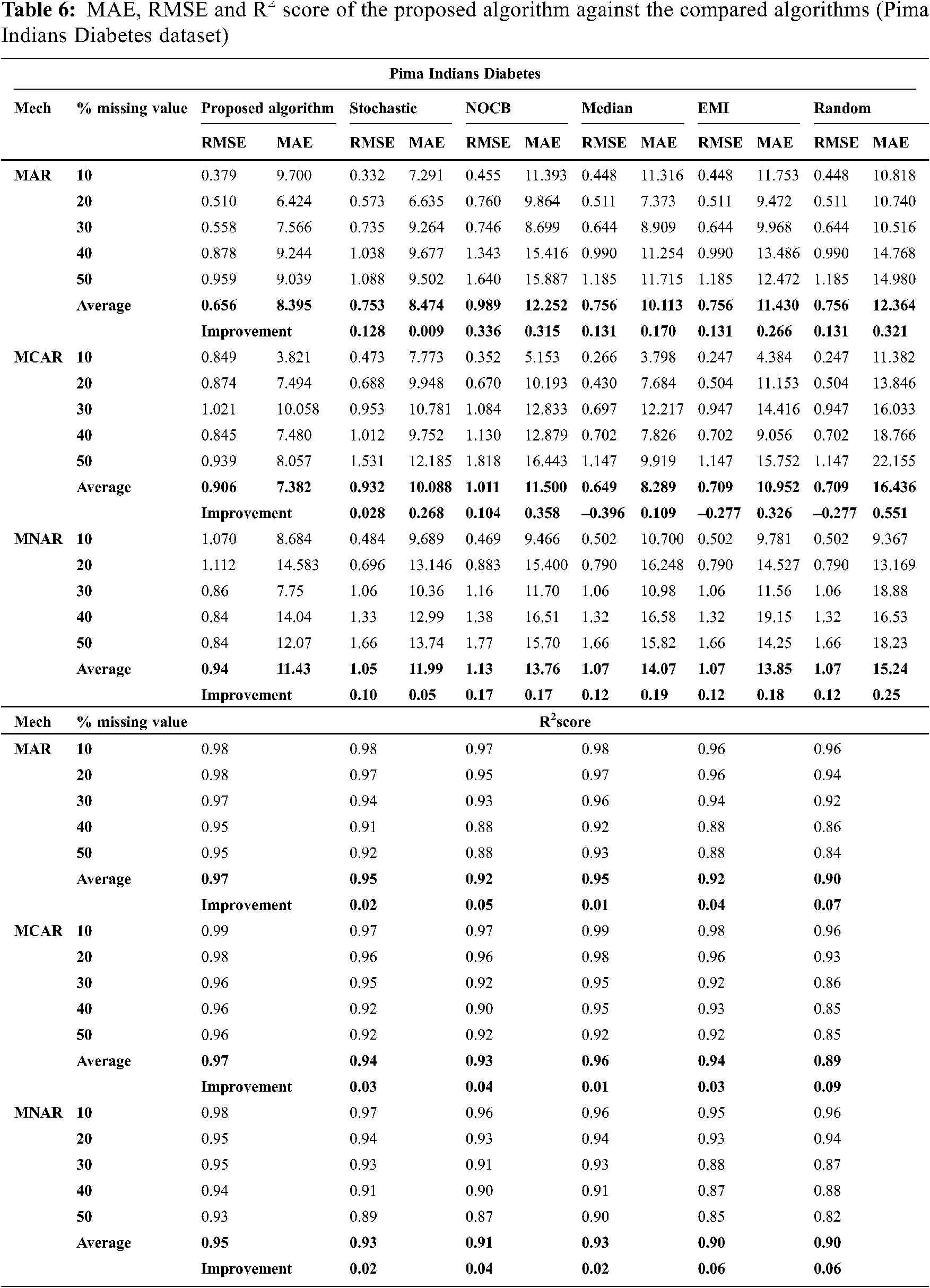
Figs. 1 to 3 present the improvement in performance, using RMSE, MAE and R2 score, of the compared algorithms versus the proposed one. The performance evaluation of the proposed algorithm against the compared algorithms for each MVs percentage, 10%, 20%, 30%, 40% and 50%, generated from the missingness mechanisms, MAR, MCAR and MNAR, is presented in more details in Tabs. 3 to 6. The results exhibit that the performance differs from one algorithm to another depending on the dimension of the dataset, the missingness mechanism type, and the amount of MVs in the dataset. The computational complexity of both CBRL and CBRC is O(n).

This section is subdivided into two subsections. The first section explains the accuracy analysis evaluated using R2 score (higher values is better) and the second represents the error analysis evaluated using RMSE and MAE metrics (lower value is better).

5.1 Accuracy Analysis

This subsection exhibits that the proposed algorithm offers better accuracy versus the compared algorithms in many cases. The accuracy analysis is represented by calculating R2 score. Fig. 1 exhibits the improvement percentage of R2 score which is given by Eq. (10) for the proposed algorithm versus the compared algorithms. In what follows, the comparison of R2 score is discussed in detail. In all missigness mechanisms, R2 score of the proposed algorithm is better than nocb, median, EMI and random when applied on all datasets used in the experiment. In addition, R2 score of the proposed algorithm is better than stochastic when applied on all used datasets but worse than stochastic when applied on parkinsons dataset in all missigness mechanisms.

5.2 Error Analysis

This subsection exhibits that the proposed algorithm gives lower error versus the compared algorithms in many cases. MAE and RMSE, given by Eqs. (8) and (9) respectively, are the metrics used for assessing the error in imputation. Figs. 2 and 3 exhibit the improvement percentage in evaluating both MAE and RMSE respectively.

In all missigness mechanisms, MAE given by the proposed algorithm is lower than MAE given by EMI and random when applied on all datasets used in the experiment. When the proposed algorithm is compared with stochastic in MAR and MCAR, it was observed that MAE granted by the proposed algorithm is the lowest in all used datasets. In MNAR, MAE of the proposed algorithm is better than stochastic in all used datasets except when applied on the parkinsons dataset. In MAR and MCAR, MAE of the proposed algorithm is better than nocb in all used datasets except when applied on the breast cancer dataset. In MNAR, MAE of the proposed algorithm is better than nocb in all used datasets except when applied on the breast cancer and parkinsons datasets. When the proposed algorithm is compared with median in MCAR it was observed that MAE of the proposed algorithm is better in all used datasets. In MAR, MAE of the proposed algorithm is better than median in all used datasets except when applied on the parkinsons dataset. In MNAR, MAE of the proposed algorithm is better than median in all used datasets except when applied on the breast cancer dataset.

In MAR and MCAR, RMSE of the proposed algorithm is better than stochastic in all used datasets. Also in MNAR, RMSE of the proposed algorithm is better than stochastic in all used datasets except when applied on the parkinsons dataset. When the proposed algorithm is compared with nocb in MAR and MNAR, it was noticed that RMSE of the proposed algorithm is better than nocb in all used datasets except when applied on the parkinsons and breast cancer datasets. When the proposed algorithm is compared with median, EMI and random in MAR and MNAR, it was observed that RMSE of the proposed algorithm is better in all used datasets. Also in MCAR, RMSE of the proposed algorithm is better than RMSE of median, EMI and random when applied in all datasets used in the experiment except in Pima Indians Diabetes and breast cancer datasets.

Figure 1: R2 score improvement percentage of the proposed algorithm versus the compared algorithms

Figure 2: MAE improvement percentage of the proposed algorithm versus the compared algorithms

Figure 3: RMSE improvement percentage of the proposed algorithm versus the compared algorithms

6  Conclusion

MVs are considered a critical problem in pattern recognition, ML and data mining applications. Many extensive studies have been performed for manipulating the problem of MVs especially in medical data. In addition to MVs, FS is the data preprocessing strategy which has been considered to be efficient when preparing data (specifically large volume data) in ML. It has been confirmed to be efficient and effective in handling high-dimensional data for any data dependent tool. Reducing the computational cost of modeling and the number of input features helps in improving the performance of the model.

In this paper, novel algorithm was proposed to manipulate MVs. The proposed algorithm depends on FS of similarity classifier with Parkash’s fuzzy entropy measure to select the candidate feature and the BRR model to predict MVs in the selected feature. Hence, the proposed algorithm consists mainly of two phases. In the first phase, the FS of similarity classifier with Parkash’s fuzzy entropy is used to select features to be imputed one after one. In the second phase, the MVs in the selected feature are predicted using the BRR model. The first and second phases are repeated until the imputation of the whole dataset. The proposed algorithm is easy to implement and can deal with all MVs from any missingness mechanism. Furthermore, the proposed algorithm exhibits a good performance against the compared algorithms.

In future research, the proposed algorithm will be implemented on new medical datasets like pulmonary embolism data and cardiovascular disease. Furthermore, additional performance metrics will be taken into consideration such as the normalized root mean square error (NRMSE), statistical tests and predictive accuracy (PAC).

Acknowledgement: This project was funded by the Deanship of Scientific Research (DSR) at King Abdulaziz University (KAU), Jeddah, Saudi Arabia, under grant No. (PH: 13-130-1442). The authors, therefore acknowledge with thanks DSR for technical and financial support.

Funding Statement: This project was funded by the Deanship of Scientific Research (DSR) at King Abdulaziz University (KAU), Jeddah, Saudi Arabia, under grant No. (PH: 13-130-1442).

Conflicts of Interest: The authors declare that they have no conflicts of interest to report regarding the present study.

References

 1.  M. S. Osman, A. M. Abu-Mahfouz and P. R. Page, “A Survey on data imputation techniques: Water distribution system as a use case,” IEEE Access, vol. 6, pp. 63279–63291, 2018. [Google Scholar]

 2.  D. Li, H. Zhang, T. Li, A. Bouras, X. Yu et al., “Hybrid missing value imputation algorithms using fuzzy c-means and vaguely quantified rough set,” in IEEE Transactions on Fuzzy Systems. Early Acce, 2021. DOI 10.1109/TFUZZ.2021.3058643. [Google Scholar] [CrossRef]

 3.  S. M. Mostafa, A. S. Eladimy, S. Hamad and H. Amano, “CBRG: A novel algorithm for handling missing data using bayesian ridge regression and feature selection based on gain ratio,” IEEE Access, vol. 8, pp. 216969–216985, 2020. [Google Scholar]

 4.  X. Zhu, J. Wang, B. Sun, C. Ren, T. Yang et al., “An efficient ensemble method for missing value imputation in microarray gene expression data,” BMC Bioinformatics, vol. 22, no. 1, pp. 1–25, 2021. [Google Scholar]

 5.  D. I. Lewin, “Getting clinical about neural networks,” IEEE Intelligent Systems and their Applications, vol. 15, no. 1, pp. 2–5, 2000. [Google Scholar]

 6.  A. N. Baraldi and C. K. Enders, “An introduction to modern missing data analyses,” Journal of School Psychology, vol. 48, no. 1, pp. 5–37, 2010. [Google Scholar]

 7.  G. Doquire and M. Verleysen, “Feature selection with missing data using mutual information estimators,” Neurocomputing, vol. 90, no. 2, pp. 3–11, 2012. [Google Scholar]

 8.  S. M. Mostafa, “Missing data imputation by the aid of features similarities,” Int. Journal of Big Data Management, vol. 1, no. 1, pp. 81–103, 2020. [Google Scholar]

 9.  S. M. Mostafa, “Imputing missing values using cumulative linear regression,” CAAI Transactions on Intelligence Technology, vol. 4, no. 3, pp. 182–200, 2019. [Google Scholar]

10. M. L. Yadav and B. Roychoudhury, “Handling missing values: A study of popular imputation packages in R,” Knowledge-Based Systems, vol. 160, no. 9, pp. 104–118, 2018. [Google Scholar]

11. A. C. Acock, “Working with missing values,” Journal of Marriage and Family, vol. 67, no. 4, pp. 1012–1028, 2005. [Google Scholar]

12. M. B. Albayati and A. M. Altamimi, “An empirical study for detecting fake facebook profiles using supervised mining techniques,” Informatica, vol. 43, no. 1, pp. 77–86, 2019. [Google Scholar]

13. P. Madley-Dowd, R. Hughes, K. Tilling and J. Heron, “The proportion of missing data should not be used to guide decisions on multiple imputation,” Journal of Clinical Epidemiology, vol. 110, no. 1, pp. 63–73, 2019. [Google Scholar]

14. S. M. Mostafa, A. S. Eladimy, S. Hamad and H. Amano, “CBRL and CBRC: Novel algorithms for improving missing value imputation accuracy based on bayesian ridge regression,” Symmetry (Basel), vol. 12, no. 10, pp. 1594, 2020. [Google Scholar]

15. G. Varoquaux, L. Buitinck, G. Louppe, O. Grisel, F. Pedregosa et al., “Scikit-learn: Machine learning without learning the machinery,” GetMobile: Mobile Computing and Communications, vol. 19, no. 1, pp. 29–33, 2015. [Google Scholar]

16. P. L. Roth, “Missing data: A conceptual review for applied psychologists,” Personnel Psychology, vol. 47, no. 3, pp. 537–560, 1994. [Google Scholar]

17. P. J. García-Laencina, J. L. Sancho-Gómez and A. R. Figueiras-Vidal, “Pattern classification with missing data: A review,” Neural Computing and Applications, vol. 19, no. 2, pp. 263–282, 2010. [Google Scholar]

18. R. M. Hamer and P. M. Simpson, “Last observation carried forward versus mixed models in the analysis of psychiatric clinical trials,” American Journal of Psychiatry, vol. 166, no. 6, pp. 639–641, 2009. [Google Scholar]

19. R. J. Little and D. B. Rubin, “Maximum likelihood for general patterns of missing data: Introduction and theory with ignorable nonresponse,” in Statistical Analysis with Missing Data. Second Edition, John Wiley & Sons, Inc., Hoboken, New Jersey, USA, pp. 164–189, 2002. [Google Scholar]

20. K. M. Lang and T. D. Little, “Principled missing data treatments,” Prevention Science, vol. 19, no. 3, pp. 284–294, 2018. [Google Scholar]

21. H. Kang, “The prevention and handling of the missing data,” Korean Journal of Anesthesiology, vol. 64, no. 5, pp. 402–406, 2013. [Google Scholar]

22. A. P. Dempster, N. M. Laird and D. B. Rubin, “Maximum likelihood from incomplete data via the EM algorithm,” Journal of the Royal Statistical Society: Series B (Methodological), vol. 39, no. 1, pp. 1–22, 1977. [Google Scholar]

23. J. Van Hulse and T. M. Khoshgoftaar, “Incomplete-case nearest neighbor imputation in software measurement data,” Information Sciences, vol. 259, no. 2, pp. 596–610, 2014. [Google Scholar]

24. D. Williams, X. Liao, Y. Xue and L. Carin, “Incomplete-data classification using logistic regression,” in Proc. of the 22nd Int. Conf. on Machine Learning, Association for Computing Machinery, New York, NY, United States, pp. 972–979, 2005. [Google Scholar]

25. K. Wagstaff, “Clustering with missing values: No imputation required,” in Classification, Clustering, and Data Mining Applications. Berlin, Heidelberg: Springer, pp. 649–658, 2004. [Google Scholar]

26. E. L. Silva-Ramírez, R. Pino-Mejías, M. López-Coello and M. D. Cubiles-de-la-Vega, “Missing value imputation on missing completely at random data using multilayer perceptrons,” Neural Networks, vol. 24, no. 1, pp. 121–129, 2011. [Google Scholar]

27. S. Nikfalazar, C. H. Yeh, S. Bedingfield and H. A. Khorshidi, “Missing data imputation using decision trees and fuzzy clustering with iterative learning,” Knowledge and Information Systems, vol. 62, no. 6, pp. 2419–2437, 2020. [Google Scholar]

28. P. Luukka, “Feature selection using fuzzy entropy measures with similarity classifier,” Expert Systems with Applications, vol. 38, no. 4, pp. 4600–4607, 2011. [Google Scholar]

29. S. Rianne, L. Peter, B. Jaap and V. Gerko, “Generate missing values with ampute,” 2017, [Online]. Available: https://rianneschouten.github.io/mice_ampute/vignette/ampute.html. [Google Scholar]

30. M. D. Nilsel Ilter and H. A. Guvenir, “Dermatology,” [Online]. 2021. Available: https://archive.ics.uci.edu/ml/datasets/dermatology. [Google Scholar]

31. Wi. H. Wolberg, “Breast cancer wisconsin,” [Online]. 2021. Available: https://archive.ics.uci.edu/ml/datasets/breast+cancer+wisconsin+(original). [Google Scholar]

32. Max Little, “Parkinsons data set,” [Online]. 2021. Available: https://archive.ics.uci.edu/ml/datasets/parkinsons. [Google Scholar]

33. R. A. Rossi and Nesreen K. Ahmed, “Pima Indians Diabetes,” [Online]. 2021. Available: http://networkrepository.com/pima-indians-diabetes.php. [Google Scholar]

34. J. Kearney and S. Barkat, “Autoimpute,” [Online]. 2021. Available: https://autoimpute.readthedocs.io/en/latest/. [Google Scholar]

35. E. Law, “Impyute,” [Online]. 2021. Available: https://impyute.readthedocs.io/en/latest/. [Google Scholar]

36. C. J. Willmott and K. Matsuura, “Advantages of the mean absolute error (MAE) over the root mean square error (RMSE) in assessing average model performance,” Climate Research, vol. 30, no. 1, pp. 79–82, 2005. [Google Scholar]

This work is licensed under a Creative Commons Attribution 4.0 International License, which permits unrestricted use, distribution, and reproduction in any medium, provided the original work is properly cited.