Computer Systems Science & Engineering DOI:10.32604/csse.2022.021272
Article

Optimal Load Balancing in Cloud Environment of Virtual Machines

Fuad A.M. Al-Yarimi1,*, Sami Althahabi1 and Majdy Mohammed Eltayeb2

1Department of Computer Science, King Khalid University, Muhayel Aseer, Kingdom of Saudi Arabia
2Department of Information System, King Khalid University, Muhayel Aseer, Kingdom of Saudi Arabia
*Corresponding Author: Fuad A. M. Al-Yarimi. Email: fuadalyarimi@gmail.com
Received: 28 June 2021; Accepted: 05 August 2021

Abstract: Cloud resource scheduling is gaining prominence with the increasing trends of reliance on cloud infrastructure solutions. Numerous sets of cloud resource scheduling models were evident in the literature. Cloud resource scheduling refers to the distinct set of algorithms or programs the service providers engage to maintain the service level allocation for various resources over a virtual environment. The model proposed in this manuscript schedules resources of virtual machines under potential volatility aspects, which can be applied for any priority metric chosen by the server administrators. Also, the model can be flexible for any time frame-based analysis of the load factor. The model discussed in this manuscript relies on the Bollinger Bands tool for understanding the potential volatility aspects of a Virtual Machine. The experimental study of the model compared to the contemporary load balancing model called STLB (Starvation Threshold-based Load Balancing) refers to a simple and potential model that can be more pragmatic for sustainable ways of load balancing.

Keywords: Cloud computing; service level agreements; virtual machines; load balancing; scheduling

1  Introduction

Cloud Computing has become an integral part of modern information systems. With seamless integration and interoperability of the systems, one of the critical factors in the effective management of information systems is ensuring efficient ways of managing cloud solutions. Among the critical issues in handling effective cloud computing, the challenges are about the issues of cloud resource scheduling [1].

Cloud resource scheduling refers to the distinct set of algorithms or programs the service providers engage to maintain the service level allocation for various resources over a virtual environment. The underlying principle in resource scheduling is the belief that the resources are always limited, and thus the resources should be reserved for the requirements in a calibrated manner. The emphasis is on ensuring that the resource allocation is not suffering the upper circuit levels or the low availability levels in the process. By adopting the efficient resource scheduling patterns, the scope of effective utilization of the cloud server resources is handled incorrectly, thus limiting the wastage or non-utilization of the resources [2].

The emerging IT infrastructure development leads to conditions wherein the organizations must rely extremely on the effective management of resource scheduling. From the academic terms and the industrial research solutions, there are numerous sets of resource scheduling patterns discussed in the past. While some models rely on human intervention, some are automating systems that help in auto-scheduling models. However, considering the dynamic changes required in the systems management, one of the key aspects essential for the server management teams is effective indicators and visual representation of the load factor in the server’s management [3,4].

The paper organization is in the following way: Section 1 presents the introduction related to cloud computing and cloud resource scheduling. Section 2 presents different research models and studies carried out on cloud computing for effective scheduling and discussed different scheduling algorithms. Section 3 discusses potential volatility aspects-based resource scheduling. Section 4 is about the experimental study and its results, and Section 5 is about the conclusion followed by references.

2  Related Work

Since the emergence of cloud computing solutions, there are a distinct set of research studies that discussed the importance, models of cloud resource scheduling. Following are some of the studies that have focused on cloud resource scheduling models to improve the operational efficiency of cloud computing solutions.

The work [5] has focused on a comprehensive review of the resource scheduling algorithms in a cloud computing environment. Based on the detailed category of the resource scheduling algorithm models, the study has highlighted the categorization by which the resources are scheduled. For instance, the energy-based scheduling models, priority request-based scheduling models, SLA (service level agreements), or role-based scheduling models, etc. It is imperative from the review of the study; there is a significant level of discretion in the resource scheduling models for implementation in a cloud computing environment. While in the majority of instances of an objective-centric selection of resource scheduling models, there are also challenges in terms of pros and cons weighed for effective management.

One of the critical issues to be assessed in the model of cloud computing solutions is about understanding the underlying requirement and accordingly choosing the right kind of cloud computing models. However, one of the imperative needs for any selection model is about optimal utilization of resources and working towards improving the overall efficiency from implementing the system.

In work [6], the authors propose new load balancing algorithms that meet the requirements of cloud users and providers by reducing the makespan and improving resource utilization. For this, we modeled load balancing as a bin-stretching problem. By adopting the Worst-Fit heuristic to the bin-stretching problem, we propose a new load balancing algorithm called the Worst-Fit-Based Load balancing algorithm (WFBLBA). Furthermore, by investigating the Decreasing Worst-Fit heuristic, we propose a decreasing variant of the load balancing algorithm (WFDBLBA). Experimental evaluation using the CloudSim simulator shows that our algorithms not only outperform compared heuristics in terms of makespan, resource utilization, and waiting time but also cope better with high machine heterogeneity than compared ones.

Authors of the study [7], the survey of a distinct set of resource scheduling algorithms is conducted. One of the key aspects discussed in the model is about optimizing the QoS (Quality of Service) metrics like the cost, reliability, make-span, and other related aspects that have a direct impact on the resource scheduling models. Deterministic, evolutionary, and linear kind of resource scheduling approaches is discussed in the study with a comparative analysis. The key highlights on how the genetic algorithms are resourceful to make-span focus and the other models of algorithms that are seen implicit to the cost-centric aspects of resource scheduling. A review of the study provides insights into different resource scheduling models integral to handling the cloud computing environment.

In Singh et al. [5], the study has focused on a detailed survey of various sets of algorithms impacting the resource scheduling models. By classifying the algorithms reviewed from the literature, the study highlights various parameters or metrics for developing the algorithms. Some of the key metrics discussed in the model are latency, cost, schedule priority, make-span conditions, and other critical factors influencing the system. The key models indicated in the study emphasize understanding the priority-based resource scheduling and dynamic action-centric resource scheduling models, which are imperative need for sustained development in the process.

A Survey on IaaS resource scheduling models discussed in the study [8] refers to the conditions wherein the scheduling programs reviewed have certain limitations and few specific parameters that impact the effective scheduling process. Thus, taking such factors into account, the study highlights various integral aspects to be reviewed in the system.

Heuristic approach-based task scheduling and resource allocation models are discussed in the study [9], wherein the model proposed is about relying on the MAHP process for management. The resources are allocated based on the BATS + BAR resources as an optimization model, wherein the bandwidth and load related to the cloud resources are managed. Also, the system proposed in the model is structured to prioritize the resource-intensive tasks based on the LEPT preemption model. The divide and Conquer approach in the model is profoundly about using the system based on IDEA (improved differential evolution algorithm) frameworks, wherein turnaround time and response time are considered the performance metrics.

Focusing on the cloud manufacturing-related resource scheduling, in Liu et al. [10], the study’s authors have discussed the conditions of adapting the multi-agent technologies for addressing the scheduling issues over cloud manufacturing. The emphasis in the model is about using the meta-heuristics and big data solutions for handling the scheduling challenges over the cloud manufacturing solutions.

The study’s authors [11] have discussed the modality of developing a hybrid algorithm wherein the standard set of bound-constrained benchmarks. The study has proposed a hybrid whale optimization algorithm, which is compared in the experimental study to certain heuristics and meta-heuristics models. The results achieved from the model refer to the conditions wherein the hybrid whale optimization model seems to outperform the basic version. The model refers to conditions wherein good resource scheduling is an imperative need for the sustained development of cloud computing projects.

In work [12], the authors focused on a significant pattern wherein multiple-layer algorithms are deployed. At first, the process is about prioritizing based on the client QoS requirements, followed by the cost and the other elements integral to the resource scheduling patterns. If such an integrated approach is adopted in the model, it can help in overcoming the gaps in the system and towards improvising the overall process of resource allocation and scheduling for the cloud computing environment.

The study’s authors [13] have discussed applying the Semantic Search Engine process to manage resource scheduling. Improved Genetic Algorithm (IGA) stands the critical point in managing the right kind of resource scheduling process. The study details thru experimental analysis the efficacy of the model in reducing the 16% average time reduction in the execution time when compared to the traditional models of cloud resource scheduling.

An effective and contemporary model of cloud resource scheduling is discussed in terms of managing the novel resource scheduling algorithm using the SLO (Social Learning Optimization) algorithm. Two critical aspects integral to managing the resource scheduling process are using the Small Position Value SPV and the sequential natural aspects towards managing the SLO implementation. The study claims to have better optimization ability levels and convergence speed in the system.

In summary of the distinct set of cloud resource scheduling models reviewed in the study, some of the key aspects integral to the process are cost, optimization, sessions, schedule QoS requirements, make-span. While a distinct set of algorithm models were proposed, some of the critical aspects to consider in the system are about using the visually effective prediction model that can help in choosing the right kind of resource scheduling process.

A review of the related work about the resource scheduling models emphasizes how the existing set of algorithms impacts the resource scheduling models and the need for the organizations to be more emphatic on the dynamics essential for handling the services more essentially. The other contemporary model starvation threshold-based load balancing approach, STLB [14], has endeavored to address the constraints stated in the aforesaid description. However, one of the critical factors that need to be accounted for in the resources scheduling model is volatility. Concerning addressing the constraints noticed in contemporary models, Optimal Load Balancing in Cloud Environment by Potential Volatility Aspects based Scheduling of Virtual Machines has portrayed in this manuscript.

3  Potential Volatility Aspects Based Resource Scheduling

Resource scheduling in large-scale distributed systems is a complex factor. There are many aspects integral to the process, such as the size of the sessions, to the dynamism and volatile aspects impacting the system’s performance. For instance, when a Virtual Machine (VM) is handed over a job, and the VM handles multiple sessions, various internal and external factors impact the system performance. Right from the load balancing for each instance of the sessions to the energy capacity of the system, power supply, and network bandwidth, various aspects have a direct impact.

Depending on the composition structure of the VM, various aspects have a direct impact on the facility conditions like the local load, reliability, QoS requirements agreed as per the SLAs, and the levels of participation. In an illustrative scenario, in certain cloud environments, every VM shall have balanced load management. In certain cloud environments, few VMs act as a priority, and the others work as a backup solution. As the applications profoundly exhibit distinct patterns, levels, and distributed resources, it could lead to a distinct set of overlay topologies in managing the information and query dissemination.

While the earlier studies have proposed certain models and solutions for mapping the load capacity over to the resource and solving the distinct set of components essential for scheduling problems, this manuscript exclusively focuses on the volatility, over occupied and under-occupied conditions for a VM to effectively allocate the tasks, thus, to ensure optimal utilization of the resources.

The composition of large-scale systems is about changing the load balance and ensuring effective usage of the peer-to-peer resource structure. Thus, this study focuses on the pattern wherein a contemporary application of the traditional technical analysis tool is adapted for understanding the volatility in the ongoing process.

The purpose of the proposed model is to simply understand the load factor and the time-bound completion values in terms of make-span for each VM in comparison to its resource capability conditions. The resource capability could be perceived in the form of different metrics as per the priority system.

The system proposed in this model can be deployed as a top layer for many of the resource scheduling algorithms proposed in the past or can be operated in silos as an independent system resourceful for volatility prediction in the server load capacity management. For instance, when the application is adapted over the other resource scheduling algorithms, the system can indicate how the respective metric-related volatility progresses in the systems. Similarly, when the model is deployed independently, the metrics depending on one or multiple metrics can be applied to understand the effective tracking of volatility factors. In an illustrative scenario, the model proposed can be used can be applied to the current energy consumption factor, or the cost management aspects, or the metrics of QoS requirements pre-defined for the system, or any other intrinsic metrics considered essential for tracking the load factor of the VMs.

3.1 Volatility In Loads

Profoundly, in the case of cloud computing servers, there are multiple tasks handled by the servers. While some tasks consume moderate or low energy capacities, some of the tasks are complex, inter-looped, and high-consuming. However, in the contemporary cloud computing environment, service providers cannot ignore the need for robust and reliable services to their end customers. One of the simple aspects that need to be addressed in the cloud computing scenario is effective resource scheduling by gauging the occupancy rate of the VMs in the network handling the tasks.

Figure 1: The conditions of resource at distinct instances

Fig. 1 depicted the resource conditions at distinct instances, wherein in some movements, the capacity of resource utilization is much higher, and in certain instances, the utilization is lower. While the afore-mentioned figurative representation is presumed in the single server instance, the scenario is linear. Whereas, in the conditions of using the servers for high traffic dynamic conditions, the impact factors are much higher, and there is an imperative need for the systems to outperform. In such instances, focusing on the volatility, choosing the servers with low occupancy is profoundly important. If there is a dynamic system that refers to the optimal, or under-utilized, or over-utilized capacities of the servers within a time frame, it can help the resource allocation in more effective ways.

3.2 Bollinger Band

Bollinger Bands are a technical analysis tool developed by John Bollinger for identifying signals of extreme conditions of both upper and lower bounds. While the model is profoundly adapted in the technical analysis of scribes, and their volatility in the trade exchanges, it is also used in other significant areas like the aviation industry, road accident mitigation analysis, etc.

Bollinger Bands’ framework is about three lines referred to as upper, lower, and middle bands. The upper and lower bands are typically standard deviations +/- of moving average in general. In contrast, the moving averages can be customized according to the scribe or metrics considered for analysis to fit the pattern and application objectives.

The initial step in the estimations of Bollinger Bands range is about computing the simple moving average of the metric chosen for n make-spans. The first data point in the model is about the moving average of the closing values for the first n make-spans, and after that, chooses the value for the furtherance. Followed by the standard deviation value of the metric shall be obtained.

Over a chosen set of make-spans in past transactions, the standard deviation estimates the spread-out numbers in terms of an average value. It is estimated based on the square root of the variance, wherein the average is squared differences of the mean values. After that, the standard deviation value is multiplied by two and adds or subtracts the value from each point of the SMA to generate the upper and lower band values. In the further sections of the process flow, the application of Bollinger band formulae for the process is explained in detail [15].

Figure 2: The national pattern of the Bollinger bands

Fig. 2 depicted refer to the national pattern of the Bollinger bands, wherein the upper band value refers to the higher band possibility, and the lower band refers to the downside possibility. In contrast, the middle band refers to the simple moving average values of the metrics. In the implicit understanding of the Bollinger Bands application, the emphasis is on the middle band region. Parlance to the cloud computing environment, as discussed in this manuscript, the emphasis is on allocating the resources of the VMs when they are in the zone of a middle band or lower band. If the metric ratio touches the upper band region, the model can avoid considering any new allocation of the tasks to the respective VM within the chosen time frame.

In an illustrative scenario, the model refers to the following case aspects.

•   Case Scenario

In a cloud environment, with a presumption of 10 VMs handling the task schedules and the server administrators need to manage the optimal use of resources, the following aspects could be considered with implementing the Bollinger Band application.

Let “L” be the load factor as a cumulative estimation of cost, time, and energy composition. Then the simple moving average value of the L is estimated for each of the 10 VMs over a period. And accordingly, the standard deviation values to are estimated.

The application process is about understanding whether the L value for each VM is in the middle band region or the upper or lower. If the L values are reaching the upper band value or above, then the ideal scenario is to avoid any new allocations to the system till it reaches the middle band value. Similarly, if the scribe or metric L-Value is at the bottom or lower band, it refers to the scope to add more VM tasks. The applicable in the case of estimating the scheduled timelines. Whereas, if the energy is the metric chosen for the component, the model becomes vice-versa, wherein if the energy values are already touching the higher band, its effective not to add more tasks or if it is touching the lower band, in such instances, too the resource allocation is not feasible. Whereas, if the values are in the range of middle-band, the resource allocations can take place.

3.3 Bollinger Band Based Load Balancing approach (BBLB)

The model BBLB aims at identifying the possible volatile conditions and accordingly has the decision towards allocation of the tasks to resource scheduling patterns.

The following is the process flow for adapting the BBLB

Let C be the cloud computing environment with a cluster of VM systems integral to its infrastructure.

•   {

•   Let the notation V={V1,V2,....,Vn} be the set of Virtual Machines integral to the Cloud computing environment C

•   Let the notation T be the time frame wherein the estimation of closed values for the VMs for respective metric are chosen { T - could be any time unit adopted based on the possible load (as per the traffic imperative) on the target cloud environment}

•   Let the notation MA be the actual moving average value depiction for the chosen metric.

•   Let the notation L be the metric chosen to depend on whether the task execution time or the energy, or other metrics are essential for resource scheduling.

•   { L=Lt (time consumption) or Le (energy consumption) or Lc (Cost of schedule) or Lb (Bandwidth consumption) etc.

•   Let the notation S be the standard deviation estimations, the notation UB denotes the upper band value, and the notation LB denotes Lower Band Values.

•   Let the notation MV represents the Middle band values

}

Bollinger Band Formulae for Estimation of values for “ L ”

Where: UB =Upper Bollinger Band

LB =Lower Bollinger Band

MA =Moving average

CV = Closing value

n =Number of days in smoothing period (typically 20)

m =Number of standard deviations (typically 2)

σ[TP,n] =Standard Deviation over last n periods of CV

Estimation of L -Values for Vn

{

Using the formulae mentioned above, the UB , LB and Middle Band values for each of

{V1,V2,....,Vn} .

Identify the VMs which are closer to the range of Middle Band Values

Irrespective of the metric chosen for analysis, if the output values for the timeframe or plotting towards the middle band values, the scope of resource allocation to the respective VM, which is closer, can be more pragmatic.

However, in the instances wherein the multiple VMs have their range closer to the Middle Band (TP). Random allocation or priority based on the other L-Values can be a potential solution in the application process}.

3.4 Scheduling Strategy

The proposed scheduling strategy is centric on energy consumption, turnaround time interval of the task completion process, and the arrival time interval at target virtual machines. These metric values are estimated per each make-span of the target VM. A make-span is the time between two idle time intervals in the sequence of the target VM. The energy consumption of a Virtual Machine scales as the aggregate of the energy consumed at intervals of turnaround time, task arrival time, and energy spent on computational load by the target VM. The time consumed by the target virtual machine to schedule and complete a task denotes the metric turnaround time interval. The other metric, “Task Arrival Time Interval,” denotes the waiting time of the virtual machine to get a task under the scheduling process.

The load balancing at each virtual machine has been targeted to achieve by scheduling the present set of tasks to the VM having the projected make-span with optimality towards the stated metrics “Turnaround Time Interval (tti) , process completion time interval (pcti) , and Task Arrival Time Interval (tati) . The stated metrics of the virtual machine shall estimate from the sequence of the earlier set of Make-Spans of the respective virtual machine.

3.5 Residual Energy

The residual energy of the nth make-span at kth the virtual machine is merely the excess energy observed after the earlier make-span ( (n−1)th make-span) in sequence. The residual-energy ren of the nth make-span shall estimate as,

ren=(re(n−1)+ce(n−1)−coe(n−1))−coτ //estimating the Residual-energy ren

The notations re(n−1),ren,ce(n−1),coτ have been used to represent the residual-energy of the (n−1)th,nth make-spans, energy conserved during the (n−1)th make-span, and the energy consumed at (n−1)th make-span and the energy consumed during the idle time between (n−1)thandnth make-spans of the target VM,

To assess the optimality of the projected (n+1)th make-span of the virtual machine that includes energy efficiency, the Task Arrival Time Interval ratio and turnaround time ratio shall estimate, which have been done by the proposed scheduling strategy, is as follows.

For each metric {turnaround time interval, task arrival time interval, process completion time interval} of the (n+1)th make-span, shall find the Initial-State (ins) (status of the metric during the start of the make-span), Max-State (mas) (The maximum value observed for the metric during the make-span), Min-State (mis) (The minimum value observed for the metric during the make-span), and Close-State (cls) (the value observed for the metric while make-span ends).

Further portrays a two-dimensional matrix for each metric, which represents the values of the status measures in a normalized format. The format of the matrix is portrayed following,

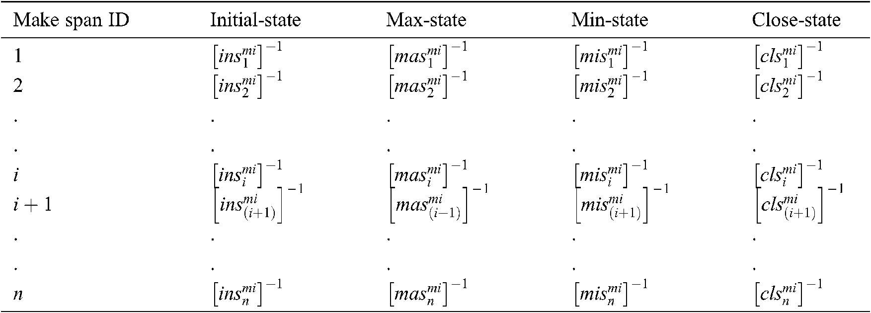
Further, for each metric {turnaround time interval, task arrival time interval, process completion time interval}, we shall find the moving averages of each status measure (initial-state, max-state, min-state, close-state).

For each column c of the two-dimensional matrix M(ins),M(mas),M(mis), or M(cls) representing status measures ins,mas,mis,andcls of each metric {turnaround time interval (tti) , task arrival time interval (tati) , process completion time interval (pcti) }, shall find moving averages of each column c

mai(c)=1mac∗(∀i=1(|c|−mac)⁡{∑j=imac{c[j]}}) // Moving average of the column c of the two-dimension matrix M of the metric tti,tati,orpcti

Further, each set of moving averages shall generate Bollinger bands to identify the potential volatility of load at the corresponding virtual machine.

4  Experimental Study

Regarding the experimental study execution, the preferential metric chosen for the model is energy consumption values. Thus, the metric for calculation covered in the system is for “Le” for a make-span.

The data in terms of units of energy consumed for the time frame T is considered for the experimental study as Instance-1 (depending on the cloud environment and load factors, the instance-1 could be presumed for different timelines. For experimental purpose, it is seen as an instance, and undefined timeframe).

The following stands the 50 instance values generated over the random value of energy consumption for a specific cloud server. The first 20 closing values are used for generating the random values for two virtual machines as a comparison. Considering the scope of experimental analysis, the model refers to the conditions wherein the Le values are chosen for two different Virtual machines for a simple figurative representation of the impact.

Figure 3: Ideally, the V1 is touching the bandwidth of higher volatility, and the V2 machine is closing towards the lower energy capacities

In the instances of Fig. 3 representation, ideally, the V1 is touching the bandwidth of higher volatility, and the V2 machine is closing towards the lower energy capacities. Thus, it is ideal for the resource scheduling algorithm to choose the V1 machine for allocation, despite reaching out to the higher capacities of energy consumption. The rationale stands that the V2-machine is much lower than the average conditions, and it could run out of energy capacity during the task of handling the resource, and it might have a disruption in the services. The discussed scenario of the resource scheduling model can be adapted as a top layer for the models of make-span algorithms in silos or combination with the other metrics.

The metrics used to scale the performance of the BBLB are “make-span rate”, “average of the turnaround time interval of a constant set of virtual machines having variable load”, and “average turnaround time interval of a variable set of virtual machines having constant load”. The metric values obtained from BBLB and the contemporary model STLB have been compared and analyzed. The descriptions related to the metric values obtained from BBLB, STLB, and their competency have presented in the following.

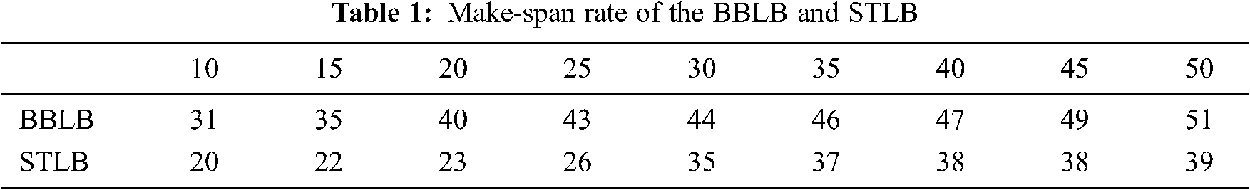
Figure 4: The make-span rate of the BBLB and STLB

The virtual machine’s availability or its fewer load scope denotes by the metric “make-span rate”. The higher values reflect the competency of the metric make-span rate. The more make-span rate represents the more availability of the corresponding virtual machine. The graph representation Fig. 4 of the Tab. 1 exibiting that the proposed BBLB has an average make-span rate of 43 ± 6, which is significantly higher than the average make-span rate of 30.5 ± 7.5 of the contemporary model STLB.

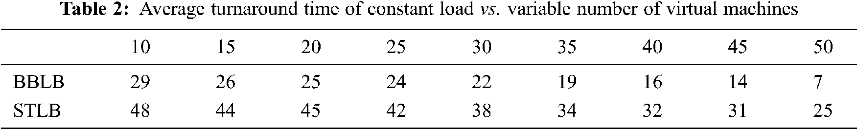
Figure 5: The average turnaround time intervals of BBLB and STLB versus the variable number of virtual machines

The average turnaround time intervals observed for the models BBLB and STLB against the variable count of virtual machines with constant load had been tabulated in Tab. 2, visualized in Fig. 5. The minimal values of the average turnaround time are optimal and competent to indicate the balanced load. The average turnaround time interval observed for BBLB is 20 ± 6.5, which considerably lower than the average turnaround time interval 38.0 ± 7.0 observed for contemporary model STLB.

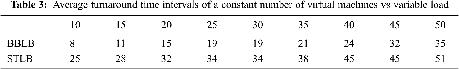
Figure 6: Turnaround time statistics of the models BBLB. And STLB against variable load

The average turnaround time intervals observed for the models BBLB and STLB against the constant count of virtual machines with variable load size had been tabulated in Tab. 3, visualized in Fig. 6. The minimal values of the average turnaround time are optimal and competent to indicate the balanced load. The average turnaround time interval observed for BBLB is 20.44 ± 8.4, which considerably lower than the average turnaround time interval of 36.88 ± 8.11 that was observed for contemporary model STLB.

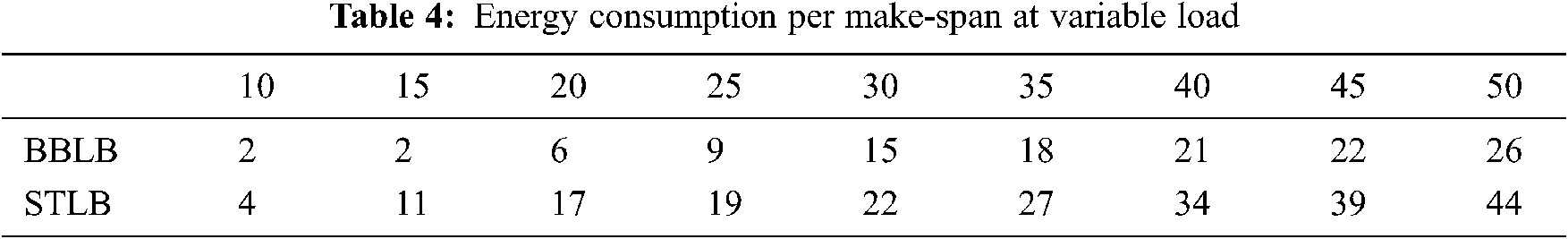
Figure 7: The metric average energy-consumption against variable load

Energy consumption is the other critical objective to achieve optimal load balancing decisions. Tab. 4 tabulated the average energy consumption per make-span against the variable load of both BBLB and STLB models, which have been figured as a bar graph in Fig. 7. The fewer values of the metric are more optimal and competent. The mean energy consumption of BBLB has been noted as 13.5 ± 8.5 jl , which is considerably lesser than the mean energy consumption of 24.11 ± 12.38 observed for the contemporary model STLB.

The model discussed in this study is compared to a model focused on load balancing in the cloud environment. The model considered for ideating the structure is STLB (Starvation Threshold-based Load Balancing), which balances the load based on the Starvation Threshold. In the model chosen for comparative analysis, the complexities of calculation for assessing load are intrinsic and are a tabulated composition that is complex for easy interpretation. Whereas the model proposed in this manuscript can reflect the figurative representation of the load factor for various VMs integral to a cloud computing environment.

5  Conclusion

Resource scheduling being a priority factor among the cloud computing requirements, there are numerous models and classified sets of resource scheduling algorithms being explored. Focusing on the volatility factor among the virtual machines to be engaged for resource allocation, this manuscript explores the contemporary approach of using the Bollinger Band model for statistical analysis of the load factor or the chosen metric for each of the virtual machine’s integral to the system. The critical advantage of the proposed system is its simplicity in the estimations, which do not require high computation times, and the decision-making process can be much simplified for allocation. The simulated experimental study of the model for a two-VM environment refers to the model’s potential to be implemented in large-scale cloud computing solutions. In addition, evolutionary technique, which shall use the visual indicators as the fitness function.

Acknowledgement: The authors extend their appreciation to the Deanship of Scientific Research at King Khalid University for funding this work through the General Research Project under grant number (R.G.P1/155/40).

Funding Statement: The authors extend their appreciation to the Deanship of Scientific Research at King Khalid University for funding this work under grant number (R.G.P-40-331), Received by Fuad A Al-Yarimi. https://www.kku.edu.sa.

Conflicts of Interest: The authors declare that they have no conflicts of interest to report regarding the present study.

References

 1.  S. Esmat, A. Badri and R. Ebrahimpour, “Decentralized multi-agent based energy management of microgrid using reinforcement learning,” Int. Journal of Electrical Power & Energy Systems, vol. 122, pp. 195–211, 2020. [Google Scholar]

 2.  K. Reihaneh and M. Ramezanpour, “An energy-efficient task-scheduling algorithm based on a multi-criteria decision-making method in cloud computing,” Int. Journal of Communication Systems, vol. 33, no. 9,pp. 79–84, 2020. [Google Scholar]

 3.  S. Singh and I. Chana, “QRSF: QoS-aware resource scheduling framework in cloud computing,” Journal of Supercomputing, vol. 71, no. 1, pp. 241–292, 2015. [Google Scholar]

 4.  L. Weiwei, X. Siyao, H. Ligang and L. Jin, “Multi-resource scheduling and power simulation for cloud computing,” Information Sciences, vol. 397–398, no. 4, pp. 168–186, 2017. [Google Scholar]

 5.  S. Singh and I. Chana, “A survey on resource scheduling in cloud computing: Issues and challenges,” Journal of Grid Computing, vol. 14, no. 2, pp. 217–264, 2016. [Google Scholar]

 6.  S. Dhahbi, M. Berrima and F. Al-Yarimi, “Load balancing in cloud computing using worst-fit bin-stretching,” Cluster Computing, vol. 22, pp. 1–15, 2020. [Google Scholar]

 7.  S. Varshney and S. Singh, “A survey on resource scheduling algorithms in cloud computing,” Int. Journal of Applied Engineering Research, vol. 13, no. 9, pp. 6839–6845, 2018. [Google Scholar]

 8.  S. Madni, M. Abd Latiff, Y. Coulibaly and S. Abdulhamid, “Resource scheduling for infrastructure as a service (IaaS) in cloud computing: Challenges and opportunities,” Journal of Network and Computer Applications, vol. 68, no. 1, pp. 173–200, 2016. [Google Scholar]

 9.  M. Bhatu Gawali and S. K. Shinde, “Task scheduling and resource allocation in cloud computing using a heuristic approach,” Journal of Cloud Computing, vol. 7, no. 4, pp. 1–16, 2018. [Google Scholar]

10. Y. Liu, L. Wang, X. Vincent Wang, X. Xu and L. Zhang, “Scheduling in cloud manufacturing: State-of-the-art and research challenges,” Int. Journal of Production Research, vol. 57, no. 15–16, pp. 4854–4879, 2019. [Google Scholar]

11. I. Strumberger, N. Bacanin, M. Tuba and E. Yube, “Resource scheduling in cloud computing based on a hybridized whale optimization algorithm,” Applied Sciences, vol. 9, no. 22, pp. 4893, 2019. [Google Scholar]

12. P. Devarasetty and C. Satyananda Reddy, “Research of task management and resource allocation in cloud computing,” Int. Journal of Innovative Technology and Exploring Engineering, (IJITEE), vol. 8, no. 6S4, pp. 938–941, 2019. [Google Scholar]

13. J. Chen, J. Xu and B. Hui, “Cloud computing resource scheduling based on improved semantic search engine,” in Proc. of the 2nd Int. Conf. on Intelligent Information Processing, Bangkok Thailand, pp. 1–5, 2017. [Google Scholar]

14. A. Hayes, “Bollinger band definition,” Technical Analysis Basic Education, 2019. [Online]. Available: https://www.investopedia.com/articles/technical/102201.asp. [Google Scholar]

15. A. Semmoud, M. Hakem, B. Benmammar and J. Charr, “Load balancing in cloud computing environments based on adaptive starvation threshold,” Concurrency and Computation: Practice and Experience, vol. 32, no. 11, pp. e5652, 2020. [Google Scholar]

This work is licensed under a Creative Commons Attribution 4.0 International License, which permits unrestricted use, distribution, and reproduction in any medium, provided the original work is properly cited.