Computer Systems Science & Engineering DOI:10.32604/csse.2022.020307
Article

Modified Mackenzie Equation and CVOA Algorithm Reduces Delay in UASN

R. Amirthavalli1,*, S. Thanga Ramya2 and N. R. Shanker3

1Department of Computer Science and Engineering, Velammal Engineering College, Chennai, 66, India
2Department of Information Technology, R. M. D Engineering College, Tiruvallur, 1206, India
3Department of Computer Science and Engineering, Aalim Muhammed Salegh College of Engineering, Chennai, 55, India
*Corresponding Author: R. Amirthavalli. Email: amirthavallisenthil@gmail.com
Received: 19 May 2021; Accepted: 06 July 2021

Abstract: In Underwater Acoustic Sensor Network (UASN), routing and propagation delay is affected in each node by various water column environmental factors such as temperature, salinity, depth, gases, divergent and rotational wind. High sound velocity increases the transmission rate of the packets and the high dissolved gases in the water increases the sound velocity. High dissolved gases and sound velocity environment in the water column provides high transmission rates among UASN nodes. In this paper, the Modified Mackenzie Sound equation calculates the sound velocity in each node for energy-efficient routing. Golden Ratio Optimization Method (GROM) and Gaussian Process Regression (GPR) predicts propagation delay of each node in UASN using temperature, salinity, depth, dissolved gases dataset. Dissolved gases, rotational and divergent winds, and stress plays a major problem in UASN, which increases propagation delay and energy consumption. Predicted values from GPR and GROM leads to node selection and Corona Virus Optimization Algorithm (CVOA) routing is performed on the selected nodes. The proposed GPR-CVOA and GROM-CVOA algorithm solves the problem of propagation delay and consumes less energy in nodes, based on appropriate tolerant delays in transmitting packets among nodes during high rotational and divergent winds. From simulation results, CVOA Algorithm performs better than traditional DF and LION algorithms.

Keywords: Gaussian process regression (GPR); golden ratio optimization method (GROM); corona virus optimization algorithm (CVOA); water column variation; dissolved gases; acoustic speed; divergent wind; rotational wind

1  Introduction

UASN plays a vital role in monitoring and surveillance of ocean areas in various depths. The monitoring and surveillance applications such as pollution monitoring, underwater exploration, seismic exploration, underwater navigation and tracking, hydrography, oceanography, Unmanned Underwater Vehicle (UUV), anti-submarine warfare needs efficient routing algorithms in different ocean environments and water column variations. The ocean environments are depth, salinity, temperature, and pressure. The water column variations are geometric and Doppler effects, rotational and divergent wind stress, dissolved gases, and sedimentation drift. Data transmission in water column variation is a challenging task in UASN, due to frequent variations in the water column such as dissolved gas and rotational and divergent wind stress. Efficient methodologies are needed for prediction and measurement of the ocean environment and water column parameters. However, algorithms such as VODA [1], RVPR [2], glider-assist routing [3], DVOR [4], DQELR [5], RCAR [6], DSR-SDN [7], EBOR [8] are having efficient routing in different ocean environmental conditions, whereas for water column variations such as geometric spread, sedimentation drift, and Doppler effect has only few UASN algorithms such as COCAN, LOCAN [9] are proposed. In UASN, acoustic signals perform better than extreme Low frequencies (ELF) due to less attenuation in underwater.

Data transmission between underwater sensor nodes depends on the water column, sound speed profile, and dissolved gases in the sea. Data transmission and routing in UASN is influenced by ocean parameters such as temperature, salinity, pressure, and depth of the sea. The pressure in the ocean increases as depth increases, dissolved gases vary according to the depth of the ocean. The dissolved gases are high for low salinity water, higher the pressure leads to higher dissolved gases in seawater. With the decrease in temperature, dissolved gases are higher. The dissolved CO2 concentration is proportional to the acoustic speed. Apart from CO2, the other gases such as H2S, CH4, and NH3 in water affects the data transmission in UASN. Moreover, the data transmission varies for different ocean depths due to different concentration of gases. The speed of sound is very fast for high temperature and low for thermocline regions where the temperature drops. Similarly, the speed of sound is proportional to pressure. The sound travels at a high speed in distilled water compared to ocean water. The high speed of sound in the ocean leads to high data transmission. The Speed of sound depends on ocean temperature. For example, the speed of sound increases by 4 m/s with a 1-degree increase in temperature, such an increase in temperature improves channel bandwidth during data transmission.

1.1 Problem Statement

In UASN, data transmission is affected due to water column variations, pressure, depth, salinity, temperature, sound profile, and dissolved gases. Many researchers developed various routing algorithms for data transmission in UASN. The existing routing algorithms measures each parameter with a specific sensor as optode, NDIR [10] is used for sensing dissolved gases. However, the energy consumption of sensors in the node is more and need an alternative approach for measurement. For example, the optode sensor consumes 1.8 W of power, and the response time for providing the result is about 3 min. Similarly, delay in data transmission arises in underwater due to divergent and rotational wind environments. Nodes in UASN needs efficient algorithm for prediction of ocean parameters such as divergent, rotational wind environment. Furthermore, the number of sensors in nodes needs to be replaced with an empirical method of calculation of dissolved gases in underwater and prevent more power consumption in each node. The delay in the response time of each sensor leads to more delay in UASN, which needs to be addressed along with divergent and rotational wind environment.

1.2 Contributions

Nodes in UASN needs a smaller number of sensors to reduce battery consumption. There are various sensors for measuring the depth, temperature, pressure, salinity, wind direction, dissolved gas, wind speed, sedimentation drift, Doppler Effect, and geometric spread. These sensors in a single node will consume more energy, more response time and delay in packet delivery. To reduce the number of sensors in node and improve the energy efficiency of the node through an empirical approach, the speed of sound in underwater is estimated through the Mackenzie equation. Mackenzie equation replaces sensors such as wind, wind direction, sedimentation drift, Doppler Effect, and geometric spread through the sound profile calculation obtained from the Mackenzie equation. In this paper, a Modified Mackenzie equation (MME) is proposed for the estimation of dissolved gases. Modified Mackenzie equation replaces sensors in node and estimates parameters of the ocean environment. In UASN, routing based on water column variations especially for divergent and rotational wind environments are yet to be designed. With this as an inspiration, this paper proposes a novel routing protocol that takes into account the ocean's parameters like dissolved gases, depth, salinity, temperature, rotational, and divergent wind stress.

1.    MME calculates the sound velocity of the node region, which includes dissolved gases. The node in the region needs an average sound velocity of 1527 m/s is selected for routing. MME helps to calculate the divergent and rotational wind through sound profile with Weather Observations through Ambient Noise (WOTAN). So, a sensor such as optode, NDIR is not required in each node.

2.    GROM and GPR predicts propagation delay of the nodes during the rotational and divergent wind stress in ocean based on Dataset.

3.    CVOA algorithm is applied for routing in UASN to avoid propagation delay due to dissolved gases, sedimentation drift, and water column variations.

2  Related Work

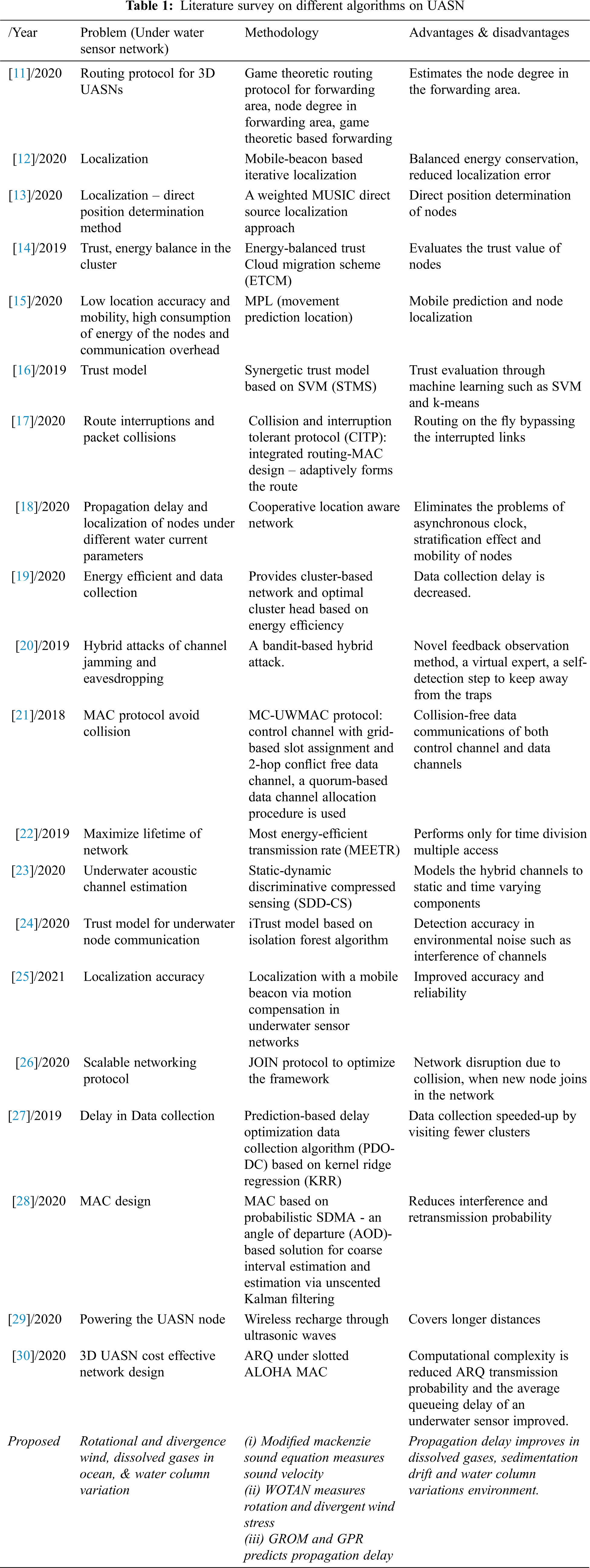
The Tab. 1 shows different algorithms in UASN and its advantages and disadvantages

3  Methodology

In recent years, routing algorithms are proposed for UASN based on location-based and depth-based. These routing algorithms never consider physical properties such as dissolved gases and effects of sound velocity during underwater data transmission. Sound velocity in dissolved gases play a vital role in underwater communication for efficient data transmission. In this paper, Modified Mackenzie Sound Equation based sound velocity measurement, Gaussian process regression based CVOA (GPR-CVOA), and Golden Ratio Optimization Method Based CVOA (GROM-CVOA) algorithms are proposed for routing in dissolved gases with divergent wind environment for reducing propagation delay. The proposed GPR-CVOA and GROM-CVOA considers underwater parameters such as temperature, depth, salinity, pressure, along with major underwater parameters such as sound velocity, rotational, divergent wind, and dissolved gases for routing and avoids propagation delay. For calculating sound velocity, the modified Mackenzie equation uses the above underwater parameters. The traditional Mackenzie equation considers only depth, salinity, and temperature, whereas the proposed modified Mackenzie equation in this paper, includes parameters such as dissolved CO2 and computes acoustic velocity. Acoustic velocity is predicted for each node in the network for knowing environment behaviors and estimates propagation delay through GPR or GROM due to dissolved gases and acoustic velocity underwater. The nodes in a high acoustic velocity environment are selected for data transmission. In each node, the modified Mackenzie equation calculates sound velocity for every 30 min and updates each node's database in UASN. The node's database consists of the following sensor-measured parameters such as temperature, dissolved gases, depth, and salinity and estimated parameters such as sound velocity, rotational wind stress, and divergent wind stress. The Sound velocity is measured through a modified Mackenzie equation. Through Sound velocity, rotational, divergent wind stress measured with Weather Observations through Ambient Noise (WOTAN) estimation equation as discussed in the following section [31]. Each node database is collected and applied in GPR or GROM for identification of propagation delay of each node based on the water column environment. The propagation delay is estimated for each node and stored in each node's database once in every 30 min. Nodes with less propagation delay are selected for routing by the CVOA algorithm. However, propagation delay changes among the selected nodes, and such changes are handled through delay-tolerant method of transmitting data in UASN. Fig. 1 shows Modified Mackenzie Sound Equation, Gaussian process, and Golden Ratio Optimizations Based CVOA Algorithm Routing implementation in UASN.

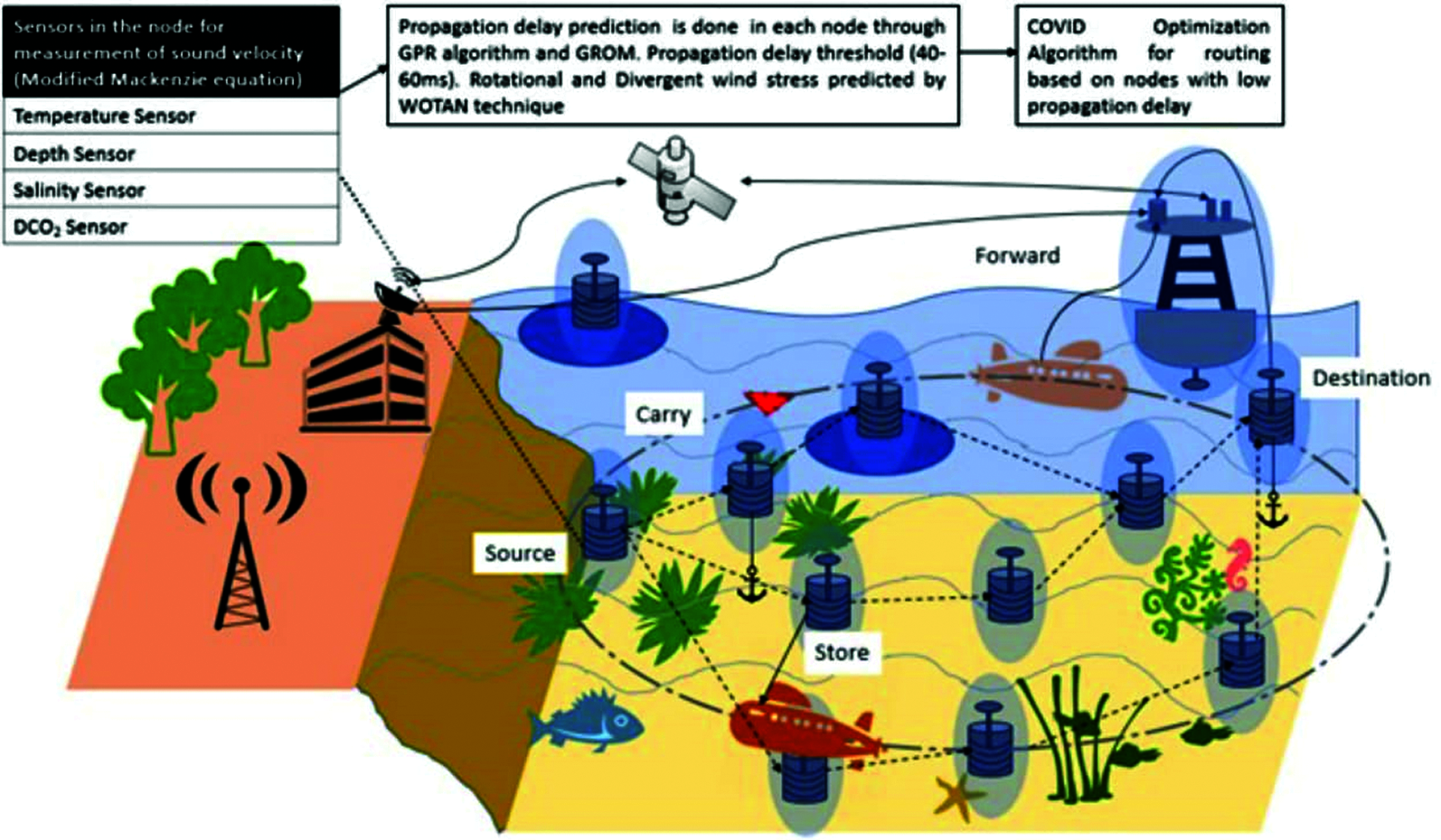
Figure 1: Modified mackenzie sound equation, gaussian process and golden ratio optimizations based CVOA algorithm routing in UASN

3.1 Modified Mackenzie Equation (MME)

Mackenzie Equation is as in Eq. (1) and measures c=acoustic velocity based on the T, S, and D.

C(D,}S,T)=1448.96+4.591T−5.304×10−2T2+2.374×10−4T3+1.340(S−35)+1.630×10−2D+1.675×10−7D2−1.025×10−2T(S−35)−7.139×10−13TD3 (1)

where T = temperature in degrees Celsius, S = salinity in parts per thousand, D = depth in meters, above equation is modified as in Eq. (2)

C(D, S, T, (DCO2))=1448.96+4.591T−5.304×10−2T2+2.374×10−4T3+1.340(S−35)                                               +1.630×10−2D+1.675×10−7D2−1.025×10−2T(S−35)                                              −7.139×10−13TD3+f(DCO2) (2)

where f(DCO2) = function of dissolved CO2. f(DCO2) represents the linear relationship between the dissolved CO2 and acoustic speed in seawater, such that the acoustic speed increases by 1.0 m/sec for every 2.5 mmol of dissolved CO2.

3.2 Weather Observations Through Ambient Noise (WOTAN)

In each node, environmental parameters such as temperature, depth, salinity, dissolved gases, pressure, and sound velocity, is measured, and then rotational, and divergent wind is measured through WOTAN. WOTAN measures wind speed based on underwater ambient noise. Underwater ambient noise is produced due to the excitations on ocean/sea surface and changes in weather conditions. WOTAN measures rotational, divergent wind stress estimated through the linear relationship between sound velocity pressure and surface wind speed is exploited and measures wind speed, which is given as in Eq. (3):

sv=o+(m∗sws) (3)

where sv – sound velocity pressure measured by μPa, o is offset, measured by μPa, m is slope, measured by μPa m−1s and sws is surface wind speed, measured by ms−1.

The sound pressure level 3 kHz 1/3-octave band shows an active response to the speed of wind which varies from 2 to 21.5 m/s. 21.5 m/s is characterized as a strong wind level.

3.3 Gaussian Process Regression (GPR)

Every node has a dataset of all parameters such as temperature, depth, salinity, dissolved gases, pressure, sound velocity (MME), is measured rotational, and divergent wind (WOTAN) then process with GPR for propagation delay estimation. Fig. 2 depicts the relationship between depth and acoustic speed. Fig. 3 shows the relationship between temperature and acoustic speed. Fig. 4 shows the relationship between salinity and acoustic speed.

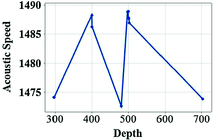
Figure 2: Acoustic speed (m/sec2) vs. depth (m)

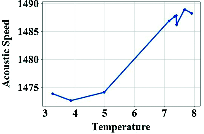
Figure 3: Acoustic speed (m/sec2) vs. temperature (C)

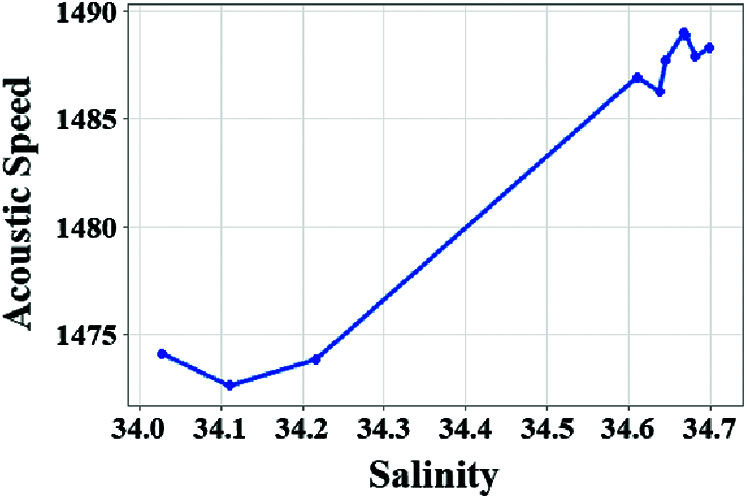
Figure 4: Acoustic speed (m/sec2) vs. salinity (PSU)

Gaussian Process Regression (GPR) is a nonparametric regression model and uses the Bayesian concept. GPR provides a better prediction for small datasets and provides the prediction's uncertainty estimation. GPR distribution infers from function. Gaussian processes are treated as a prior to build predictive posterior distribution given by Eq. (4).

f(x)  ∼GP(m(x),k(x,x′)) (4)

where m(x) is the mean function and k(x, x’) is a covariance function. The Squared exponential kernel or covariance function models smooth functions. The Squared exponential kernel provides infinitely many derivatives from prior functions, which is given by Eq. (5).

k(x,x′)=σ2exp(−(x−x′)22l2) (5)

where l smoothens the function and the output variance, σ2 checks the variation of function vertically.

The Eq. (6) shows relationship of acoustic velocity with depth, temperature and salinity.

C=1441.7913+0.0174×D+4.2254×T+0.1668×S (6)

where c is acoustic speed, D is depth, T is temperature, and S is salinity.

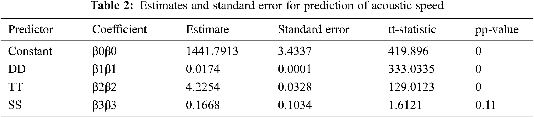
Tab. 2 shows the estimate and standard error for the regression model for acoustic speed and its predictors depth, temperature, and salinity.

Tab. 3 depicts the overall fit for the above discussed parameters

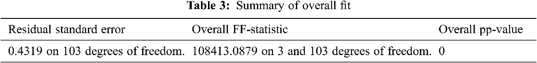
Fig. 5 shows histogram of residuals.

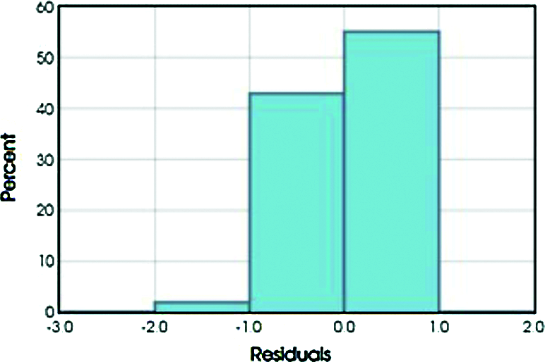
Figure 5: Histogram of residuals

Fig. 6 shows normal probability of residuals.

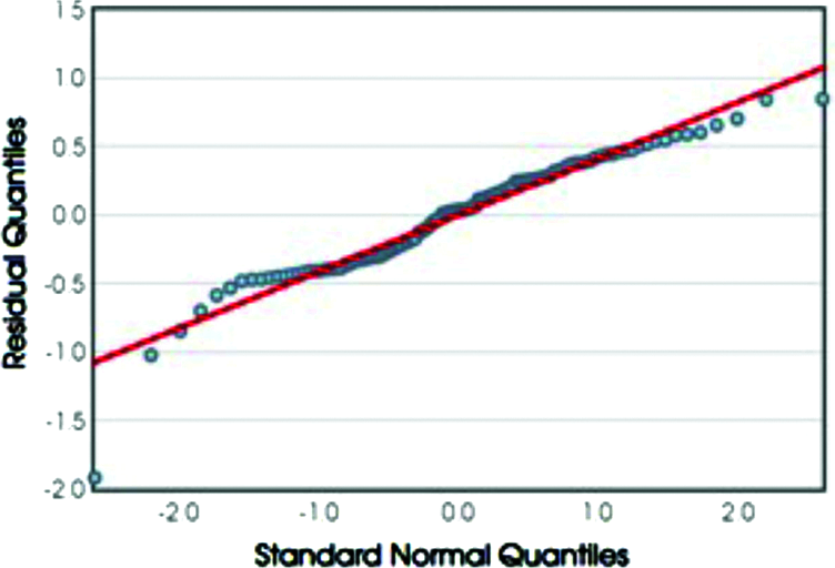
Figure 6: Normal probability of residuals

GPR predicts the nodes with low propagation delay.

3.4 Golden Ratio Optimization Method (GROM)

GROM is a parameter-less meta-heuristic optimization method, which is inspired by the golden ratio or golden mean found in the growth of plants and animals [32]. Fibonacci, a renowned mathematician, formulated this ratio by a series of numbers generated from the sum of the previous two numbers. Except for the first two numbers, all other numbers can be generated. The ratio of any two consecutive numbers is approximately the same i.e., 1.618, and represented as Ф. This kind of pattern is common in the arrangement of petals in flower, leaves, pinecones, shells, hurricanes. Any kth number x (a number in the Fibonacci series), such that k >= 3, in the Fibonacci series is generated by using this golden ratio, 1.618, which is given by Eq. (7):

xk=Φk−(1−Φ)k5 (7)

In GROM, the fitness mean of the population is computed and compared with the worst solution. To increase the speed of convergence, worst solution is replaced by the mean solution, if the fitness of the mean solution is better than the worst solution. A random vector from the population is selected for each vector population. The fitness of these two vectors is compared with the mean solution. The solutions are arranged as xbest, xmedium and xworst. The direction of movement of vectors and amount of movement is given by Eq. (8).

→xt=→xmedium−→xworst (8)

The fitness function is given by Eq. (9)

Ft=GF×ΦT−(1−Φ)T5 (9)

where GF = 1.618 and T = t/tmax, t and tmax are iterations to perform global search initially and then to search locally at the end.

The new vector is computed as in Eq. (10)

xnew=(1−Ft)×xbest+rand ×Ft×xt (10)

Based on boundary conditions, xnew replaces the original solution, if the computed new solution is better than the original. The second phase attempts to move for solutions closer to the best solution based on Eq. (11),

xnew=xold+rand×(1GF)×(xbest−xworst) (11)

where, 1/GF = 0.618

The boundary conditions are checked and the old vector replaces the newly computed values if the new vector is better than the old one.

3.5 Corona Virus Optimization Algorithm (CVOA)

In recent times, many metaheuristic algorithms inspired by nature is proposed and finds the optimal solution for different problems. COVID-19, Corona Virus Optimization algorithm (CVOA) [33] is one such metaheuristic algorithm, which simulates Coronavirus spread and infects healthy individuals. Patient zero (PZ) is the first infected individual, spreads the virus to other healthy individuals. The infected individual may either die or spread infection. Initially, the infection spreads exponentially and later decrease due to recovery or deaths in the population. The disease propagates from PZ. The initial population is generated with prime infected individual PZ. PZ infects other individuals in the population. Each infected individual die either based on probability P_DIE or spread infection. Based on probability P_SUPERSPREADER, spreaders are differentiated into Ordinary spreaders and Super-spreaders. The ordinary spreader spreads infection based on SPREADING_RATE, whereas super-spreader infects population-based on SUPERSPREADING_RATE. CVOA assumes some of the infected individuals travel for diversification. Each infected individual travel with probability P_TRAVEL. Based on this probability, the infected individual either travels with TRAVELER_RATE or if not travels in ORDINARY_RATE. An infected individual can be both a super-spreader or a traveler.

In each generation, three types of population namely deaths, recovered, the new infected population are observed and updated. The dead individuals are added to this population and cannot be reused. At the start of every iteration, all infected populations are added to the recovered population. The individual recovered can be reinfected with probability P_REINFECTION. When an individual is infected, he/she might be isolated to follow social distancing norms. Such isolated individuals may be added to the recovered population with probability P_ISOLATION. All infected population in each iteration is added to the new infected population. The stop criterion is a pre-set number of iterations. In initial iterations, infections will grow exponentially, along with it grows recovered population and dead population.

The below algorithm explains the use of the CVOA algorithm in UASN. In this paper, x is considered to be the PZ and Sedimentation drift causes rotational, divergent wind stress and considered to be the virus that affects the nodes in UASN. The sizeOf() returns the number of infected nodes and the noBattery() returns true if there is no charge remaining in the battery of the infected node and the node is considered dead. The infect () receives an infected node and returns the newly infected nodes into the system. The CVOA algorithm is as below in Tab. 4.

4  Results and Discussion

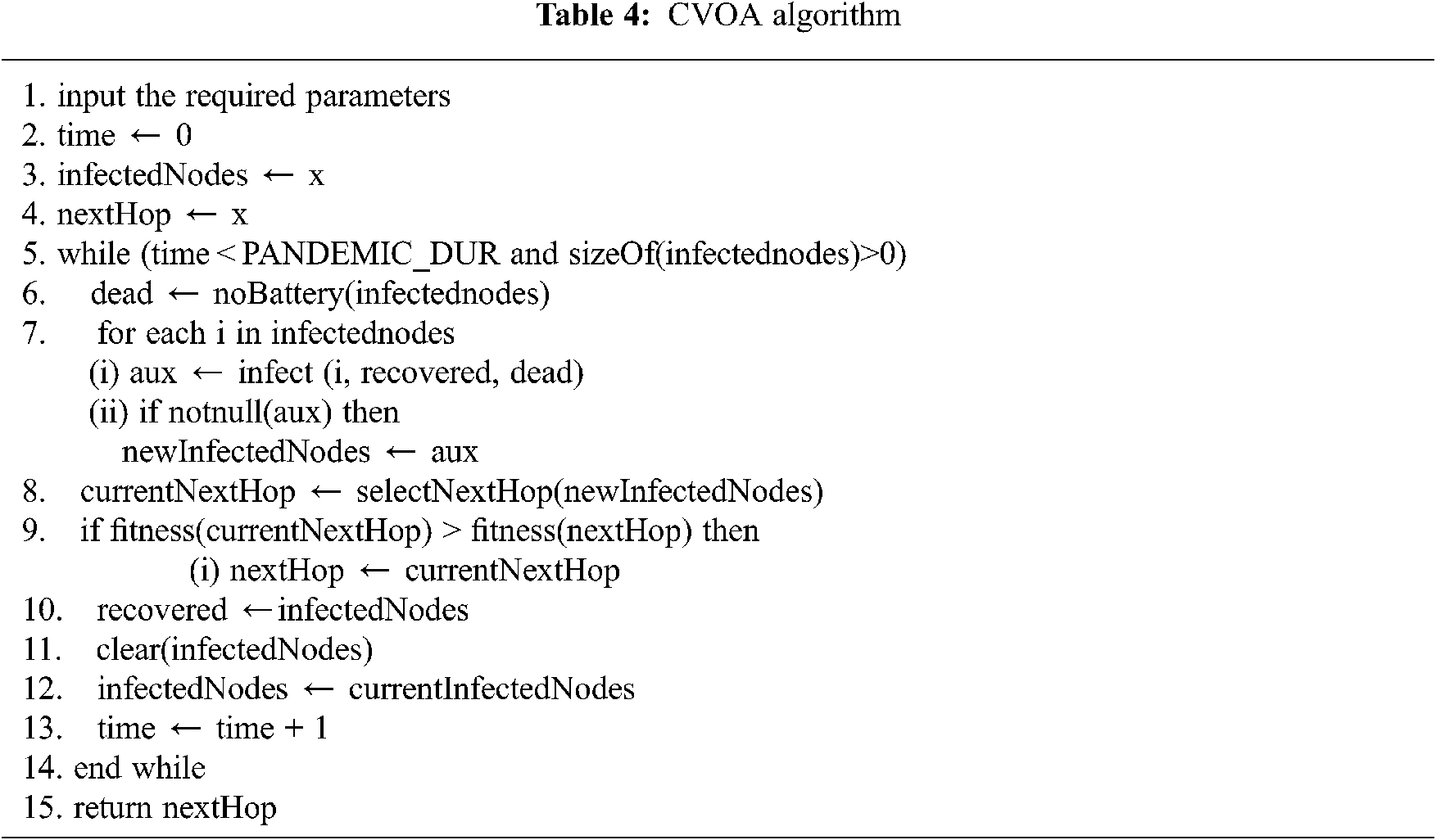
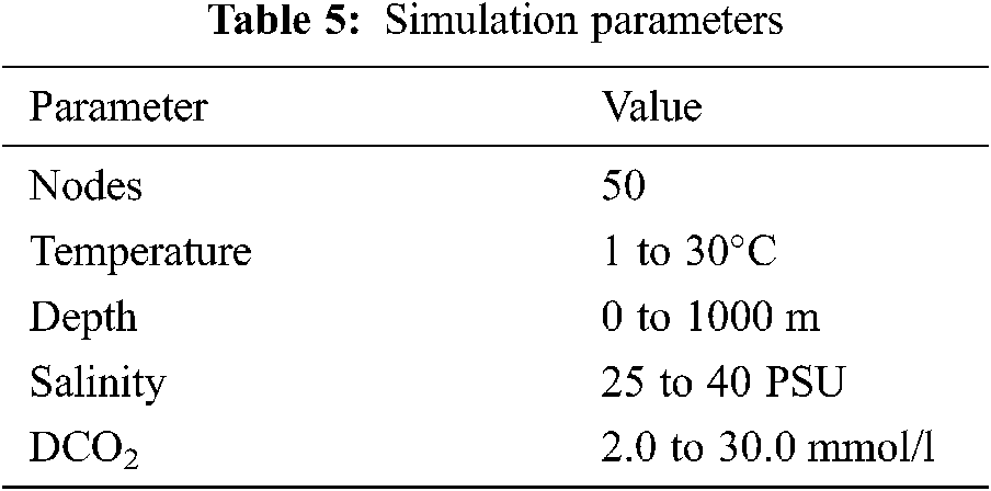
Fig. 7 shows the system model. NS2 AquaSim simulator is used to simulate the underwater acoustic environment. Tab. 5. shows the simulation parameters. For every 30 min, node parameters such as temperature, pressure, salinity, dissolved gases, rotational and divergent wind stress is estimated using Mackenzie equation and WOTAN estimation, such observed data are stored in node's database. The node with an acoustic velocity greater than 1527 m/sec is selected for the next step.

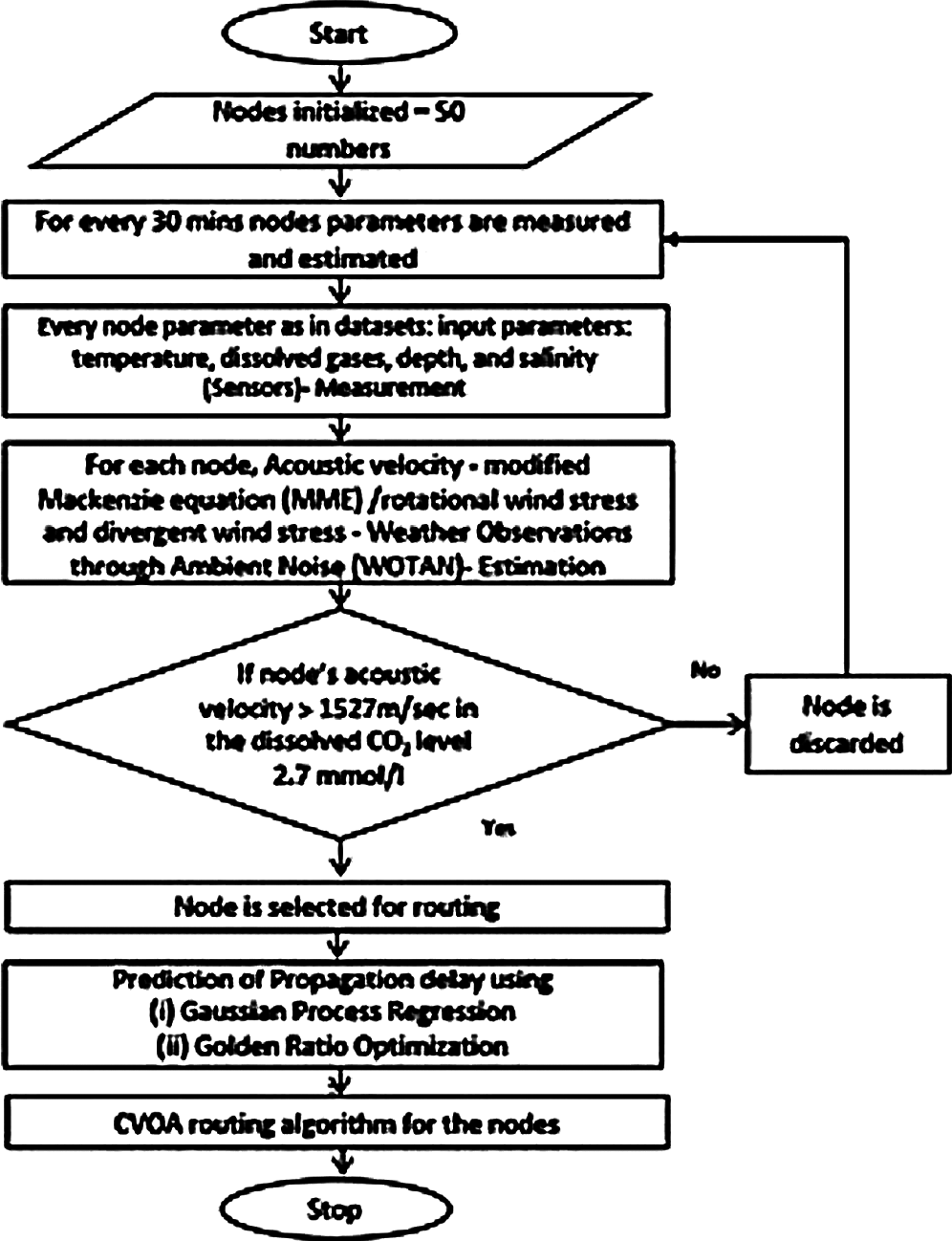
Figure 7: Routing using GPR, GROM and CVOA

In this paper, Gaussian Process calculates propagation delay in each node based on the database in respective node, and the nodes with less propagation delay are only considered for routing through the CVOA algorithm as shown in Fig. 8. However, the performance of the GPR in the prediction of propagation delay, in each node, is replaced with the GROM algorithm and then the CVOA algorithm is applied. The selection of nodes, through the GPR algorithm and GROM algorithm, plays a vital role for energy-aware routing in the network through appropriate node selections. The CVOA routing algorithm applied in two scenarios such as

1.    GPR and CVOA algorithm

2.    GROM and CVOA algorithm

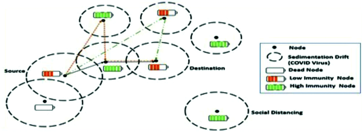
Figure 8: CVOA in UASN for routing

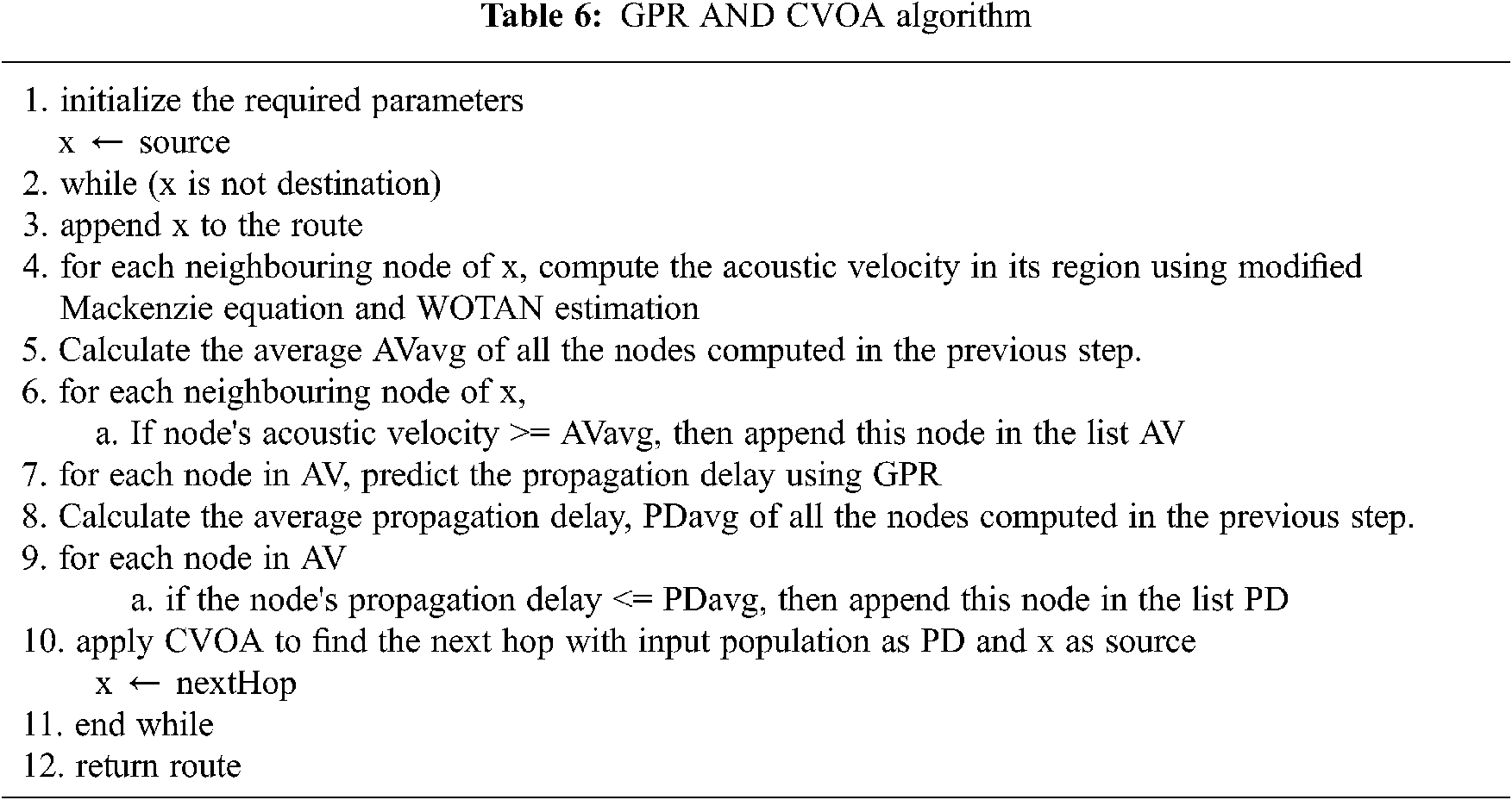
4.1 GPR and CVOA Based Routing

CVOA finds the best route after selecting the nodes with less propagation delay. The source is considered as PZ. Based on the acoustic velocity of each neighboring nodes’ region, the node is added to the UASN network.

Sedimentation drift causes rotational, divergent wind stress and considered to be the virus that affects nodes in the UASN. Each node is considered either as an ordinary spreader or a super-spreader considering its battery level. The node with a high battery is considered to have high immunity and considered to be an ordinary-spreader. The node with less battery level is a super-spreader as sedimentation drift drains the sensor battery. The node that has no battery left is considered as a dead node. If a node has a good acoustic velocity region and good battery level but away from the formed UASN, then that node is considered as a node maintaining social distancing and will not be part of the network. Fig. 8 shows the routing of CVOA.

The following Tab. 6 describes GPR and CVOA algorithm for routing selected nodes in UASN.

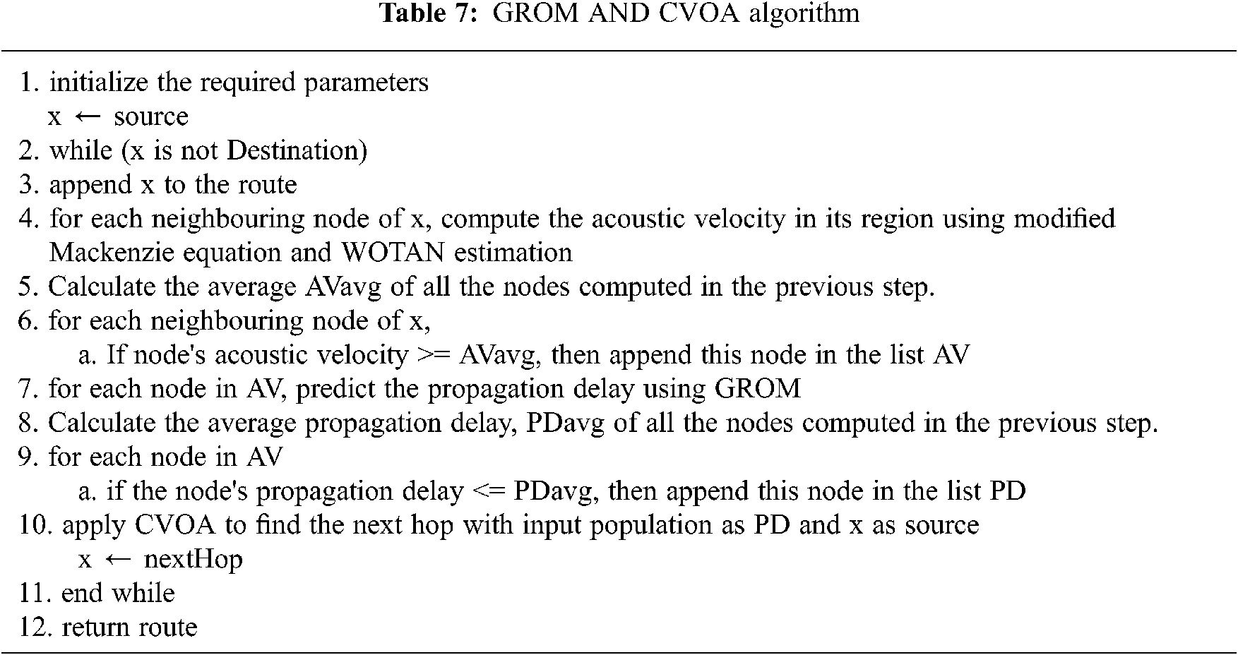
4.2 GROM and CVOA Based Routing

The following Tab. 7 describes GROM and CVOA algorithm for routing selected nodes in UASN.

The performance of GPR-CVOA and GROM-CVOA is compared with the Direct Forwarding (DF) algorithm and LION algorithm [10]. Fig. 9 illustrates the effects of the number of nodes on delay. GPR-CVOA is performing better when compared to DF, GROM-CVOA, and LION. Fig. 10 analyses energy consumption when the number of nodes varies. It is observed that energy consumption reduces as the number of nodes in the network increases. The energy consumption of GROM-CVOA is close to that of the LION protocol's energy consumption. Energy consumption is less in GPR-CVOA, GROM-CVOA than DF and LION. Fig. 11 expresses the relationship between acoustic speed and delay and they are inversely proportional to each other. GPR-CVOA outperforms other algorithms and has minimal delay than other protocols like GROM-CVOA, DF, and LION. Fig. 12 illustrates throughput vs. the number of nodes. The graph shows that GPR-CVOA has more throughput when compared to other protocols. Fig. 13 illustrates the effect of dissolved gases vs. acoustic speed. Fig. 14 shows the effects of the number of nodes on PDR is analyzed. Both GPR-CVOA and GROM-CVOA protocols has better PDR than LION and DF. Both GPR-CVOA and GROM-CVOA protocols has a good initial PDR than DF as water-column properties, dissolved gases, wind patterns are accounted for while calculating the route for packet transmission. Fig. 15 illustrates Normalized Routing Overhead (NRO) versus time. NRO is less in GPR-CVOA and GROM-CVOA than DF and LION. Fig. 16 shows that in presence of rotational wind, propagation delay increases with an increase in the number of nodes. The GPR-CVOA and GROM-CVOA protocols perform better than DF and LION. Fig. 17 illustrates the propagation delay versus the number of nodes in presence of divergent wind. GPR-CVOA performs well than the GROM-CVOA protocol but both are better than the other two protocols under study.

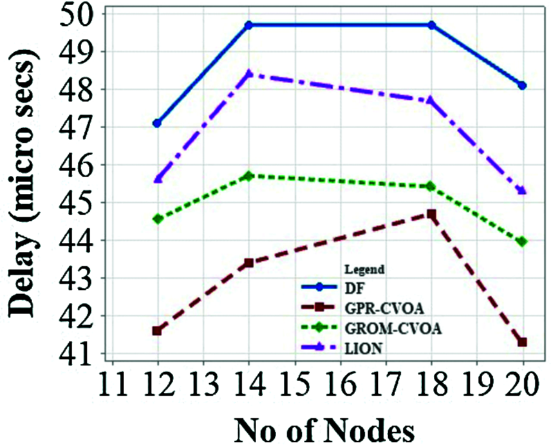
Figure 9: Delay vs. number of nodes

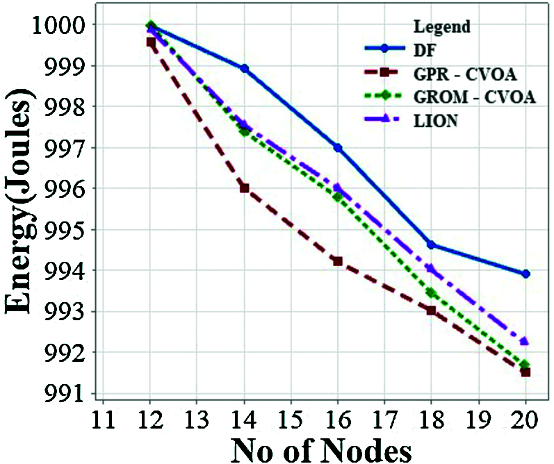
Figure 10: Energy vs. number of nodes

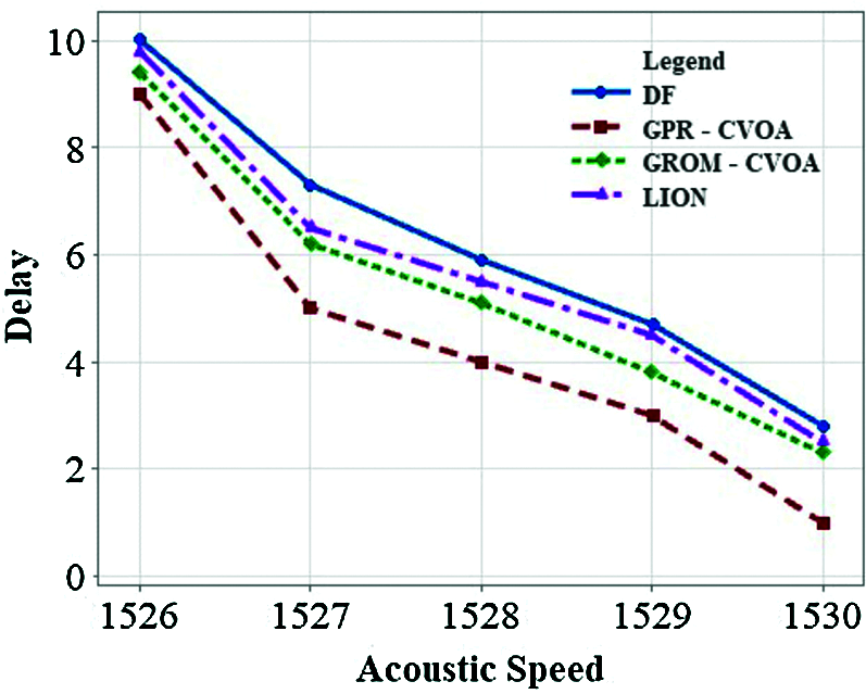
Figure 11: Acoustic speed vs. delay

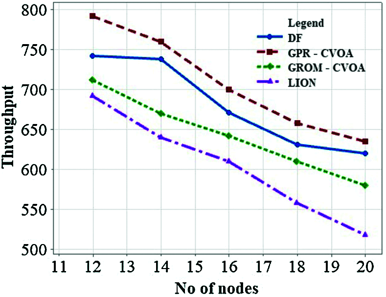
Figure 12: Throughput vs. number of nodes

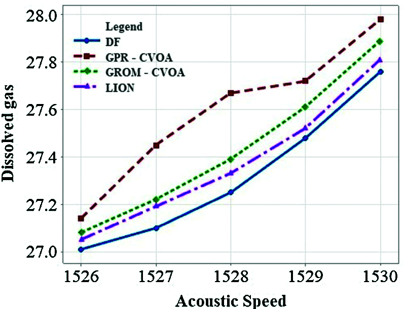
Figure 13: Dissolved gas vs. acoustic speed

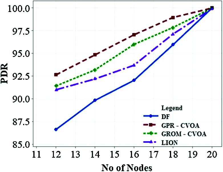
Figure 14: PDR vs. number of nodes

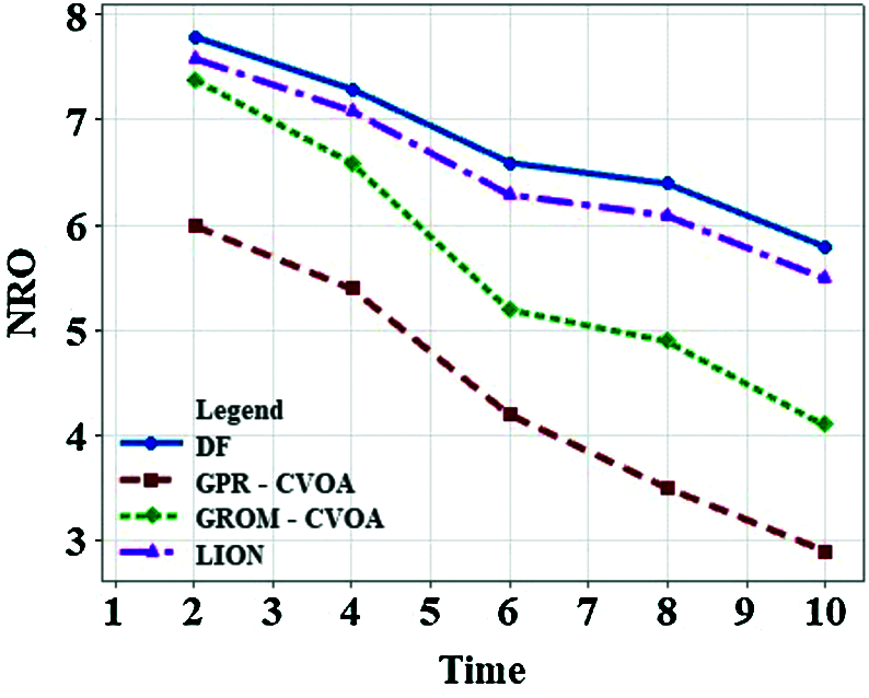
Figure 15: NRO vs. time (millisecs)

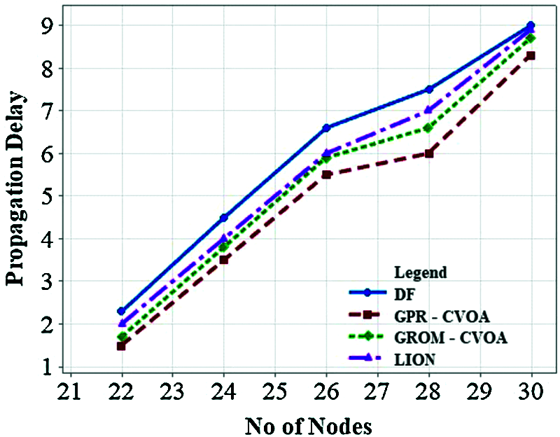
Figure 16: Propagation delay vs. number of nodes in the presence of rotational wind

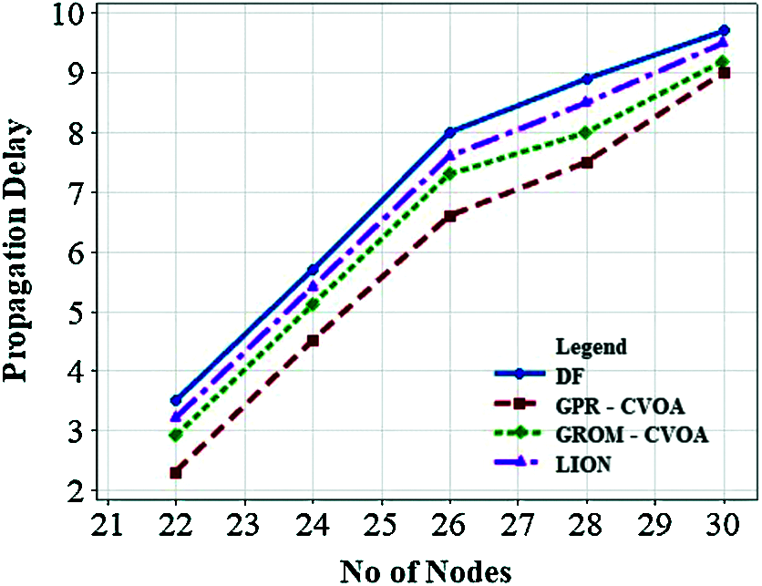
Figure 17: Propagation delay vs. number of nodes in the presence of divergent wind

Performance of GPR-CVOA and GROM-CVOA shows that under changing wind patterns and dissolved gases, protocols are robust and prove to be working better than DF and LION.

5  Conclusion

In UASN, routing and propagation delay is affected because of temperature, salinity, depth, dissolved gases, sound velocity, divergent and rotational wind. MME is proposed to calculate sound velocity in each node region, which includes dissolved gases. MME helps to calculate the divergent and rotational wind through sound profile with WOTAN. GROM and GPR predicts propagation delay of each node based on dissolved gases, rotational and divergent wind stress. Predicted values from GPR and GROM leads to node selection and among selected nodes CVOA routing is performed. The proposed GPR-CVOA and GROM-CVOA algorithm solves the problem of propagation delay and consumes less energy in nodes based on appropriate tolerant delays in transmitting packets among nodes during high rotational and divergent winds. The proposed algorithms perform better than existing water column variation algorithms. To reduce number of sensors in node and to improve the energy efficiency of the node, Mackenzie equation - empirical method is applied. Mackenzie equation replaces sensors such as wind, wind direction, sedimentation drift, Doppler Effect, and geometric spread through the sound profile calculation obtained from the Mackenzie equation. The prediction algorithm can be applied with deep learning algorithms for other water column variations, which consumes more power such as sand drift and turbulence.

Acknowledgement: We authors thank S. Tamilselvi for providing the valuable support towards ocean data collection and suggestions in water column variations.

Funding Statement: The authors received no specific funding for this study.

Conflicts of Interest: The authors declare that they have no conflicts of interest to report regarding the present study.

References

 1.  Y. Su, L. Guo, Z. Jin and X. Fu, “A voronoi-based optimized depth adjustment deployment scheme for underwater acoustic sensor networks,” IEEE Sensors Journal, vol. 20, no. 22, pp. 13849–13860, 2020. [Google Scholar]

 2.  Z. Jin, Q. Zhao and Y. Luo, “Routing void prediction and repairing in auv-assisted underwater acoustic sensor networks,” IEEE Access, vol. 8, pp. 54200–54212, 2020. [Google Scholar]

 3.  Y. Su, L. Zhang, Y. Li and X. Yao, “A glider-assist routing protocol for underwater acoustic networks with trajectory prediction methods,” IEEE Access, vol. 8, pp. 154560–154572, 2020. [Google Scholar]

 4.  Q. Guan, F. Ji, Y. Liu, H. Yu and W. Chen, “Distance-vector-based opportunistic routing for underwater acoustic sensor networks,” IEEE Internet of Things Journal, vol. 6, no. 2, pp. 3831–3839, 2019. [Google Scholar]

 5.  Y. Su, R. Fan, X. Fu and Z. Jin, “DQELR: An adaptive deep q-network-based energy- and latency-aware routing protocol design for underwater acoustic sensor networks,” IEEE Access, vol. 7, pp. 9091–9104, 2019. [Google Scholar]

 6.  Z. Jin, Q. Zhao and Y. Su, “RCAR: A reinforcement-learning-based routing protocol for congestion-avoided underwater acoustic sensor networks,” IEEE Sensors Journal, vol. 19, no. 22, pp. 10881–10891, 2019. [Google Scholar]

 7.  C. Lin, G. Han, M. Guizani, Y. Bi and J. Du, “A scheme for delay-sensitive spatiotemporal routing in SDN-enabled underwater acoustic sensor networks,” IEEE Transactions on Vehicular Technology, vol. 68, no. 9, pp. 9280–9292, 2019. [Google Scholar]

 8.  Z. Jin, Z. Ji and Y. Su, “An evidence theory based opportunistic routing protocol for underwater acoustic sensor networks,” IEEE Access, vol. 6, pp. 71038–71047, 2018. [Google Scholar]

 9.  A. Rajeswari, N. Duraipandian, N. R. Shanker and B. E. Samuel, “Improving packet delivery performance in water column variations through locan in underwater acoustic sensor network,” Journal of Sensors, vol. 2020, pp. 1–16, 2020. [Google Scholar]

10. J. S. Clarke, E. P. Achterberg, D. P. Connelly, U. Schuster, M. Mowlem, “Developments in marine pCO2 measurement technology; towards sustained in situ observations,” TrAC Trends in Analytical Chemistry, TrAC Trends in Analytical Chemistry, vol. 88, pp. 53–61, 2017. [Google Scholar]

11. Q. Wang, J. Li, Q. Qi, P. Zhou and D. O. Wu, “A game-theoretic routing protocol for 3-d underwater acoustic sensor networks,” IEEE Internet of Things Journal, vol. 7, no. 10, pp. 9846–9857, 2020. [Google Scholar]

12. Y. Su, L. Guo, Z. Jin and X. Fu, “A mobile-beacon-based iterative localization mechanism in large-scale underwater acoustic sensor networks,” IEEE Internet of Things Journal, vol. 8, no. 5, pp. 3653–3664, 2021. [Google Scholar]

13. L. Wang, Y. Yang and X. Liu, “A direct position determination approach for underwater acoustic sensor networks,” IEEE Transactions on Vehicular Technology, vol. 69, no. 11, pp. 13033–13044, 2020. [Google Scholar]

14. G. Han, J. Du, C. Lin, H. Wu and M. Guizani, “An energy-balanced trust cloud migration scheme for underwater acoustic sensor networks,” IEEE Transactions on Wireless Communications, vol. 19, no. 3, pp. 1636–1649, 2020. [Google Scholar]

15. W. Zhang, G. Han, X. Wang, M. Guizani, K. Fan et al., “A node location algorithm based on node movement prediction in underwater acoustic sensor networks,” IEEE Transactions on Vehicular Technology, vol. 69, no. 3, pp. 3166–3178, 2020. [Google Scholar]

16. G. Han, Y. He, J. Jiang, N. Wang, M. Guizani et al., “A synergetic trust model based on SVM in underwater acoustic sensor networks,” IEEE Transactions on Vehicular Technology, vol. 68, no. 11, pp. 11239–11247, 2019. [Google Scholar]

17. R. Zhao, N. Li, O. A. Dobre and X. Shen, “CITP: Collision and interruption tolerant protocol for underwater acoustic sensor networks,” IEEE Communications Letters, vol. 24, no. 6, pp. 1328–1332, 2020. [Google Scholar]

18. J. Yan, D. Guo, X. Luo and X. Guan, “AUV-Aided localization for underwater acoustic sensor networks with current field estimation,” IEEE Transactions on Vehicular Technology, vol. 69, no. 8, pp. 8855–8870, 2020. [Google Scholar]

19. X. Zhuo, M. Liu, Y. Wei, G. Yu, F. Qu et al., “AUV-Aided energy-efficient data collection in underwater acoustic sensor networks,” IEEE Internet of Things Journal, vol. 7, no. 10, pp. 10010–10022, 2020. [Google Scholar]

20. X. Li, Y. Zhou, L. Yan, H. Zhao, X. Yan et al., “Optimal node selection for hybrid attack in underwater acoustic sensor networks: A virtual expert-guided bandit algorithm,” IEEE Sensors Journal, vol. 20, no. 3, pp. 1679–1687, 2020. [Google Scholar]

21. F. Bouabdallah, C. zidi, R. Boutaba and A. Mehaoua, “Collision avoidance energy efficient multi-channel mac protocol for underwater acoustic sensor networks,” IEEE Transactions on Mobile Computing, vol. 18, no. 10, pp. 2298–2314, 2019. [Google Scholar]

22. Y. Zhou, H. Yang, Y. Hu and S. Kung, “Cross-layer network lifetime maximization in underwater wireless sensor networks,” IEEE Systems Journal, vol. 14, no. 1, pp. 220–231, 2020. [Google Scholar]

23. W. Jiang, F. Tong, S. Zheng and X. Cao, “Estimation of underwater acoustic channel with hybrid sparsity via static-dynamic discriminative compressed sensing,” IEEE Sensors Journal, vol. 20, no. 23, pp. 14548–14558, 2020. [Google Scholar]

24. J. Du, G. Han, C. Lin and M. Martinez-Garcia, “ITrust: An anomaly-resilient trust model based on isolation forest for underwater acoustic sensor networks,” IEEE Transactions on Mobile Computing, vol. 19, pp. 1–13, 2020. [Google Scholar]

25. Y. Kim, M. Erol-Kantarci, Y. Noh and K. Kim, “Range-free localization with a mobile beacon via motion compensation in underwater sensor networks,” IEEE Wireless Communications Letters, vol. 10, no. 1, pp. 6–10, 2021. [Google Scholar]

26. N. Morozs, P. D. Mitchell and R. Diamant, “Scalable adaptive networking for the internet of underwater things,” IEEE Internet of Things Journal, vol. 7, no. 10, pp. 10023–10037, 2020. [Google Scholar]

27. G. Han, S. Shen, H. Wang, J. Jiang and M. Guizani, “Prediction-based delay optimization data collection algorithm for underwater acoustic sensor networks,” IEEE Transactions on Vehicular Technology, vol. 68, no. 7, pp. 6926–6936, 2019. [Google Scholar]

28. M. Rahmati and D. Pompili, “Probabilistic spatially-divided multiple access in underwater acoustic sparse networks,” IEEE Transactions on Mobile Computing, vol. 19, no. 2, pp. 405–418, 2020. [Google Scholar]

29. R. Guida, E. Demirors, N. Dave and T. Melodia, “Underwater ultrasonic wireless power transfer: A battery-less platform for the internet of underwater things,” IEEE Transactions on Mobile Computing, vol. 19, pp. 30–42, 2020. [Google Scholar]

30. Y. Song, “Underwater acoustic sensor networks with cost fficiency for internet of underwater things,” IEEE Transactions on Industrial Electronics, vol. 68, no. 2, pp. 1707–1716, 2021. [Google Scholar]

31. P. Cauchy, K. J. Heywood, N. D. Merchant, B. Y. Queste, P. Testor, “Wind speed measured from underwater gliders using passive acoustics,” Journal of Atmospheric and Oceanic Technology, vol. 35, no. 12, pp. 2305–2321, 2018. [Google Scholar]

32. A. F. Nematollahi, A. Rahiminejad and B. Vahidi, “A novel meta-heuristic optimization method based on golden ratio in nature,” Soft Computing, vol. 24, no. 2, pp. 1117–1151, 2020. [Google Scholar]

33. F. Martínez-Álvarez, G. Asencio-Cortés, J. F. Torres, D. Gutiérrez-Avilés, L. Melgar-García et al., “Coronavirus optimization algorithm: A bioinspired metaheuristic based on the COVID-19 propagation model,” Big Data, vol. 8, no. 4, pp. 308–322, 2020. [Google Scholar]

This work is licensed under a Creative Commons Attribution 4.0 International License, which permits unrestricted use, distribution, and reproduction in any medium, provided the original work is properly cited.