DOI:10.32604/csse.2022.020020
| Computer Systems Science & Engineering DOI:10.32604/csse.2022.020020 | |
| Article |
A Smart Deep Convolutional Neural Network for Real-Time Surface Inspection
Department of Mechanical Engineering, Federal University of Technology, Parana, Curitiba, 81280-340, PR, Brazil
*Corresponding Author: Marco A. Luersen. Email: luersen@utfpr.edu.br
Received: 06 May 2021; Accepted: 15 July 2021
Abstract: A proper detection and classification of defects in steel sheets in real time have become a requirement for manufacturing these products, largely used in many industrial sectors. However, computers used in the production line of small to medium size companies, in general, lack performance to attend real-time inspection with high processing demands. In this paper, a smart deep convolutional neural network for using in real-time surface inspection of steel rolling sheets is proposed. The architecture is based on the state-of-the-art SqueezeNet approach, which was originally developed for usage with autonomous vehicles. The main features of the proposed model are: small size and low computational burden. The model is 10 to 20 times smaller when compared to other networks designed for the same task, and more than 700 times smaller than general networks. Also, the number of floating-point operations for a prediction is about 50 times lower than the ones used for similar tasks. Despite its small size, the proposed model achieved near-perfect accuracy on a public dataset of 1800 images of six types of steel rolling defects.
Keywords: Deep learning; surface defects classification; steel rolling
Steel sheets are one of the main products of iron and steel industry sector. They are produced by thousands a day, and some defects, such as surface crazing, inclusions, patches, pitting, rolled-in scale and scratches are almost unavoidable. Since these defects affect the sheet abrasion and corrosion resistance, fatigue strength and appearance, their proper detection and classification in real time have become a requirement for any production line. To fulfill these needs, computer vision and machine learning (ML) are slowly becoming the industry standard techniques for surface defect classification. However, computers used in the production line of small to medium size companies, in general, lack performance to attend real-time inspection with high processing demands. In these contexts, the use of models with small size and low computational burden, but still accurate, is an actual need.
Spanning from the early 1990’s until this date, many papers have addressed the challenges of automating visual quality control [1–6]. From the literature, it is clear that the paradigm of vision-based ML is slowly shifting from handcrafted codes such as feature extraction + classifier (support vector machines, or fully connected neural network) to more general approaches such as deep convolutional neural networks (DCNN).
A comprehensive study on support vector machines (SVM) for image classification can be found in the work of Burges [7]. This traditional way of image recognition relies deeply on feature engineering which in turn requires domain-specific expertise. The main arguments against this approach are: (1) need for feature engineering; (2) design of features is done separately from the classifier, complicating the process; (3) features may vary significantly from one application to another; (4) poor accuracy when compared to modern DCNN.
The two key ideas of deep learning for computer vision are the convolutional neural network and the backpropagation algorithm. Even though these theories were well developed by late 1980’s, only recently (around 2012) the technology was able to take off. The five main enabling technologies/causes are: (i) advances in graphical processing unit (GPU) computing, driven by the gaming industry; (ii) very large public datasets, mainly driven by the growth of the internet; (iii) better activation functions, weight initialization schemes and optimization algorithms; (iv) a wave of investment, both from public and private sources; and (v) democratization of knowledge.
With a basic knowledge of Python, R or any similarly high-level computer language, one can do almost anything with deep learning. This was driven mainly due to the development of symbolic tensor-manipulation frameworks such as Theano or TensorFlow. All this together brought a hype around deep learning in the past few years. A comprehensive review of the history of deep learning has been done by Schmidhuber [8]; for a gentle introduction to the technical details one can read the work of LeCun et al. [9]; and for a hands-on approach the books of Chollet [10] and Chollet et al. [11], which give the reader a fast paced introduction to deep learning with plenty of applications.
Several papers address the identification of surface defects using machine learning, some of them are briefly discussed in this section.
One of the first works that used DCNN for solving surface defects detection task is presented by Macsci et al. [12]. However, at that time (2012), this research field was relatively young and techniques limited. In that work it was proposed a simple architecture consisting in alternating convolutional and max-pooling layers followed by a two fully connected layers. This type of architecture was the standard one at early days of DCNN. Also, they used tanh activation functions in all layers but the last one, that used a softmax. Today, almost all deep networks use rectified linear units (ReLu) as activation function to avoid the vanishing gradient problem [13]. ReLu also provides low computational cost, which is one of the goals of the present work. Masci et al. [12] used stochastic gradient descent as the optimization scheme with annealed learning rate, however, none of the optimization parameters were disclosure. No regularization layer was used by the model, so that architecture is probably susceptible to overfitting. Indeed, the authors reported that reducing the model capacity, by freezing the weights of the first convolutional layer at random values, the generalization power of their network improved when not using data augmentation. To avoid overfitting issues, the authors used random translation of 15% as data augmentation. Their best-reported result was 93.03% of accuracy on a dataset that is not publicly available. That simple architecture is used as a performance baseline to our tests.
A similar, but more recent work, is presented by Zhou et al. [14]. They also use a standard DCNN to classify defects on steel sheets, but a model with much more capacity is used (more filters on the convolutional layer). The architecture is shown in Fig. 2. Since it is a recent work, the authors use dropout as regularization (standard technique nowadays). To reduce the computational burden by reducing network size, the authors re-scaled the input images from 200 × 200 to 40 × 40 using average pooling (window and stride of 5 × 5). For 200 training samples (similar size of what is performed on the present work) the authors reported an accuracy of 96.43%. Since that network is relatively small (365k trainable parameters), it is a good comparison to the one proposed in the present work.
A generic deep-learning-based approach for automated surface inspection is presented by Ren et al. [6]. The work is based on repurposing a DCNN for the given task (transfer learning). A network called DeCAF [15] is used. However, on the DeCAF webpage1 it is stated that DeCAF is deprecated, also, all related pages are offline and it was not possible to download the pre-trained network. The reported parameters are not shown in the article, however, evaluating by the presented architecture it is probably larger than the one used by Zhou et al. [14].
Ensemble of neural networks is a popular technique nowadays. Chen et al. [16] used an ensemble-based approach to achieve over than 99.8% classification accuracy for steel surface defects (NEU dataset). The authors used three state-of-the-art neural networks: ResNet-32 [17], WRN-28-10 and WRN-28-20 [18]. These networks are also larger than the ones used by Zhou et al. [14], for example, ResNet-32 have more than 460 k parameters while WRN-28-10 have about 36.5 M (this is 122.9 MB of memory space).
Ye et al. [19] employed an architecture based on AZ-Net model [20] containing five convolutional layers and two fully connected ones in order to perform the classification of surface defects of touch panels made of glass. As of almost all modern networks, the activation function used is the ReLU. The used architecture is similar (but deeper) than the one used by Zhou et al. [14]. The training set was not publicly available and had the size of 100 samples and data augmentation (cropping and rotation) was used to generate 4000 artificial training samples. An interesting approach employed in this work was the usage of multi-classification task where the authors managed to classify an image with several defects. The reported classification accuracy was roughly 96%, however, the methodology used to measure this was not described in the paper.
The proposed architecture is based on the SqueezeNet (SN) [21], which has been little used to date for automate surface inspection, according to the authors’ knowledge. Fu et al. [22] is one of the few and recent works in this line.
Our architecture allows to be 500 times smaller than some state-of-the-art ones, like AlexNet, while keeping roughly the same accuracy. The core feature of SN is to use 1 × 1 convolutional filters to reduce the number of parameters and serve as a bottleneck layer to squeeze the information. The building block of SN is the so-called fire module (Fig. 1), which is made of two convolutional layers (one for squeezing and other for expanding data). The 1 × 1 convolution acts like a point-wise fully connected layer, so it only works on depth information (filter dimension) and not spatial information. Usually, the number of output filters of the squeeze layer is small, the net effect of this is compressing the information before passing it to the expand layer, thus reducing the number of parameters and increasing speed.

Figure 1: Fire block with three hyper-parameters: number of squeeze filters, number of expand filters of 1 × 1, and number of expand filters 3 × 3
To illustrate the fire model, consider an input tensor of size 100 × 100 × 40 (that could be the output of a previous convolutional layer with 40 filters) and a fire module with s1 × 1 = 4, e1 × 1 = 8 and e3 × 3 = 8. The squeeze layer would perform a point-wise convolution over the depth dimension, resulting in an output of size 100 × 100 × 4. Then, both left and right side of the expand layer would output tensors of size 100 × 100 × 8 (the left side would perform depth convolution, while the right side would perform spatial and depth convolution). The output is then concatenated (on the depth dimension) resulting in a final output tensor of size 100 × 100 × 16.
The SqueezeNet (SN) macro-architecture is composed of a convolutional network followed by several fire modules and max-pooling layers. To avoid gradient degradation, SN uses bypass layers in the same manner of ResNet [17]. Another important feature of SN is the lack of a fully connected layer at the end of the model (classification layer). This is achieved by gradually reducing the spatial dimension of the input with max-pooling layers. Given a classification problem with N classes, at the tail of the model, a 1 × 1 convolutional layer with N filters reduces the depth to the same size as the number of target classes. Finally, a spatial-wise averaging-pooling layer is applied to transform the output into a tensor of size 1 × 1 × N which in flattened and activated with softmax.
Since the classification task at the present work is simpler than the ImageNet [23] challenge, we reduced the number of filters across all layers. The proposed architecture, as well as the architectures of Masci et al. [12] and Zhou et al. [14] (used here for performance comparison) are presented in Fig. 2. In this figure, the boxes are layers, [n × n conv, m] means m convolutional filters of size n × n and [fire, a, b, c] means a squeeze, b expand (1 × 1) and c expand (3 × 3).

Figure 2: Architectures investigated
4.1 Dataset of Surface Defects
To test the models, a public dataset from the Northeastern University (NEU [5]) is used. This dataset contains 300 of each six types of defects for hot-rolled steel strip surfaces. The defects are: crazing (Cr), inclusion (In), patches (Pa), pitted surface (PS), rolled-in scale (RS) and scratches (Sc). Typical images of each type of damage can be seen in Fig. 3. It is clear that the inter-class divergence is small, while the intra-class is large.

Figure 3: Samples of six kinds of typical surface defects on the NEU dataset. Each row shows one example for each defect class
4.2 Data Augmentation and Pre-Processing
The data was split into training and test data in a ratio of 2:1. To allow easier reproducibility, the training data was chosen to be the first 200 images (of each class) of the original dataset. The number of training data was artificially expanded using full quadrant rotation (0°, 90°, 180° and 270°) and flipping (top-bottom and right-left) resulting in a training dataset of size 7200 (200 images with six transformations in six classes). The test data were unaltered by this, remaining a total of 600 images (100 per class). All images were normalized into zero-mean and unit-variance.
The training procedure followed the recommendations given by Chollet [10]. The kernel initialization scheme was the Glorot uniform initializer [24]. The loss function is the categorical cross-entropy. The optimizer is the RMSprop with default parameters (learning rate of 0.001, decay factor of 0.9, and zero decay). Since the dataset is relatively small, no validation data were used. Thus, the stopping criteria for training is simply 200 epochs. To evaluate the influence of random initialization, 10 independent runs were performed for each architecture. Also, to evaluate training progress, the models were stored every 10 epochs.
The experiments were performed using the keras open-source library [25] with the tensorflow back-end [26]. Training was done on a standard desktop with an NVIDIA GTX 1060 6GB GPU. All models were trained using the same procedure.
In this subsection, a qualitative comparison among the studied models is performed.
In Tab. 1, we compare the size and speed of the models. Two size measurements are considered, number of trainable parameters and disk space needed to store the model on a hierarchical data format (.h5) file. The execution speed is measured by the number of floating-point operations (FLOPs) of a forward pass. Note that the values presented for ResNet-34 are just illustrative since those architectures have 224 × 224 × 3 inputs (colored images).
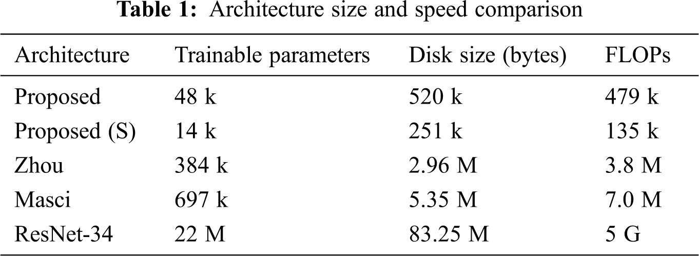
To evaluate the Squeeze Net architecture capacity, we built an even smaller model than the proposed one (called here Proposed (S)). This model uses half the number of filters on the fire and convolution layers.
From Tab. 1, one can see that the proposed architectures are about 10 to 20 times smaller and up to 50 times faster than the ones presented by Zhou et al. [14] and Masci et al. [12]. When compared to traditional state-of-the-art image recognition networks such as ResNet-34, the size of the tested models is significantly smaller. One can see that the proposed model used about 500 times less trainable parameters and about 10,000 times less floating point operations (FLOP) than ResNet-34.
In addition, the size of the proposed model could be reduced even further using Deep Compression (DC) technique [27]. Even though it is shown that DC can reduce the size of models up to 10 times with less than 1% accuracy loss, this test is out of the scope of the present work.
Using the test set (100 samples of each defect), the mean accuracy rate across all predictions for the multiclass classification task is evaluated. This accuracy is calculated by summing the number of right classifications divided by the total number of samples (600). For reference, by random guessing one would expect to achieve an accuracy of 1/6. Fig. 4 compares the result obtained for the studied architectures (Masci, Zhou and Proposed). The thin lines represent each one of the 10 independent training runs. The smooth bold line is constructed using locally weighted scatterplot smoothing (LOESS) regression of all 10 runs.
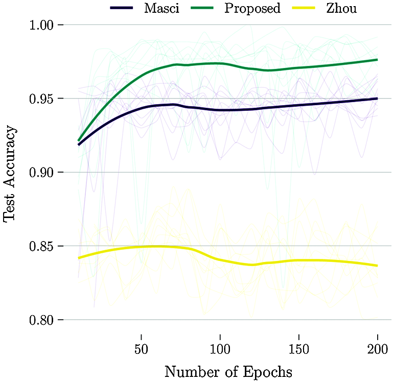
Figure 4: Performance tests comparison of the investigated architectures
The proposed model has overall higher accuracy, and the Zhou’s model [14] the lower one. The authors believe this is due to the choice of the linear activation functions. Even though it is reported by Zhou et al. [14] that the linear activation functions outperformed the rectified ones (ReLu), this finding is contradictory to the literature [28–30]. To verify this issue, a modified version of Zhou’s model with ReLu is investigated. The results are shown in Fig. 5.
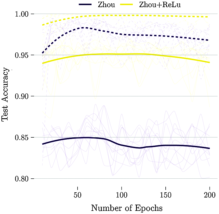
Figure 5: Comparison of train (dashed) and test (solid) performance of Zhou’s architecture against the same architecture with ReLu
Fig. 5 shows clearly that given the same architecture, the usage of ReLu activation functions results in significantly higher accuracy (85% to 95% of test set). This finding is in line with what is observed in most of the literature.
To investigate if we could reduce even further the computational cost of the predictions, the small version (S) of the proposed model is tested. Fig. 6 compares the two versions (original and small size) of the proposed architecture. Also, to evaluate overfitting, train and test performance are shown with dashed and solid lines, respectively. From the figure, no overfitting is noted. Although the performance of the small architecture is good, the larger version outperforms it on all epochs. However, for applications with severely limited memory space or computational power, the small model still manages to classify the defects with above 97% accuracy.
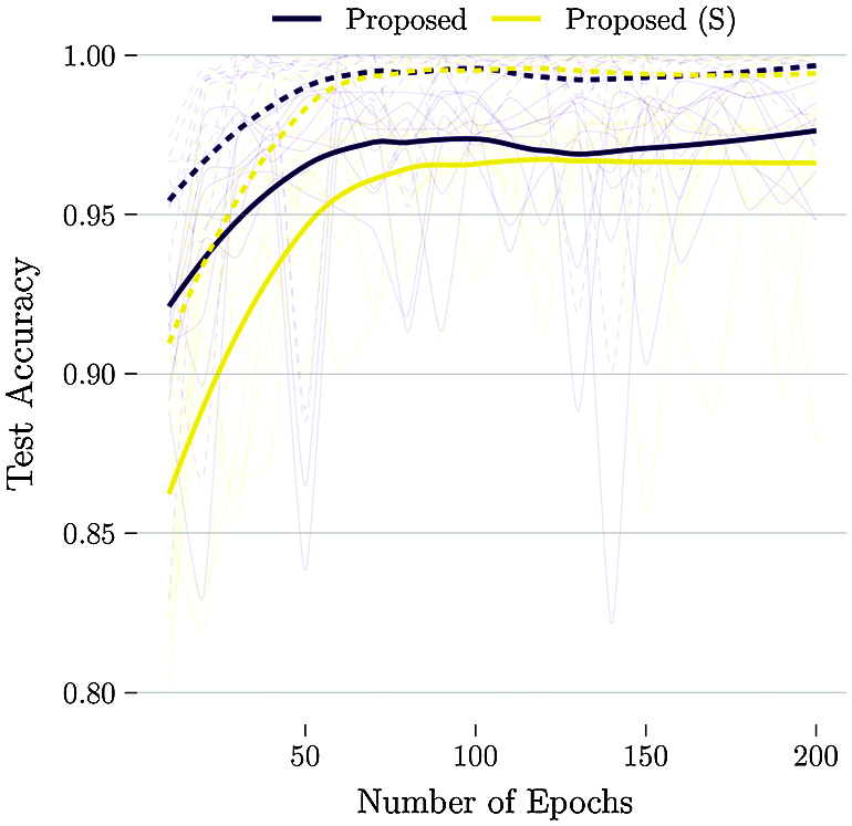
Figure 6: Comparison of train (dashed) and test (solid) performances of the two proposed architectures
For a more reliable way of comparison, the data accuracies are also shown in Tab. 2. The mean accuracy at every 10 epochs is shown. Also, within parentheses, the uncertainty of the last digits is shown. For example, 0.898 (65) means 0.898 ± 0.065 and 0.946 (9) means 0.946 ± 0.009.
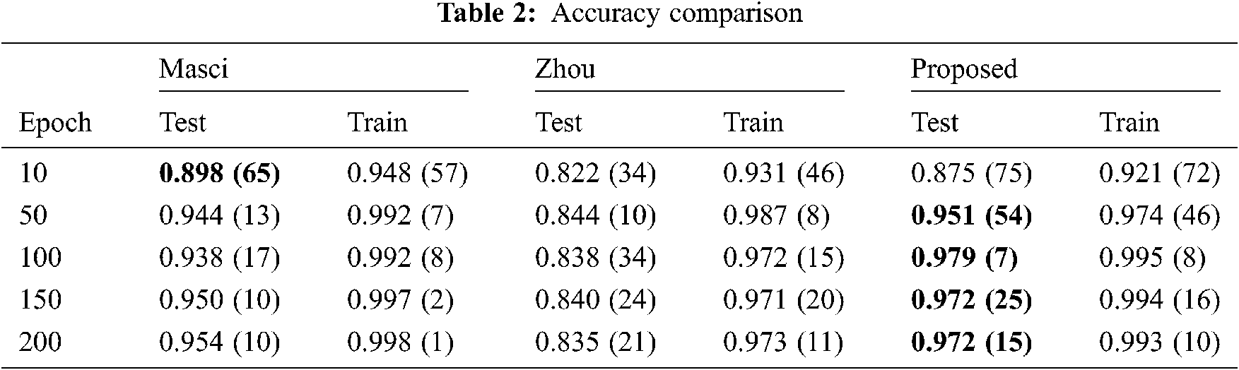
It was observed a performance difference between the Masci’s model presented in the original paper [12] and the one calculated here. In the original paper the authors reported an accuracy of 0.92 (1), but in the present work an accuracy of 0.95 (1) was achieved for the same dataset. We believe this improvement is not by chance and is mainly due to the use of a more modern weight initialization and optimization schemes.
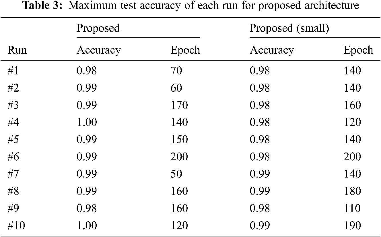
If more data were available, one could use a validation set to early-stop the training procedure. If that is the case an accuracy of over 98% to 100% could be achieved by the proposed model. Tab. 3 shows the best results obtained at each run and the respective epoch it happened. Note that since the models were only saved at each 10 epochs, it is very likely that better models than the ones saved were lost. So, the authors believe that all runs could have achieved near-perfect test accuracy. Also, the results show that using a smaller model causes negligible accuracy loss. However, the results also suggest that the smaller models take more epochs to train, so increasing the number of maximum epochs could yield in better accuracy.
• Usually, industrial computers (installed in a production line) lack performance in favor of robustness. In this context, a reduction of 10 to 20 times of memory usage and 50 times of processing needs could be significant for real-time measurement.
• The employment of state-of-the-art algorithms improved the accuracy obtained by the Masci’s model [12] from 0.92 (1) to 0.95 (1). This is an average error reduction of around 37% (from 8% to 5%).
• The present paper could not reproduce the accuracy reported by Zhou et al. [14] using linear activation function. However, when using ReLu activation, the results are compatible with the reported ones.
• The proposed smart deep convolutional neural network for real-time surface inspection was shown to be more accurate and less computer demanding when compared to other networks designed for the same task.
• Using a state-of-the-art deep neural network such as ResNet-34, the obtained accuracy was over 99.99%. However, the focus of the present work is to provide cheaper-to-evaluate solutions that could be computed in real time without using machines with GPUs.
Funding Statement: The author received no specific funding for this study.
Conflicts of Interest: The authors declare that they have no conflicts of interest to report regarding the present study.
1. T. Piironen, O. Silven, M. Pietikäinen, T. Laitinen and E. Strömmer, “Automated visual inspection of rolled metal surfaces,” Machine Vision and Applications, vol. 3, no. 4, pp. 247–254, 1990. [Google Scholar]
2. D.-M. Tsai and T.- Huang, “Automated surface inspection for statistical textures,” Image and Vision Computing, vol. 21, no. 4, pp. 307–323, 2003. [Google Scholar]
3. L. A. O. Martins, F. L. C. Pádua and P. E. M. Almeida, “Automatic detection of surface defects on rolled steel using computer vision and artificial neural networks,” in Proc. IECON, 2010-36th Annual Conf. on IEEE Industrial Electronics Society, Glendale, AZ, USA, IEEE, pp. 1081–1086, 2010. [Google Scholar]
4. S. Ghorai, A. Mukherjee, M. Gangadaran and P. K. Dutta, “Automatic defect detection on hot-rolled flat steel products,” IEEE Transactions on Instrumentation and Measurement, vol. 62, no. 3, pp. 612–621, 2013. [Google Scholar]
5. K. Song and Y. Yan, “A noise robust method based on completed local binary patterns for hot-rolled steel strip surface defects,” Applied Surface Science, vol. 285, pp. 858–864, 2013. [Google Scholar]
6. R. Ren, T. Hung and K. C. Tan, “A generic deep-learning-based approach for automated surface inspection,” IEEE Transactions on Cybernetics, vol. 48, no. 3, pp. 929–940, 2018. [Google Scholar]
7. C. J. Burges, “A tutorial on support vector machines for pattern recognition,” Data Mining and Knowledge Discovery, vol. 2, no. 2, pp. 121–167, 1998. [Google Scholar]
8. J. Schmidhuber, “Deep learning in neural networks: An overview,” Neural Networks, vol. 61, no. 3, pp. 85–117, 2015. [Google Scholar]
9. Y. LeCun, Y. Bengio and G. Hinton, “Deep learning,” Nature, vol. 521, no. 7553, pp. 436–444, 2015. [Google Scholar]
10. F. Chollet, Deep Learning with Python, 1sted., Shelter Island, New York: Manning Publications Company, 2018. [Google Scholar]
11. F. Chollet and J. J. Allaire, Deep Learning with R, 1sted., Shelter Island, New York: Manning Publications Company, 2018. [Google Scholar]
12. J. Masci, U. Meier, D. Ciresan, J. Schmidhuber and G. Fricout, “Steel defect classification with max-pooling convolutional neural networks,” in Proc. the 2012 Int. Joint Conf. on Neural Networks, Brisbane, Australia, 2012. [Google Scholar]
13. S. Hochreiter, “The vanishing gradient problem during learning recurrent neural net sand problem solutions,” International Journal of Uncertainty, Fuzziness and Knowledge-Based Systems, vol. 6, no. 2, pp. 107–116, 1998. [Google Scholar]
14. S. Zhou, Y. Chen, D. Zhang, J. Xie and Y. Zhou, “Classification of surface defects on steel sheet using convolutional neural networks,” Materiali in Tehnologije, vol. 51, no. 1, pp. 123–131, 2017. [Google Scholar]
15. J. Donahue, Y. Jia, O. Vinyals, J. Hoffman, N. Zhang et al., “DeCAF: A deep convolutional activation feature for generic visual recognition,” in Proc. the 31st Int. Conf. in Machine Learning (ICML 2014Beijing, China, vol. 32, pp. 647–655, 2014. [Google Scholar]
16. W. Chen, Y. Gao, L. Gao and X. Li, “A new ensemble approach based on deep convolutional neural networks for steel surface defect classification,” Procedia CIRP, vol. 72, no. 7, pp. 1069–1072, 2018. [Google Scholar]
17. K. He, X. Zhang, S. Ren and J. Sun, “Deep residual learning for image recognition,” in Proc. 2016 IEEE Conf. on Computer Vision and Pattern Recognition, Las Vegas, NV, USA, pp. 770–778, 2016. [Google Scholar]
18. S. Zagoruyko and N. Komodakis, “Wide residual networks,” in Proc. the 27th British Machine Vision Conference (BMVC 2016York, UK, pp. 87.1–87.12, 2016. [Google Scholar]
19. R. Ye, C.-S. Pan, M. Chang and Q. Yu, “Intelligent defect classification system based on deep learning,” Advances in Mechanical Engineering, vol. 10, no. 3, pp. 1–7, 2018. [Google Scholar]
20. M. D. Zeiler and R. Fergus, “Visualizing and understanding convolutional networks,” in ECCV, 2014-13th European Conf. on Computer Vision, Zurich, Switzerland, pp. 818–833, 2014. [Google Scholar]
21. F. N. Iandola, S. Han, M. W. Moskewicz, K. Ashraf, W. J. Dally et al., “Squeezenet: Alexnet-level accuracy with 50x fewer parameters and 0.5 mb model size,” 2016. [Online]. Avalilable: https://arxiv.org/abs/1602.07360. [Google Scholar]
22. G. Fu, P. Sun, W. Zhu, J. Yang, Y. Cao et al., “A deep-learning-based approach for fast and robust steel surface defects classification,” Optics and Lasers in Engineering, vol. 121, no. 21, pp. 397–405, 2019. [Google Scholar]
23. J. Deng, W. Dong, R. Socher, L.-J. Li, K. Li et al., “ImageNet: A large-scale hierarchical image database,” in Proc. 2009 IEEE Computer Vision and Pattern Recognition, Miami, Florida, USA, pp. 248–255, 2009. [Google Scholar]
24. X. Glorot and Y. Bengio, “Understanding the difficulty of training deep feed forward neural networks,” in Proc. Thirteenth Int. Conf. on Artificial Intelligence and Statistics, Sardinia, Italy, pp. 249–256, 2010. [Google Scholar]
25. Keras, “Keras-Deep learning for humans,” various accesses in 2020, 2020. [Online]. Available: https://keras.io. [Google Scholar]
26. M. Abadi, A. Agarwal, P. Barham, E. Brevdo, Z. Chen et al., “Tensor Flow: Large-scale machine learning on heterogeneous systems, software available from tensorow.org,” 2015. [Online]. Available: https://www.tensorflow.org. [Google Scholar]
27. S. Han, H. Mao and W. J. Dally, “Deep compression: Compressing deep Neural networks with pruning, trained quantization and Huffman coding,” Proc. the 4th Int. Conf. on Learing Representations (ICLR 2016San Juan, Puerto Rico, 2016. [Google Scholar]
28. G. E. Dahl, T. N. Sainath and G. E. Hinton, “Improving deep neural networks for LVCSR using rectified linear units and dropout,” in Proc. 38th IEEE Int. Conf. on Acoustics, Speech, and Signal Processing, Vancouver, Canada, pp. 8609–8613, 2013. [Google Scholar]
29. M. D. Zeiler, M. Ranzato, R. Monga, M. Mao, K. Yang et al., “On rectified linear units for speech processing,” in Proc. 38th IEEE Int.Conf. on Acoustics, Speech, and Signal Processing, Vancouver, Canada, pp. 3517–3521, 2013. [Google Scholar]
30. A. L. Maas, A. Y. Hannun and A. Y. Ng, “Rectifier nonlinearities improve neural network acoustic models,” in Proc. the 30th Int. Conf. on Machine Learning, Atlanta, USA, vol. 30, 2013. [Google Scholar]
 | This work is licensed under a Creative Commons Attribution 4.0 International License, which permits unrestricted use, distribution, and reproduction in any medium, provided the original work is properly cited. |