Computer Systems Science & Engineering DOI:10.32604/csse.2022.018301
Article

A New Random Forest Applied to Heavy Metal Risk Assessment

Ziyan Yu1, Cong Zhang1,*, Naixue Xiong2 and Fang Chen1

1Wuhan Polytechnic University, Department of Mathematics and Computer Science, Wuhan, 430023, China
2Northeastern State University, Department of Mathematics and Computer Science, Tahlequah, OK, 74464, USA
*Corresponding Author: Cong Zhang. Email: hb_wh_zc@163.com
Received: 04 March 2021; Accepted: 30 April 2021

Abstract: As soil heavy metal pollution is increasing year by year, the risk assessment of soil heavy metal pollution is gradually gaining attention. Soil heavy metal datasets are usually imbalanced datasets in which most of the samples are safe samples that are not contaminated with heavy metals. Random Forest (RF) has strong generalization ability and is not easy to overfit. In this paper, we improve the Bagging algorithm and simple voting method of RF. A W-RF algorithm based on adaptive Bagging and weighted voting is proposed to improve the classification performance of RF on imbalanced datasets. Adaptive Bagging enables trees in RF to learn information from the positive samples, and weighted voting method enables trees with superior performance to have higher voting weights. Experiments were conducted using G-mean, recall and F1-score to set weights, and the results obtained were better than RF. Risk assessment experiments were conducted using W-RF on the heavy metal dataset from agricultural fields around Wuhan. The experimental results show that the RW-RF algorithm, which use recall to calculate the classifier weights, has the best classification performance. At the end of this paper, we optimized the hyperparameters of the RW-RF algorithm by a Bayesian optimization algorithm. We use G-mean as the objective function to obtain the optimal hyperparameter combination within the number of iterations.

Keywords: Random forest; imbalanced data; Bayesian optimization; risk assessment

1  Introduction

The accumulation of heavy metals in agricultural land will not only affect the quality of crops, but also the quality of life of the surrounding residents. Soil is a non-renewable resource, and monitoring heavy metal content in soil and conducting risk assessment is a very important part of land management work. Soil heavy metal contamination risk assessment is similar to credit assessment and disease detection in that it involves identifying hazardous samples from a large number of samples. Because relying on domain experts for this work yields inefficient and not entirely reliable results, many scholars have resorted to machine learning techniques to improve efficiency. We propose to apply RF to soil heavy metal contamination risk assessment. RF was first proposed by Breiman in 2001 [1], an integrated learning method based on the Bagging algorithm [2]. RF has been applied in various industries, such as Rodriguez-Galiano et al. [3] who applied RF to land cover classification. Feng et al. [4] used RF extracts inundated regions in the spectral-texture feature space and performs well in urban inundation mapping. RF can also be applied to problems such as outlier detection [5]. Because the sample set and feature set of the input base learner are different and the correlation between the base learners is low, RF has a strong generalization capability.

Although RF performs well on most classification or regression problems, its hyperparameters are always a challenge to tune. Hyperparameters are parameters in a model that are used to define model properties or define the model training process, such as the learning rate in a neural network model. When the learning rate is small, the convergence rate may be too slow and the time cost may increase. A high learning rate can lead to poor results. Bayesian optimization (BO) [6] can handle optimization problems with black-box functions, so it is widely used for hyperparameter tuning of integrated learning methods. At the end of this paper, we performed hyperparameter tuning of the RF using BO.

The rest of this paper is organized as follows: In Sections 2 and 3 describe the RF and Bayes Optimization algorithm. Section 4 present the principles and steps of the W-RF. While the analysis of experiments and obtained results are provided in Section 5. We conclude with final remarks in Section 6.

2  Random Forest

2.1 Bagging

Breiman [7] proposed the Bagging algorithm in 1996. The algorithm is based on Bootstrap implementing replacement sampling on the dataset to get several subsets, and use these subsets to learn several base learners, and finally output the result by voting method or averaging method. For weak learning algorithms, Bagging can improve the prediction accuracy, but it has no significant effect for strong learning algorithms and sometimes even decreases the accuracy of prediction. In 2003, Brylla et al. [8] proposed Attribute Bagging and demonstrated that applying it to a base learner sensitive to attribute increase or decrease can improve the accuracy of the model. In 2009, Paleologo et al. [9] proposed a subagging method for the high imbalance of credit assessment dataset and experimentally confirmed that this subagging can improve the performance of the base classifier.

2.2 RSM and CART Decision Tree

Random Subspace Method (RSM) [10] is a classification algorithm proposed by Ho in 1998. RSM implements random sampling of the feature set to obtain several feature subsets, and trains several base classifiers through the feature subsets. Finally, the classification results are output by voting method.

Classification regression tree (CART) [11] can deal with both classification and regression problems. If the goal is to generate a regression tree, the feature with the smallest squared error value is selected as the splitting node in the CART partitioning process. If the goal is to generate a classification tree, the feature with the smallest Gini index is selected as the segmentation node in the CART partitioning process.

2.3 RF for Classification

When using RF for classification, the number of trees in the forest needs to be defined. Suppose the training set contains n input features. RF performs replacement sampling on the training set to obtain T sub-training sets, and then generates T trees using the sub-training sets. To construct the decision tree, m features are randomly selected from the feature set of the sub-training set using the random subspace method. The optimal feature from the m features is selected as the split node using the minimum Gini index as the division criterion. Finally, RF integrates the classification results of all decision trees by the simple voting method and output them.

Suppose the category space of the dataset is ωj={ω1,...,ωc} , c is the number of categories, hi(x) represents the i -th base classifier, the number of base classifiers is T , and H(x) is the classification result of RF. The classification function of the base classifier is Eq. (1):

vi,j={1,ifhi(x)=ωj0,else (1)

Simple voting methods include majority voting and plurality voting. Majority voting [12] means that when the number of votes for a category exceeds more than half of the number of base classifiers, the category is output as the classification result. If there is no category with more than half of the votes, the classification is rejected.

H(x)={ωj,if∑i=1T⁡vi,j>12∑k=1c⁡∑i=1T⁡vi,kreject,else (2)

where vi,j represents the number of votes obtained by category ωj .

Plurality voting [12] means that the category with the highest number of votes is used as the classification result, without considering whether the number of votes exceeds half of the number of base classifiers. If more than one category receives the highest number of votes, one of the categories is randomly selected for output.

H(x)=ωargmaxj⁡∑i=1T⁡vi,j (3)

where vi,j represents the number of votes obtained by category ωj .

3  Bayesian Optimization

BO is a model-based sequential optimization algorithm (SMBO). Its iterative approach is to complete the first evaluation, then find the next evaluation point for the second evaluation, and so on. When using BO for hyperparametric optimization, the objective function needs to be given as f(x) . If f(x) represents the generalization error of the machine learning model, then according to the objective function, the optimization problem to be solved can be expressed as follows.

x′=argminx∈X⁡f(x) (4)

X is the given hyperparameter search space; x′ is a certain combination of hyperparameters in the hyperparameter search space that minimizes f(x) ; f(x) is the objective function. The objective function can be the generalization error of the model, or the mean square error or accuracy, etc.

The process of BO implementation is:

a. Randomly collect a number of points from the hyperparametric search space and construct a dataset based on the values of the objective function corresponding to these points.

b. Select a probability model to proxy the distribution of this dataset over the objective function. The evaluation point for the next iteration can be determined from the probability distribution. A Gaussian process (GP) is usually used as a probabilistic surrogate model.

c. The next evaluation point is found by maximizing the acquisition function.

d. Combine the evaluation points and corresponding objective function values with the previously constructed dataset, update the probabilistic surrogate model and repeat the above steps. Stop the optimization when the preset number of iterations is reached.

In this way, the minimum of the complex nonconvex objective function can be found with fewer evaluation steps, but more computations are required at each step to determine the next sampling point. The probabilistic surrogate model and acquisition function are the two most important parts of BO. It is called BO because the Bayesian formulas are required in the optimization process. The Bayesian formula is as follows.

p(f|D)=p(D|f)p(f)p(D) (5)

f is the objective function; D={(x1,y1),(x2,y2),...,(xn,yn)} is the dataset consisting of the evaluation point xi and the corresponding objective function value yi=f(xi) , i=1,2,…,n ; p(D|f) is the likelihood distribution of y ; p(f) is the prior probability distribution of f ; p(D) is the marginal likelihood distribution; p(f|D) is the posterior probability distribution of objective function f. The posterior probability distribution describes the confidence level of the unknown objective function [13], after correcting the prior by the observed dataset.

4  Improved Random Forest

Although RF has good classification performance because of the increased sample perturbation by Bagging, it still suffers from the following shortcomings.

a. When there is a class imbalance problem in the input training set, the sub-training set obtained by the Bagging algorithm may contain few or no positive samples. This may lead to under-learning of positive samples by RF.

b. Regardless of the good or bad classification performance of the base classifier, the simple voting method gives all base classifiers equal voting weights, which limits the classification performance of RF.

4.1 Adaptive Bagging

Chen et al. [14] proposed Balanced Random Forest (BRF) and Weighted Random Forest (WRF) to deal with imbalanced data. BRF [14] use stratified bootstrap and down-sampling method to learn imbalanced data. Although down-sampling of negative samples results in the same class priority, it reduces the information that can be learned for each tree in the RF. WRF [14] calculates the Gini index and voting results based on the weights of classes, giving higher weights to positive samples. However, if the weights are not appropriate, the classification results will be greatly affected. To overcome the above problems, an adaptive Bagging algorithm is proposed in this paper. The steps for implementing the adaptive Bagging algorithm are as follows.

a. Calculate pos_num , the number of positive samples in the input training set. Calculate ratio , the percentage of positive samples in the total samples.

b. Draw bootstrap samples from the input training data set to build a sub-training set.

c. If the ratio is less than 0.1, go to step 4, otherwise go to step 5.

d. Calculate the number of positive samples in the sub-training set. If the number is less than pos_num , bootstrap sampling is performed on the positive samples in the input training set so that the number of sub-training sets is equal to pos_num .

e. Generating base classifiers using sub-training sets.

Adaptive Bagging does not limit the number of positive samples in each sub-training set, but ensures that each base classifier can learn a certain number of positive sample information.

4.2 Weighted Voting

The second deficiency of RF can be improved by changing the simple voting method to a weighted voting method. Higher weights are assigned to base classifiers with better classification performance and lower weights are assigned to base classifiers with poorer classification performance. Currently, many scholars have demonstrated that the weighted voting method can improve the classification performance of RF. For example, Yan et al. [15] derived error rate bounds for the confidence voting method and introduced a new weight assignment method to improve the classification accuracy of the algorithm. Zhang et al. [16] uses the posterior probability of the Bayesian equation to express the credibility. The larger the value of posterior probability, the higher the credibility of the base classifier and the larger the weight. He [17], based on Zhang et al. [16], proposed to use the out-of-bag (OOB) accuracy of RF instead of the posterior probability value as the credibility, and obtained a new voting weight calculation formula. It improves the classification accuracy of RF and reduces the computational complexity.

In this paper, we propose to assign weights based on the classification performance metrics of the tree in RF. The metrics for classification performance include accuracy, precision, recall, F1-score, G-mean, etc. In order to select the most suitable metric to be used for weighted voting, we conducted experiments under different metrics. The selected metrics are G-mean, F1-score and recall. Eq. (6) shows the weight function.

weight(i)=metric(i)∑i=1T⁡metric(i) (6)

T is the number of base classifiers; metric(i) is the performance metric of the i base classifier. When the metric is G-mean, it is called G-mean weighted Random Forest (GW-RF). When the metric is F1-score, it is called F1-score weighted Random Forest (FW-RF). When the metric is recall, it is called recall weighted Random Forest (RW-RF).

This paper studies the binary classification problem, Eq. (7) shows the voting function:

H(x)=sign(∑i=1T⁡weight(i)hi(x)) (7)

weight(i) is the weight of the i base classifier; sign(x)={1,x≥0−1,x<0 .

4.3 W-RF Algorithm

In binary classification problems such as risk assessment and disease diagnosis, the input datasets are usually imbalanced datasets with less than 10% of the total number of positive samples. The W-RF algorithm uses adaptive Bagging and weighted voting methods to better learn imbalanced data. The pseudo-code of the W-RF algorithm is described below.

Algorithm 1. W-RF

Input: training data set S ; test data set D ; y={−1,1} ; the number of features d ; the number of CART trees T .

Output: Classification result H(x)

1: for i = 1, 2, …, T do

2: calculate the number of positive samples pos_num in S and atio .

3: draw bootstrap samples from S to build a sub-training set Si .

4: if ratio≤0.1 , then go to step 4; else go to step 5.

5: calculate the number of positive samples pos_numi in Si .

6: if pos_numi<pos_num , then do bootstrap sample again for the positive samples in S , so that pos_numi=pos_num .

7: randomly extract k(k≤d) features from Si to form a feature subset Si′ .

8: use Si′ to train a base classifier hi(x) .

9: end for

10: combine h1(x),h2(x),...,hi(x) to ensemble classifier E={h1(x),...hi(x)}

11: use test data set D to calculate the metric(i) of each base tree, and use metric(i) to calculate weight(i) with Eq. (6).

weight(i)=metric(i)∑i=1T⁡metric(i) (6)

12: use Eq. (7) to calculate the final classification result.

H(x)=sign(∑i=1T⁡weight(i)hi(x)) (7)

5  Experiments

5.1 Dataset

The dataset 1,2 shown in the Tab. 1 are downloaded from the OODS library [18]. The Cardio dataset is a fetal electrocardiogram dataset edited by a professional obstetrician, with 176 positive samples and 1655 negative samples. The Ionosphere dataset is an ionospheric dataset with two categories, good and bad. Good category has 225 samples and bad category has 126 samples. The Diabetes dataset is downloaded from the UCI machine learning repository [19]. It has 268 positive samples and 500 negative samples.

The Heavy metal dataset comes from Wuhan Academy of Agricultural Sciences, which contains sampling information and measurement results of eight heavy metals (As, Cd, Cr, Cu, Ni, Pb, Zn, Hg) in agricultural soils around Wuhan. The dataset contains 12 variables: farmland type, altitude, longitude, latitude, and the content of the heavy metals. It has 87 positive samples and 1074 negative samples.

5.2 Performance Measurement

In order to evaluate the performance of RF, the paper use metrics such as classification accuracy, precision, recall, F1-score, and G-mean. All these metrics are calculated through a confusion matrix. The calculation formula is shown in Eqs. (8)–(12). Tab. 2 shows the confusion matrix. In addition to the above metrics, the receiver operating characteristic (ROC) curve and the area under the ROC curve (AUC) are also used.

Accuracy=TP+TNP+N (8)

Precision=TPTP+FP (9)

Recall=TPTP+FN (10)

F1−socre=2×Precision×RecallPrecision+Recall (11)

G−mean=TPTP+FN×TNTN+FP (12)

5.3 Performance Comparison

Use the 5-fold cross-validation method for experiments. The experimental dataset is divided into five sub-data sets. Given that the original dataset is D , the five sub-datasets are D1 , D2 , D3 , D4 , D5 . In each training, Di is selected from the five subsets as the test set, and the other four subsets are combined as the training set, and i=1,2,...,5 . Take the average of accuracy, precision, recall, F1-score and G-mean obtained from 5 training sessions, draw the corresponding ROC curve and calculate the AUC value.

5.3.1 Performance Comparison between W-RF and RF

Tab. 3 compares the performance of different algorithms on the Cardio dataset. It can be observed that in addition to precision, the results of GW-RF are the best on other metrics. Fig. 1 shows the ROC curve and AUC value of the Cardio dataset. For five subsets, comparing the AUC values under several algorithms shows that the AUC values under W-RF are mostly higher than RF.

Figure 1: ROC curve and AUC value of the Cardio dataset

Tab. 4 compares the performance of different algorithms on the Ionosphere dataset. It can be observed that the metrics results of GW-RF are best. Fig. 2 shows the ROC curve and AUC value of the Ionosphere dataset. It can be found that on the ionospheric dataset 4, the AUC value obtained by the W-RF algorithm is not ideal. But in other subsets, the AUC values obtained are all higher than RF.

Figure 2: ROC curve of the Ionosphere dataset

Tab. 5 shows the performance of different algorithms on the Diabetes dataset. Fig. 3 shows the ROC curve and AUC value of the Diabetes dataset. As can be seen from Tab. 5, the results of RW-RF are the best in most of metrics. Comparing the AUC values of these algorithms, the AUC value of W-RF is mostly higher than that of RF. Analyzing the experimental results, we can conclude that the classification performance of W-RF is better than that of RF in most cases.

Figure 3: ROC curve of the diabetes dataset

5.3.2 Comparison of Risk Assessment Performance

To verify the effectiveness of the W-RF algorithm, the algorithm was compared with RF, K-nearest neighbors (KNN), logistic regression (LR) and support vector machine (SVM) [20] on the heavy metal dataset. The learning rate of LR is set to 0.1, and the number of iterations is set to 500. The number of K nearest neighbor samples of the KNN is set to 5. SVM use the polynomial kernel as the kernel function, and the penalty coefficient C is set to 1. The number of trees for RF and W-RF is set to 50, and the others remain the default.

Tab. 6 compares the performance of different algorithms on the heavy metal dataset. Comparing the accuracy, all the algorithms are above 90% except SVM. On the contrary, when comparing recall, all the algorithms except SVM and RW-RF have less than 50% recall. It shows that the partitioned hyperplane of SVM has certain distinguishing ability for positive samples, but has a large classification errors for negative samples. Regardless of whether the weight is set by G mean or F1 score, the five metrics obtained by W-RF in this experiment are better than RF and other algorithms. Fig. 4 shows the ROC curve and AUC value of the Heavy metal dataset. For five subsets, comparing the AUC values under several algorithms shows that the AUC values under RW-RF are mostly higher than other algorithms.

Figure 4: ROC curve of the Heavy metal dataset

5.4 Parameter Optimization

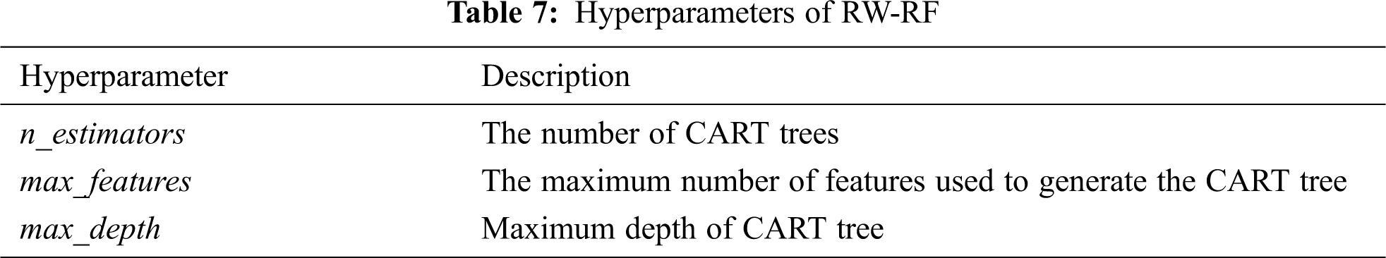
After the experiment in Section 5.3.3, it is found that RW-RF has the best performance on the heavy metal dataset. This section uses the BO to complete the hyperparameter tuning of RW-RF. Tab. 7 shows the hyperparameters of RW-RF.

This paper uses BayesianOptimization function from the bayesian-optimization library [21] to search which hyperparameter combination yields the best performance results. This function uses GP as probabilistic surrogate model, and the acquisition points of the next iteration are obtained by maximizing the confidence interval of GP. We set G-mean as the optimized objective function and define the search space as (n_estimators, max_features, max_depth): the number of CART trees range in the integer interval {50, 150}, and the ranges of max_features and max_depth are also integer interval {1, 12} and {1, 10}.

Fig. 5 shows the change of G-mean in 30 iterations of BO. The G-mean derived at the 29th iteration is the largest, at the time n_estimators=61 , max_features=10 , max_depth=7 , and the G-mean is 0.981.

Figure 5: The change of G-mean in 30 iterations of BO

6  Conclusion and Future Work

Based on the shortcomings of RF in classification performance on imbalanced datasets, this paper proposed a W-RF algorithm combining adaptive Bagging and weighted voting. Adaptive Bagging first calculates the proportions of different types of samples on the input training set, and judges whether the current training set is an imbalanced dataset. Secondly, if it is an imbalanced dataset, calculate the number of positive samples in the sub-training set and compare it with the number before sampling. If the number is less than before, sample the positive samples with replacement again to keep the positive samples at least a certain proportion in the sub-training set. The weighted voting method is to give higher weights to the base classifier with higher performance metrics. The performance metrics we choose includes G-mean, F1-score, and recall.

From the experiments on various datasets, we can conclude that the performance of GW-RF, RW-RF, and FW-RF are better than RF and other classification algorithms. However, we could not determine which of GW-RF, RW-RF or FW-RF is better. For heavy metal risk assessment, RW-RF has the best classification performance. Therefore, we use RW-RF to conduct risk assessment experiments on heavy metal pollution in agricultural fields around Wuhan and obtained the optimal combination of hyperparameters using BO. In future work, consider using deep reinforcement learning methods [22] for heavy metal pollution risk assessment, or study images of heavy metal pollution distribution, and try to make image predictions [23]. In addition, since this paper only studies the binary classification problem, we will consider extending the binary classification problem to the multi-classification problem.

Funding Statement: This work was supported in part by the Major Technical Innovation Projects of Hubei Province under Grant 2018ABA099, in part by the National Science Fund for Youth of Hubei Province of China under Grant 2018CFB408, in part by the Natural Science Foundation of Hubei Province of China under Grant 2015CFA061, in part by the National Nature Science Foundation of China under Grant 61272278, and in part by Research on Key Technologies of Intelligent Decision-making for Food Big Data under Grant 2018A01038.

Conflicts of Interest: The authors declare that they have no conflicts of interest to report regarding the present study.

This work is licensed under a Creative Commons Attribution 4.0 International License, which permits unrestricted use, distribution, and reproduction in any medium, provided the original work is properly cited.