Computer Systems Science & Engineering DOI:10.32604/csse.2022.018219
Article

Efficient Process Monitoring Under General Weibull Distribution

Saman Hanif Shahbaz and Muhammad Qaiser Shahbaz*

Department of Statistics, King Abdulaziz University, Jeddah, Kingdom of Saudi Arabia
*Corresponding Author: Muhammad Qaiser Shahbaz. Email: mkmohamad@kau.edu.sa
Received: 01 March 2021; Accepted: 29 April 2021

Abstract: Product testing is a key ingredient in maintaining the quality of a production process. The production process is considered an efficient process if it is capable of quick identification of faulty products. The items produced by any production process are usually packed and acceptance or rejection of the pack depends upon its conformity to some specified quality level. Generally, the specified quality level is based upon the number of defective items found in the inspected number of items. Such decisions are based upon some rules and usually acceptance of the pack is based upon a fewer number of defective items in the pack. Such questions can be answered by using acceptance sampling plans. The acceptance sampling plans assume the fact that the quality level of the item follows some probability distribution. The sampling plans based upon some classical probability distributions are available but often it happens that the quality behavior of the product does not follow a simple probability model and hence the available sampling plans fail. In this paper, we have developed acceptance sampling plans when the product life follows a general Weibull distribution. The sampling plans have been constructed by considering the crisp and fuzzy behavior of the acceptance probability. These sampling plans have been constructed by assuming an infinite lot size. It has been found that the number of items required for inspection decreases with an increase in some parameters.

Keywords: General Weibull distribution; sampling plans; acceptance probability; fuzzy plan

1  Introduction

Product inspection is an important phase in the production process. It is always desired that the produced product meet some specified characteristics. The quality control engineers are vigilant in monitoring the process so that the items which do not meet certain quality level are not shipped to the customers. Continuous monitoring of the lots of products at a production plant is therefore necessary. It is not possible to inspect all the items in a lot and hence a sample of the produced items is inspected and the decision about the lot is made if the number of defective items in sampled items is less than a pre-specified value. The acceptance sampling plan is a useful statistical method that helps the quality control engineer in making such decisions. The acceptance sampling plans have a long history in the field of quality control. The classical use of acceptance sampling plan was introduced by Sobel et al. [1]. The acceptance sampling plans have been extensively discussed by Feigenbaum [2] and Montgomery [3].

The acceptance sampling plans are constructed by specifying an acceptable level for the product. The acceptance sampling plans have been studied by a number of authors assuming that the life length of the product follows some specified probability distribution. Several authors have proposed the sampling plans assuming that the life length of the product has a certain underlying probability distribution. The sampling plans for gamma-distributed product life has been studied by Gupta et al. [4] for different combinations of the parameters. The Weibull distribution has been an area of interest by several authors in the context of acceptance sampling plans. Classical work on use of Weibull distribution in acceptance sampling plans has been done by Goode et al. [5].

Several other authors have used Weibull distribution to develop the sampling plans under different situations. The sampling plans for two parameter Weibull distribution have been discussed by Fertig et al. [6] and another version of the Weibull sampling plans has been discussed by Jun et al. [7]. The repetitive group acceptance sampling plan for Weibull distribution is given by Yan et al. [8]. The sampling plan under progressive type I censoring for Weibull distribution has been discussed by Ding et al. [9], among others. The sampling plan for power Lindley distribution, introduced by Ghitany et al. [10], has been proposed by Hanif Shahbaz et al. [11]. The study of acceptance sampling plans is ever increasing and in this paper we have discussed the acceptance sampling plans when the life length of the product follows the Topp–Leone weighted Weibull distribution, proposed by Abbas et al. [12]. The plan of the paper follows.

In Section 2 we have given a brief about the Topp–Leone weighted Weibull distribution. An overview of the acceptance sampling plans is given in Section 3. In Section 4 we have given the exact sampling plans for Topp–Leone weighted Weibull distribution under infinite lot size followed by the fuzzy sampling plan in Section 6. Section 6 contains some conclusions and recommendations.

2  A General Weibull Distribution

A method of generating weighted distributions has been proposed by Azzalini et al. [13] and is named as the weighted class of distributions. The method has been used by Refs. [14–16] to propose some weighted Weibull distributions. The Topp–Leone family of distributions has been proposed by Al-Shomrani et al. [17] as an alternative to the Beta family of distributions, proposed by Eugene et al. [18]. The Topp–Leone Weighted Weibull, TLWW for short, distribution has been recently proposed by Abbas et al. [12] by using the weighted Weibull distribution in the Topp–Leone family of distributions. The density and distribution functions of the TLWW distribution are

f(x;b,α,γ,λ)=2bαγ(1+λγ)xγ−1e−2αxγ(1+λγ)[1−e−2αxγ(1+λγ)]b−1;x,b,α,γ,λ>0 (1)

and

F(x;b,α,γ,λ)=[1−e−2αxγ(1+λγ)]b. (2)

For the sake of simplicity, we will assume that α=1 and hence the distribution function becomes

F(x;b,α,γ,λ)=[1−e−2xγ(1+λγ)]b. (3)

The expressions of moment and quantile function for TLWW distribution are

μr/=∑j=0∞(−1)jΓ(b+1)j!Γ(b−j)(1j+1)r/γ+1[2−r/γ(1+λγ)−r/γ] (4)

and

Q(p)=−[ln(1−p1/b)2(1+λγ)]1/γ;b,γ,λ>0;0<p<1. (5)

The mean of the distribution is immediately written from Eq. (4) and is

μ=∑j=0∞(−1)jΓ(b+1)j!Γ(b−j)(1j+1)1/γ+1[2−1/γ(1+λγ)−1/γ] .

The mean and quantile function provide the basis for the construction of the sampling plans. In this paper, we have constructed the acceptance sampling plans when the life of a component follows the TLWW distribution.

In the following section, we will briefly discuss the simple and fuzzy acceptance sampling plans.

3  Acceptance Sampling Plan

Acceptance sampling plans have widespread applications in quality control, see for example [3]. These plans are used to accept or reject the lot on the basis of a random sample. The acceptance sampling plans are categorized by the number of items inspected (n) and the maximum allowed number of the defective items (c) for acceptance of the lot. The probability of acceptance of an infinite size lot is given as

L(p)=∑i=0c(ni)pi(1−p)n−i, (6)

where c is the maximum number of allowed defectives in a lot and p is a pre–assigned probability.

The acceptance sampling plans are based on continuing an experiment until a pre–specified time point, t0 , and terminating the experiment after that. The plan suggests accepting the lot if fewer than c defective items are inspected within the interval [0,t0]. The acceptance or rejection of the lot is equivalent to testing the hypothesis H0:μ>μ0 where μ is the average life of the component and μ0 is some pre–specified value. The sampling plans are also based upon two probabilities, namely consumer risk, β , and producer risk, α . The acceptance sampling plan is based upon solving the following two inequalities for n and c

∑i=0c(ni)(AQL)i(1−AQL)n−i≥1−α (7)

and

∑i=0c(ni)(LTPD)i(1−LTPD)n−i≤β (8)

where AQL is the acceptable quality level, and LTPD is the lot tolerance percent defective. Inequalities Eqs. (7) and (8) use binomial distribution since it is assumed that the lot size is infinite or when N>>c∗n ; where N is the lot size and c is a sufficiently large number, say 500 or more. When the lot size is finite, then the binomial distribution is replaced with the hypergeometric distribution.

Often the probabilities are fuzzy and in such cases, we have to adjust the computation of the values of the plan parameters by considering this fuzziness. The suitable change that has to be made is to adjust Eqs. (7) and (8) by replacing the conventional binomial distribution with the neutrosophic binomial distribution which is given by Buckley et al. [19] as

P¯(x)[δ]={(nx)px(1−p)n−x|S} (9)

for 0≤δ≤1 and S is the statement “ p∈p¯[δ]&q∈q¯[δ] ”. It is well known that for a specific fuzzy set P¯(x)[δ]=[Px1(δ),Px2(δ)] is such that Px1(δ)=min{P¯(x)[δ]} and Px2(δ)=max{P¯(x)[δ]} .

The fuzzy acceptance sampling plan is therefore based upon obtaining a pair of values (n,c) for the fuzzy probability P¯[δ] . The sampling plan parameters are therefore obtained by solving

{∑i=0c(ni)(AQL)i(1−AQL)n−i|S}≥1−α (10)

and

{∑i=0c(ni)(LTPD)i(1−LTPD)n−i|S}≤β, (11)

where AQL is now fuzzy acceptable quality level and LTPD is fuzzy lot tolerance percent defective.

We will now discuss the exact and fuzzy sampling plans in the following.

4  Exact Sampling Plan under Topp–Leone Weighted Weibull Distribution

In this section we have discussed the exact sampling plans when the product life follows the TLWW distribution.

4.1 The Sampling Plans

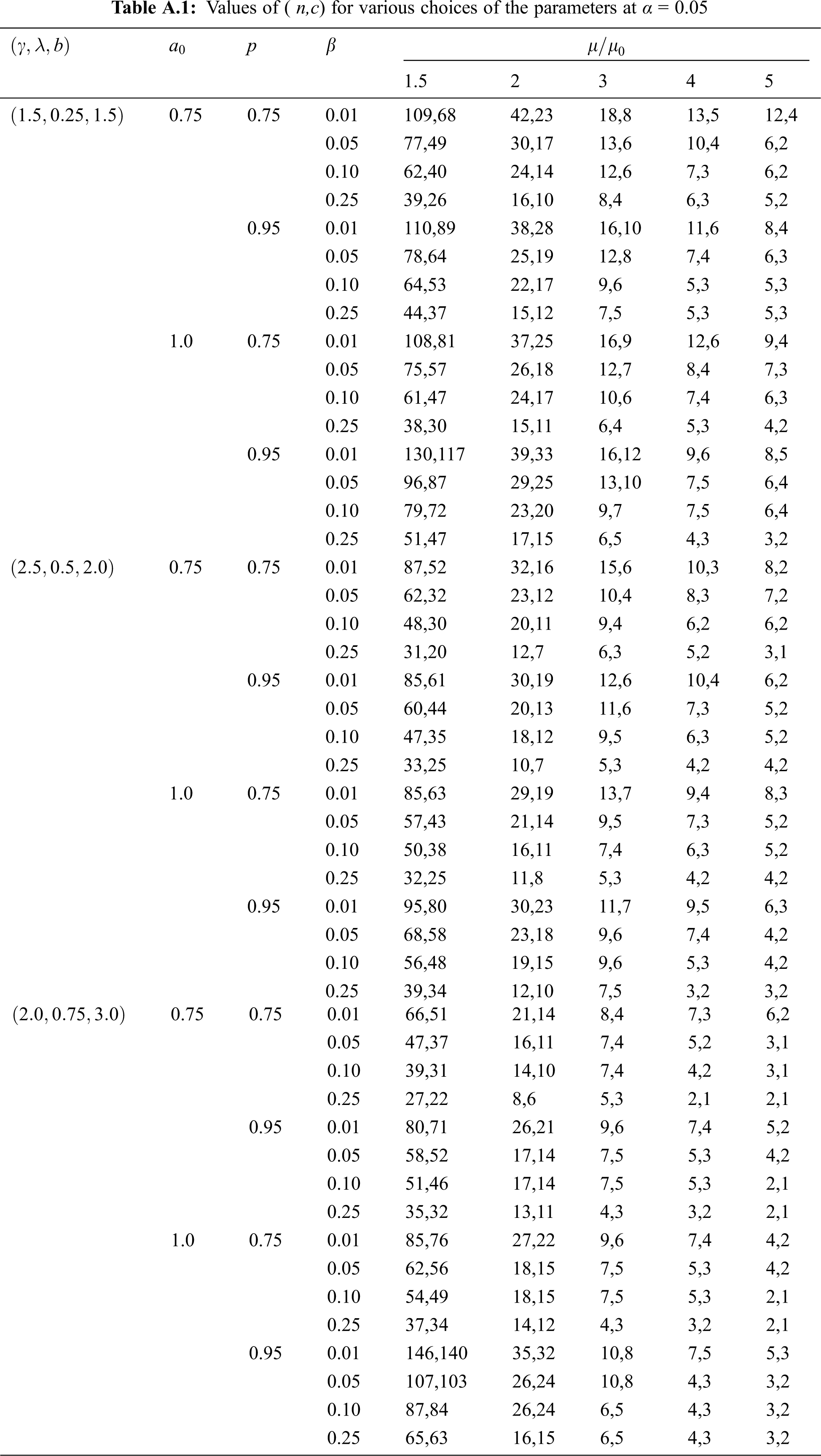
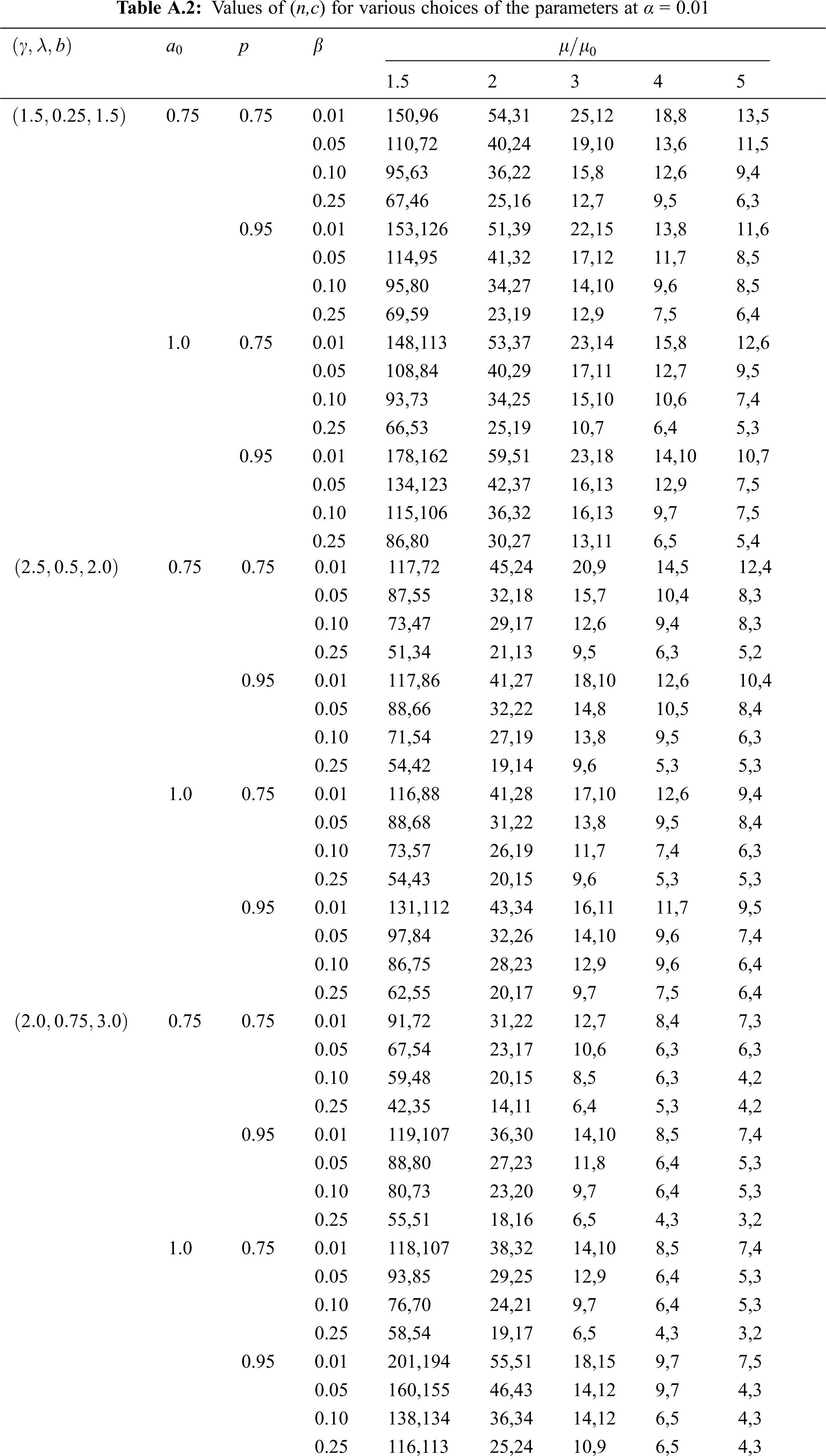
This section contains the exact sampling plan when lot size is infinite and life length of the product follows TLWW distribution. The sampling plan is based upon obtaining the values of n and c which satisfies Eqs. (7) and (8). The quantities AQL and LTPD are obtained from the distribution and quantile function of TLWW distribution given in Eqs. (3) and (5).

Now assuming that the life length of the product is t0=a0μ0 , where μ0 is the average life of the product, and using x=a0μ0=aμ(μ/μμ0−μ0)−1 and further using μ=Q(u) , we can write Eq. (3) as

p=[1−exp⁡{−2a0λQλ(u)(μμ0)−λ(1+λγ)}]b (12)

The acceptance sampling plans are constructed for various ratios of μ/μ0−μ0,γ,λ and b . The values of n and c which satisfy inequalities Eqs. (7) and (8), for different values of α , are given in Table A.1 and Table A.2, respectively, in Appendix A. These values are obtained by assuming μ/μμ0−μ0=1 for LTPD. The values of n and c in these tables provide information about the number of items to be put on the test and the number of defective items observed for rejection of the lot. For example, in Table A.1, the values of n and c for γ=2.5,λ=0.5,b=2.0,a0=0.75,p=0.75,α=0.05,β=0.05 and μ/μμ0−μ0=3 are 12 and 6, respectively. These values indicate that if the quality control engineer is interested in testing the hypothesis that the life length of a component is 1000 hours and the true average life is thrice this value, then the engineer can test 12 items and if fewer than 6 items fail in 750 hours then the engineer can conclude with 95% confidence that the life is more than 3000 hours.

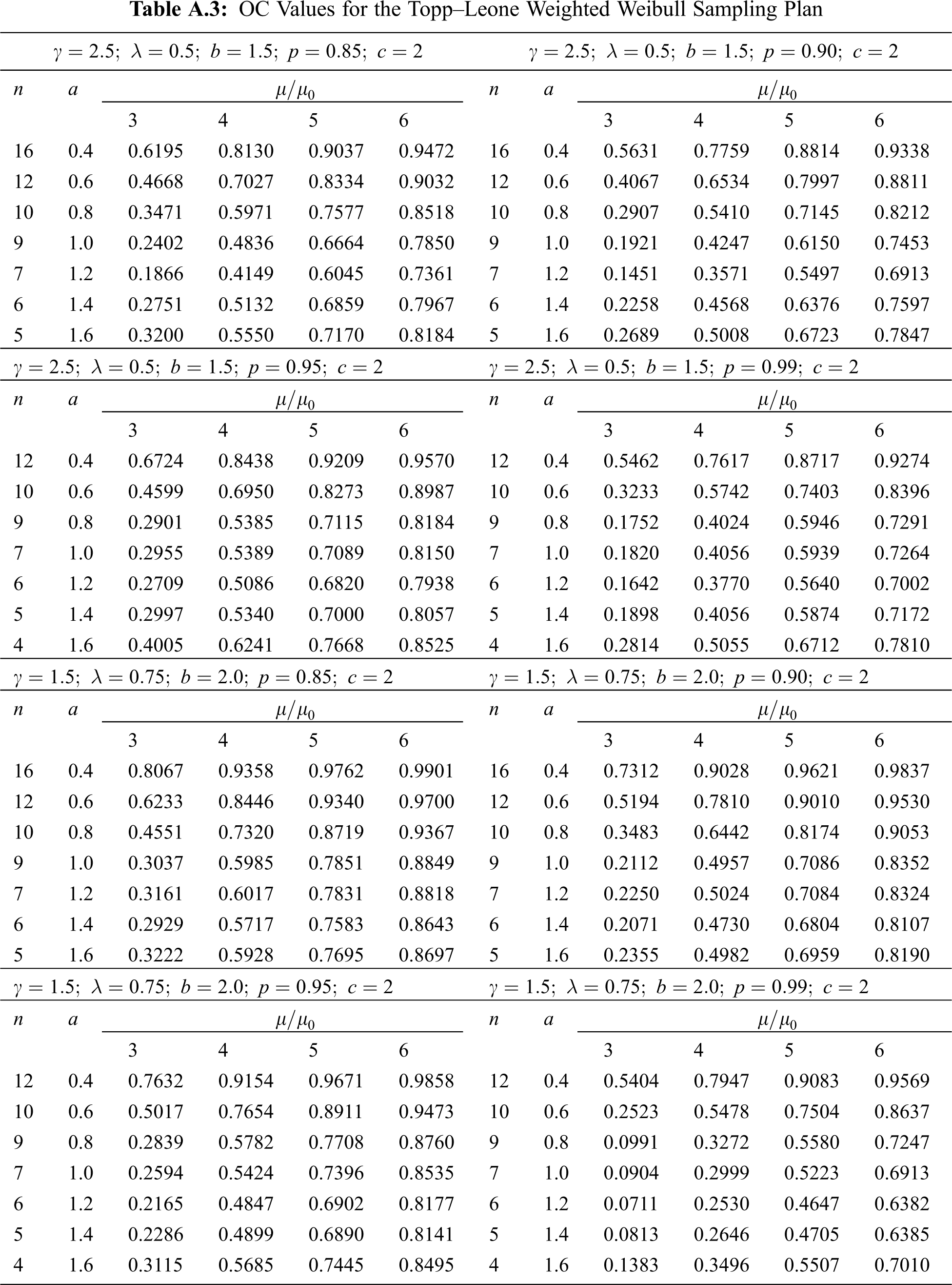
4.2 Operating Characteristic Curve

The operating characteristic (OC) curve is a useful way to decide the performance of an acceptance sampling plan. The OC values for a sampling plan give the probability of acceptance of the lot under a specific sampling plan when the actual lot contains a specified percentage of defective items. The operating characteristic values can be computed by using Eq. (6). The OC values for the given sampling plan under Topp–Leone weighted Weibull distribution with specific values of the parameters are given in Table A.3 in Appendix A. We can see that the probability of acceptance decreases as the value of “a0” increases for the fixed ratio μ/μμ0−μ0 . Additionally, we can see that for a fixed value of “a0”, the acceptance probability increases with an increase in μ/μμ0−μ0 .

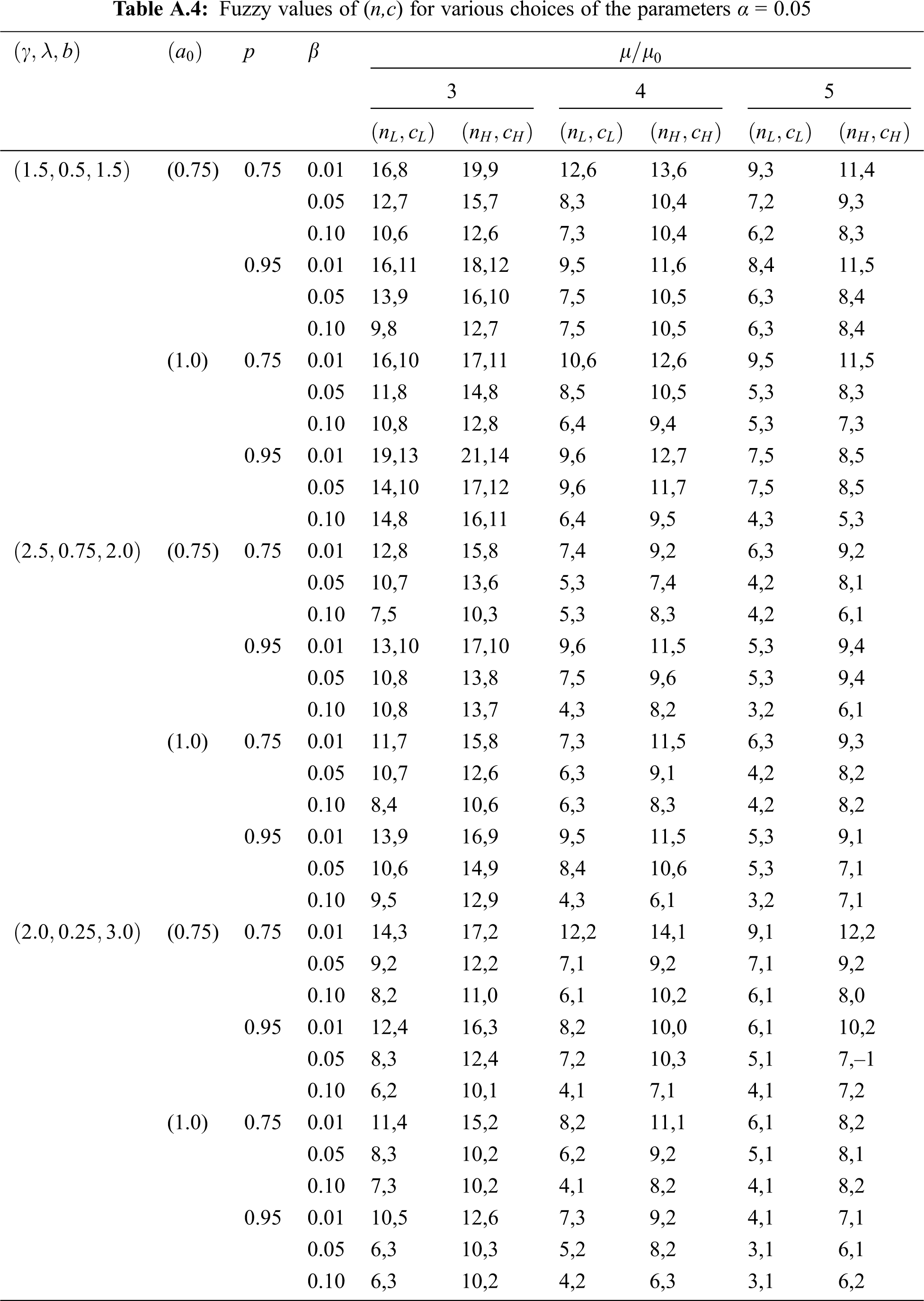
5  Fuzzy Sampling Plans under General Weibull Distribution

The fuzzy sampling plans are an extension of conventional sampling plans and are based upon the fuzzy binomial distribution. In this section we have studied the fuzzy sampling plan when the product life follows the TLWW distribution. The plan parameters are computed by using the fuzzy inequalities given in Eqs. (10) and (11). In the case of a fuzzy sampling plan, the plan parameters are pair of values (nL,cL) and (nH,cH) . These values are computed by assuming the fuzziness of the parameter a0 , which controls the average life of the product. We have used fuzzy values of a0 around 0.75 and 1.0 to obtain the plan parameters. These values are given in Table A.4 in Appendix A. The fuzzy plan parameters now provide an interval for both n and c. For example the plan parameters for γ=1.5,λ=0.5,b=1.5,a0=(0.75),p=0.75,α=0.05,β=0.05 and μ/μμ0−μ0=4 are (8,10) and (3,4) . These values indicate that if the quality control engineer is interested in testing the hypothesis that the life length of a component is 1000 hours and the true average life is four-time of this value, then the engineer can test between (8,10) items and if between (3,4) items fail in (750) hours then the engineer can conclude with 95% confidence that the life is more than 4000 hours.

6  Conclusions

In this paper, we have developed exact and fuzzy sampling plans when the product life follows Topp–Leone weighted Weibull distribution. The sampling plans have been constructed for various choices of the parameters and for various ratios of μ/μμ0−μ0 . These sampling plans have been constructed for infinite lot sizes. We have observed for the exact sampling plan that the number of items required for inspection decreases with an increase in certain parameters.

We have further observed that for the fuzzy sampling plan we have pair of (n,c) as the probability falls within an interval. We have seen that the plan parameters are dependent upon μ/μμ0−μ0 and that the number of items required for inspection decreases with an increase in μ/μμ0−μ0 . This is also true for the values of c. We have also observed that parameter b of Topp–Leone weighted Weibull distribution has a significant effect on the plan parameters. We have observed that the plan parameters and b are inversely related.

Funding Statement: The authors received no specific funding for this study.

Conflicts of Interest: The authors declare that they have no conflicts of interest to report regarding the present study.

Appendix A

This work is licensed under a Creative Commons Attribution 4.0 International License, which permits unrestricted use, distribution, and reproduction in any medium, provided the original work is properly cited.