Computer Systems Science & Engineering DOI:10.32604/csse.2022.018034
Article

An Automated Brain Image Analysis System for Brain Cancer using Shearlets

R. Muthaiyan1,* and Dr M. Malleswaran2

1Department of Electronics and Communication Engineering, University College of Engineering Thirukkuvalai, Tamilnadu, 610204, India
2Department of Electronics and Communication Engineering, University College of Engineering Kancheepuram, Kancheepuram, 631552, India
*Corresponding Author: R. Muthaiyan. Email: muthume2005@gmail.com
Received: 22 February 2021; Accepted: 27 April 2021

Abstract: In this paper, an Automated Brain Image Analysis (ABIA) system that classifies the Magnetic Resonance Imaging (MRI) of human brain is presented. The classification of MRI images into normal or low grade or high grade plays a vital role for the early diagnosis. The Non-Subsampled Shearlet Transform (NSST) that captures more visual information than conventional wavelet transforms is employed for feature extraction. As the feature space of NSST is very high, a statistical t-test is applied to select the dominant directional sub-bands at each level of NSST decomposition based on sub-band energies. A combination of features that includes Gray Level Co-occurrence Matrix (GLCM) based features, Histograms of Positive Shearlet Coefficients (HPSC), and Histograms of Negative Shearlet Coefficients (HNSC) are estimated. The combined feature set is utilized in the classification phase where a hybrid approach is designed with three classifiers; k-Nearest Neighbor (kNN), Naive Bayes (NB) and Support Vector Machine (SVM) classifiers. The output of individual trained classifiers for a testing input is hybridized to take a final decision. The quantitative results of ABIA system on Repository of Molecular Brain Neoplasia Data (REMBRANDT) database show the overall improved performance in comparison with a single classifier model with accuracy of 99% for normal/abnormal classification and 98% for low and high risk classification.

Keywords: Brain image analysis; wavelets; Shearlet; multi-scale analysis; hybrid classification

1  Introduction

The brain is the primary organ of the human body. As the cause of brain cancer is still unknown, an early diagnosis is required to decrease the mortality rate. Image classification is one of the diagnostic approaches used in the medical field which does not require segmentation [1–3]. Most of the image classification algorithms fall into one of the two categories; supervised and unsupervised. The former one learns the inherent patterns of training data for the classification using neural networks [4–6], Support Vector Machine (SVM) [7–11], k-Nearest Neighbor (kNN) [12], Naive Bayes (NB) [13] whereas the later one depends only on the input data. The clustering approach such as k-means and fuzzy-c-means come under unsupervised categories. When compared to unsupervised systems, the supervised systems give better results as they learn or trained from many samples.

A regularized extreme learning machine is discussed in Gumaei et al. [4] which combines two feature extraction approaches; normalized gist with Principal Component Analysis (PCA). These features help to classify brain tumor using a feed forward neural network. A convolutional neural network structure is used for feature extraction and classification in Sultan et al. [5]. It consists of 16 layers in which the features are selected in convolution and rectified linear unit. The dropout layer is used to prevent over fitting. Then, the fully connected layer and softmax layer is used for classification. Another deep learning approach is described in Kumar et al. [6] which use Discrete Wavelet Transform (DWT) to decompose the input images and the obtained feature space is reduced by auto-encoder.

Though deep learning approaches provide better results, it is very difficult to understand their architectures and also time complexity is very high. To achieve highest accuracy with reduced complexity, a hybrid approach is developed in this study using three different classifiers; kNN, NB and SVM. It is well known that the hybrid approach combines the qualities of each technique and thus provides better performance than single approach.

An approach to classify brain MRI images is described in Madheswaran et al. [7]. The input brain images are decomposed by DWT and the features are extracted by genetic algorithm. The parameters like, smoothness, entropy, correlation, root mean square and kurtosis are analyzed. SVM classifier is used for the classification. MRI brain image classification using SVM with various kernels is described in Mallick et al. [8]. Fuzzy-c-means algorithm is used to remove the skull region. Then, GLCM features are extracted and then irrelevant features are eliminated using genetic algorithm with joint entropy. SVM classifier is used for classification.

The energy features of different wavelet families are discussed in Mohankumar [9] using SVM classifier. Median filtering is used for de-noising and then decomposed by DWT up to 5th levels to extract energy features. Tetrolet based system with SVM classifier is discussed in Babu et al. [10] for brain MRI image classification. After preprocessing, brain image is transformed into frequency domain by Tetrolet transform and then t-test is applied for feature selection. The extension of wavelet transform called dual tree M band is employed for brain MRI image classification in Ayalapogu et al. [11]. Statistical and co-occurrence based features are extracted and SVM-Radial Basis Function (SVM-RBF) is used for classification.

In this paper, an efficient ABIA system for brain MRI image classification is presented by the use of NSST with a hybrid classification approach. Though the use of certain type of frequency domain analysis and the extraction of features for a particular classification system is not new, the salient feature of ABIA system is the extraction of combination of features (GLCM + HPSC + HNSC) from the selected NSST sub-bands at each level rather than selecting the features extracted from all NSST sub-bands. In many transformation based systems in the literature, features are extracted directly from the sub-bands [9–11]. Also, the outcome of ABIA system is obtained from the results of three classifiers; kNN (a lazy classifier), NB (a probabilistic classifier) and SVM (a non-probabilistic classifier) instead of a single classifier model by a hybrid approach.

The organization of the paper about ABIA system is as follows; the methods and materials used to develop the ABIA system for brain MRI image classification are discussed in Section 2. The next section conveys the quantitative results and the performances of ABIA system and the last section presents the conclusion of ABIA system.

2  Methods and Materials

The non-invasive diagnostic support system for brain cancer is considered as a two-class image classification system with two stages. At first, the given brain image is classified as Normal or Abnormal (NA Stage) and then the abnormal severity is classified as Low grade or High grade (LH Stage). Shearlet transform is analyzed well in various image processing based applications such as de-noising [14], enhancement [15], fusion [16], mammogram classification [17], and prostate cancer classification [18]. In this work, Shearlet transform based features are analyzed for the classification of brain images. It uses MRI of the brain as it is a low-risk non-invasive imaging technique.

2.1 Representation of MRI Brain Images

A directional representation system is employed by ABIA system due to its superior approximation performance over wavelets [19] by utilizing directional filter banks. In contrast to wavelets, the degree of orientations varies in Contourlets [20], Curvelets [21] and Shearlets [22,23] in a particular level of decomposition. Also, they precisely locate the boundary curves in a smooth region. However, Shearlets can able to detect the curves in a non smooth region. Hence, Shearlet transform is used as a feature extraction technique. Shearlets consist of well localized functions that are controlled by three variables; translation (t), shear (s) and scale (a). They are defined by [24]

ψast(x)=|detMas|−12Ψ(Mas−1(x−t)) (1)

where Mas is the product of shear ( Bs ) and dilation ( Aa ) matrices.

Aa=(a00a12)wherea>0 (2)

Bs=(1s01)wheresisaninteger (3)

Let ψ be a classical Shearlet that belongs to the subspaces of L2(ℜ2) and defined in the frequency domain as

ψ^(ξ)=ψ^(ξ1,ξ2)=ψ^1(ξ1)ψ^2(ξ2ξ1) (4)

where ψ^1 and ψ^2 be the wavelet function that belongs to L2(ℜ) . Also, their corresponding Fourier transforms belong to C∞(ℜ) . Fig. 1 shows the frequency domain induced by Shearlet.

Figure 1: (a) Frequency domain by discrete Shearlet (b) Frequency domain on the cone by discrete Shearlet

The horizontal truncated cone regions ( Ch ) and the vertical truncated cone regions ( Cv ) are given by Guo et al. [24]

Ch={(ξ1,ξ2)∈ℜ2:|ξ2ξ1|≤1,|ξ1|≥1} (5)

Cv={(ξ1,ξ2)∈ℜ2:|ξ2ξ1|>1,|ξ1|≥1} (6)

Based on the horizontal and vertical cone regions, the Shearlet system in Eq. (1) can be rewritten as

L2(C~d)={f∈L2(ℜ2):suppf^⊂C~d} (7)

where the index d is horizontal and vertical cone regions. NSST is employed in ABIA system in order to overcome lack of translation invariance of the Shearlet transform. The feature extraction stage of ABIA system is shown in Fig. 2.

Figure 2: Feature extraction stage of ABIA system

At first, the given MRI brain image is represented by NSST at various scale of decomposition. It produces various directional sub-bands and each sub-band carries significant information about the given image. Fig. 3 shows the NSST decomposition at scale 1 with 4 directions.

Figure 3: NSST decomposition at scale 1 with 4-directions (a) Source image (b) Low frequency components (c)–(f) directional components

As the feature space of NSST coefficients is very high, a statistical t-test is applied to select the directional sub-bands based on their energies. For the features of two classes A and B, it is defined by

tscore(x)=(MA(x)−MB(x))/(SA2(x)/nA+SB2(x)/nB) (8)

where nA and nB are the number of samples in classes A and B respectively. MA(x) and MB(x) are the means of the features of xth sub-band of classes A and B. The standard deviations of classes A and B are represented by SA2(x) and SB2(x) . After computing t-score for all directional sub-bands at each level, a directional sub-band which has high t-score is chosen as they are significantly different than others. Tab. 1 shows the number of sub-bands obtained while decomposing the MRI.

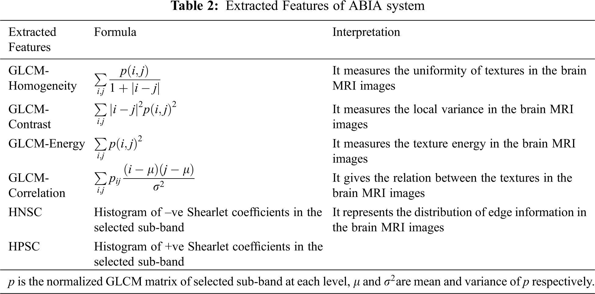
The selected directional sub-bands are utilized for extracting features such as GLCM [25], HPSC, and HNSC. GLCM features are extracted with one pixel difference and at four angular directions; 0, 45, 90 and 135 degrees. Also, HPSC and HNSC features use 10 bin histograms to reduce the feature space. Tab. 2 shows the features used by ABIA system for brain MRI image classification. The number of features extracted at any angular direction of GLCM is 4 and thus 16 GLCM features are extracted from four angular directions. Also, a total of 20 histogram features are obtained from HPSC and HNSC. Thus, the ABIA system uses 36 features for the classification.

2.2 Classification of MRI Brain Images

The selection of good classification algorithm is also an important step to achieve higher accuracy. In the ABIA system, a hybrid classification is employed with three different classifiers; kNN, NB and SVM classifiers. The output of individual classifiers for a testing input is hybridized to take a final decision for the classification of brain cancer. Fig. 4 shows the hybrid classification stage of the brain image classification system.

Figure 4: Hybrid classification stage of ABIA system

2.2.1 kNN Classifier

kNN [12] is performed by finding the k nearest neighbours in the feature space defined by the feature vector. The feature vector of ABIA system is the combination of features (GLCM + HPSC + HNSC) extracted from the selected NSST sub-bands at each level. Each neighbour votes on the classification of the testing sample. The closeness of neighbours in n-space is calculated from the n-dimensional Euclidean distance metric. Let us consider two feature vectors with n-dimension; f1=(x1,x2,x3,…xn) and f2=(y1,y2,y3,…yn) . The Euclidean distance between them is defined by

Euclidean distance

(f1,f2)=(x1−y1)2+(x2−y2)2+…+(xn−yn)2 (9)

There is no training phase in kNN. Hence, it is classified as a lazy classifier. As the computation of Euclidean distance requires all of the training objects each time, kNN requires more storage space and more calculation at the time of classification.

2.2.2 NB Classifier

NB classifier [13] uses Bayesian inference for the classification with an assumption that features of different classes are independent of one another. This assumption reduces the computational complexity as small amount of training data is required to train the classifier in 1-dimensional space n times where n is the number of features. If the features are assumed to be related to one another, then the testing object needs to be classified in n-dimensional space.

The posterior probability defined by Bayes theory is the probability that the object belongs to kth class based on its feature vector. It is defined by [13]

P(Ck|f1,.......fn)=1Zp(C)∏i=1np(fi|Ck) (10)

where, Z=∑kp(Ck)p(f|Ck) is a scaling factor depends on the feature vector. Since, NB classifier needs only the trained model for testing; it has a fast operational phase.

2.2.3 SVM Classifier

In many machine learning applications, SVM classifier [26] is used as a classification tool. It is very useful for two-class and multi-class classification problems. Let T {(fk,ck),k=1,2,3,...N} be the training data and u be the unknown data. A linear discriminant function with T and u is defined by Cortes et al. [26]

O(u)=wTu+b (11)

where the bias(b) and weight(w) are computed using T. The hyperplane defined in (12) separates the features in T optimally [26].

minw,b12‖w‖2+C∑j=1kξjsubjecttocjO(tj)≥1−ξj,andξj≥0,k=1,2,....n. (12)

where the trade-off parameter (C) controls the trade-off between complexity and empirical risk.

O(u)=∑j=1MscjαjK(u,vj)+b (13)

where the support vectors are vj,j=1,2,.....Ns computed from structural risk minimization and K(∙) is the kernel function. As SVM-RBF kernel produces more accuracy in Ayalapogu et al. [11], the ABIA system also uses RBF kernel. It is defined by [26]

K(u,v)=exp⁡(‖u−v‖22σ2) (14)

where σ is the standard deviation.

2.2.4 Hybrid Approach

The final decision of ABIA system is made from the classification results of each classifier to obtain a better decision. It combines the robustness of each classification algorithm and eliminates their drawbacks. Let di be the decision from ith classifier and wi be the weight of ith classifier. The final decision fd is defined by

fd=∑i=1kdiwi (15)

where k is the number of classifiers used. The weight of each classifier is assigned to their accuracy when using different training samples.

3  Results and Discussions

The performance of ABIA system to classify brain MRI images is evaluated by using the standard set of brain tumor images available in the REMBRANDT database [27–29]. It consists of MRI brain images collected from 130 subjects. All images are in DICOM format with resolution of 256 × 256 pixels. From the vast number of images, 100 images in each category (normal/abnormal) are selected [11]. Fig. 5 shows REMBRANDT database brain MRI images.

Figure 5: REMBRANDT database -brain MRI images (a) Normal (b) Low grade (c) High grade

The ability of ABIA system to classify all brain MRI images is measured by classification accuracy ( Acc ). Also, the ability to classify abnormal and normal brain MRI images is measured by sensitivity ( Sen ) and specificity ( Spe ) respectively. Tab. 3 shows the evaluation index of ABIA system.

Tab. 4 shows the Acc of NA stage for different NSST levels and directions at each level. It is also stated that NSST is a multi-scale analysis in frequency domain, the performance of ABIA system is evaluated for the features from different NSST levels (from 1 to 4) and at different directions (powers of 2 up to 5).

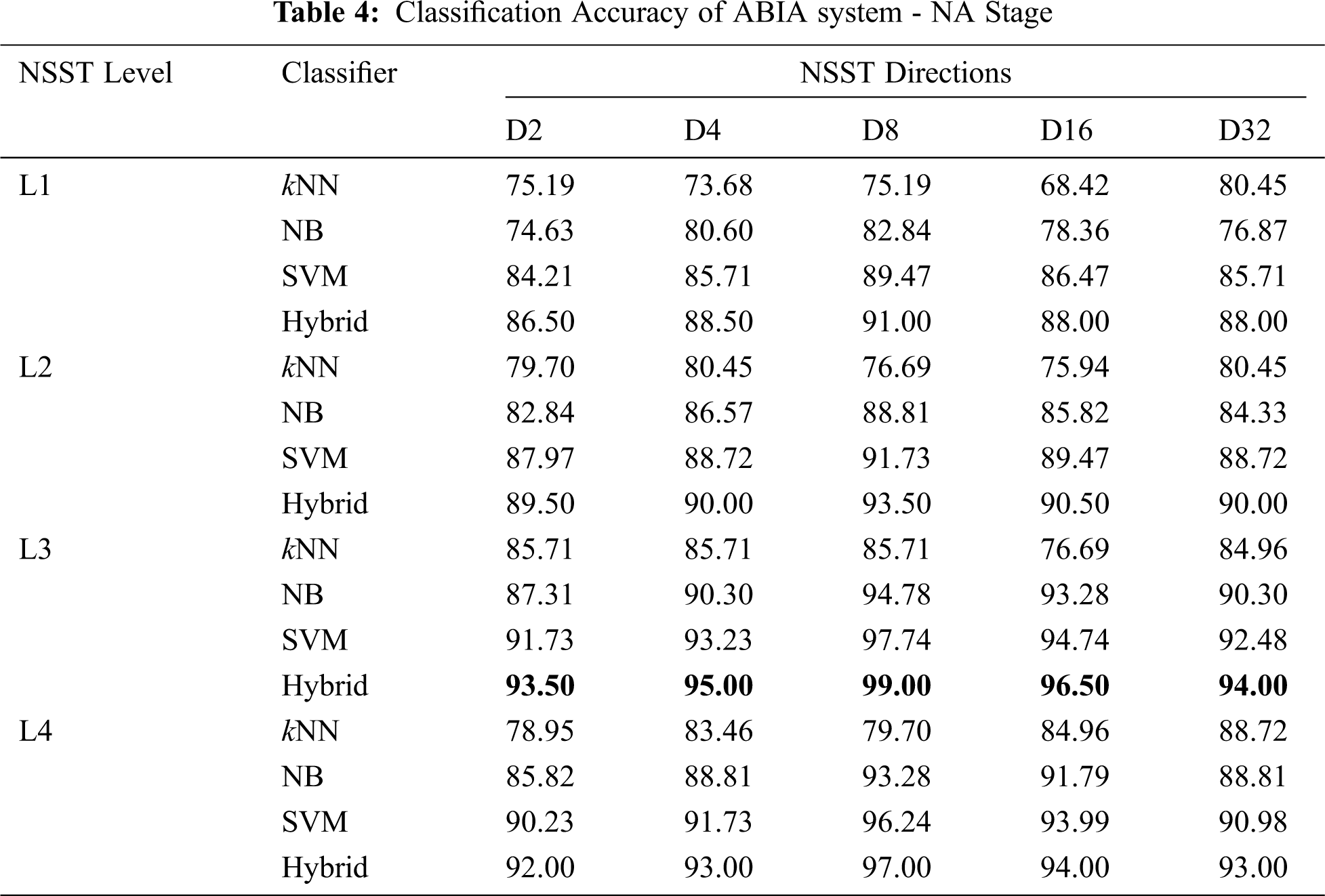
It is observed that the hybrid approach gives much higher performance in L3-D8 than other combinations. Also the Acc of individual classifier is in the order of SVM > NB > kNN. In particular, the maximum Acc of hybrid classification is 99% while the maximum Acc of 85.71%, 94.78% and 97.74% is observed when using kNN, NB and SVM classifier respectively. As NSST produces more redundant information at higher levels with higher directions, the performances of ABIA system is decreased. It can be seen from the obtained Acc from L3 to L4 and D8 to D16 and D32 at each level. Tab. 5 shows the Acc of LH stage for different NSST levels and directions at each level.

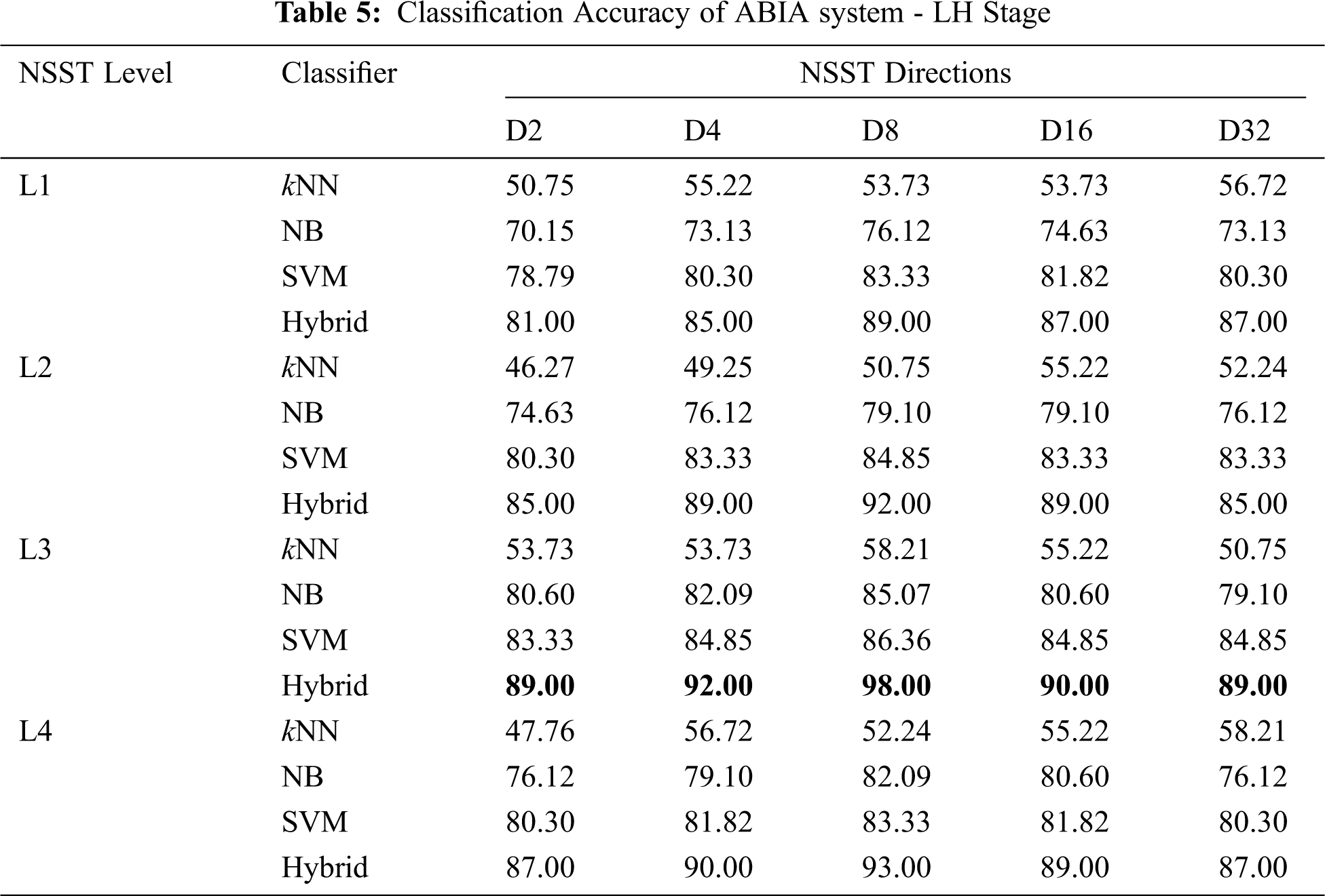
It is observed from Tab. 5 that the LH stage of ABIA system also produces higher performance in L3-D8 than others. The hybrid approach yields an Acc of 98%. Among the individual classifiers, SVM and NB achieve more than 80% Acc whereas the Acc of lazy classifier is below 60%. The obtained results in Tabs. 4 and 5 show the significance of NSST as a feature extraction approach for the ABIA system. Fig. 6 shows the Receiver Operating Characteristics (ROC) for the best performance (L3-D8 features) of ABIA system.

Figure 6: ROCs of ABIA system- LH stage (left image) and LH stage (Right image)

Figs. 7 and 8 show the other performances such as Sen and Spe for NA stage and LH stage respectively using the combination of features from L3-D8.

Figure 7: Performance comparison of individual classifier with hybrid approach – NA stage of ABIA system

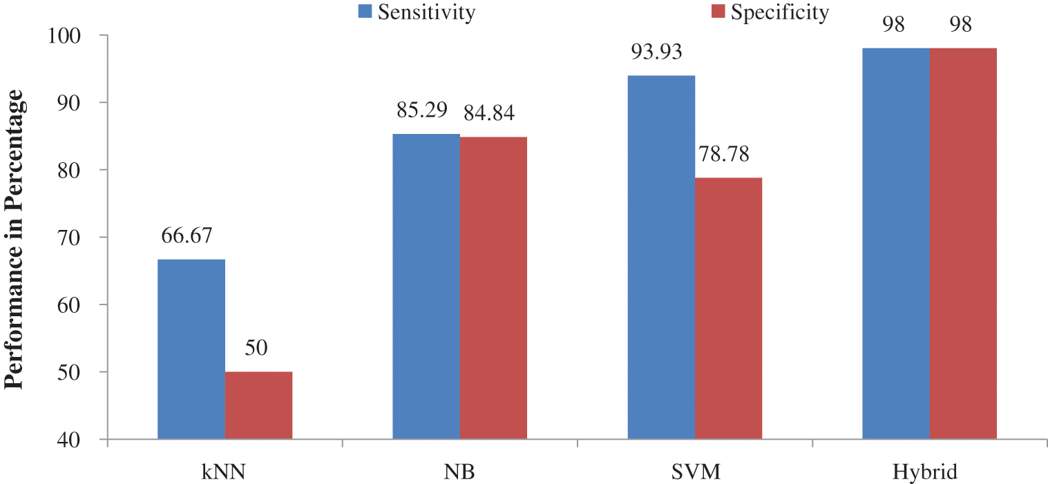
Figure 8: Performance comparison of individual classifier with hybrid approach – LH stage of ABIA system

It is observed from the performance comparisons in Figs. 7 and 8 that hybrid approach performs well than their individual counterpart. It is obvious that kNN is the least performer as it is a lazy classifier. Tab. 6 shows the comparative study of ABIA system with existing approaches using REMBRANDT database images. Also they are designed to classify them into normal or abnormal category only. Thus, the performance of existing approach is compared with the performance of NA stage of ABIA system.

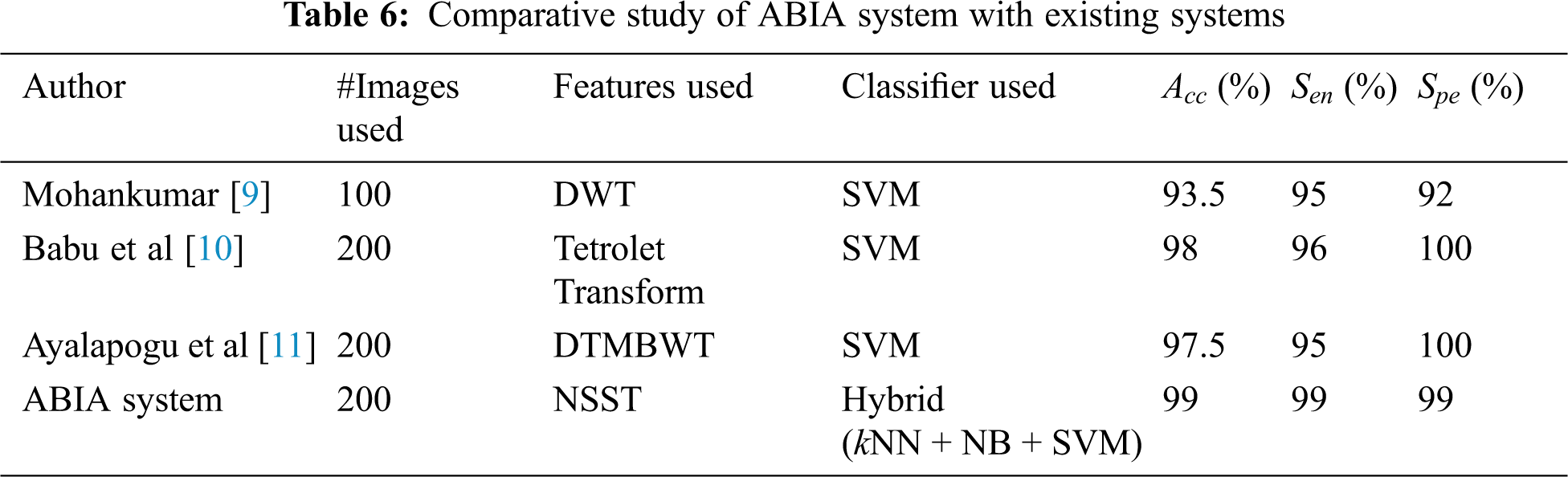
From Tab. 6, it is observed that the ABIA system is able to achieve near perfect sensitivity and specificity. Also, the performance of ABIA system shows a statistically significant difference in the accuracy of existing systems. From the performances of ABIA system, it is concluded that the ABIA system could potentially decrease the physician bias seen in ROI analysis. The output of ABIA system gives an alarm to the radiologist who can still examine the image for further review.

4  Conclusions

In this paper, an ABIA system to classify brain MRI images is discussed. The most correlated NSST sub-band at each NSST level is selected by t-test on training data set. The ABIA system uses the combination of features that includes GLCM, HPSC, and HNSC as indicators for the characterization of brain MRI images. Then, the extracted features are trained by a hybrid classification approach that includes kNN, NB and SVM. A two two-class classification system (NA stage and LH stage) is designed to classify brain MRI images. Results show that the clinical applicability of ABIA system for brain MRI image classification with an accuracy of 99% for NA stage and 98% for LH stage using the hybrid approach.

Funding Statement: The authors received no specific funding for this study.

Conflicts of Interest: The authors declare that they have no conflicts of interest to report regarding the present study.

This work is licensed under a Creative Commons Attribution 4.0 International License, which permits unrestricted use, distribution, and reproduction in any medium, provided the original work is properly cited.