DOI:10.32604/csse.2022.017931
| Computer Systems Science & Engineering DOI:10.32604/csse.2022.017931 | |
| Article |
Dates Fruit Recognition: From Classical Fusion to Deep Learning
1Department of Computer Science, College of Computer, Qassim University, Buraydah, Saudi Arabia
2Department of Information Technology, College of Computer, Qassim University, Buraydah, Saudi Arabia
3Department of Computing, School of Electrical Engineering and Computer Science (SEECS), National University of Sciences and Technology (NUST), Islamabad, Pakistan
*Corresponding Author: Ali Mustafa Qamar. Email: al.khan@qu.edu.sa
Received: 17 February 2021; Accepted: 18 April 2021
Abstract: There are over 200 different varieties of dates fruit in the world. Interestingly, every single type has some very specific features that differ from the others. In recent years, sorting, separating, and arranging in automated industries, in fruits businesses, and more specifically in dates businesses have inspired many research dimensions. In this regard, this paper focuses on the detection and recognition of dates using computer vision and machine learning. Our experimental setup is based on the classical machine learning approach and the deep learning approach for nine classes of dates fruit. Classical machine learning includes the Bayesian network, Support Vector Machine, Random Forest, and Multi-Layer Perceptron (MLP), while the Convolutional Neural Network is used for the deep learning set. The feature set includes Color Layout features, Fuzzy Color and Texture Histogram, Gabor filtering, and the Pyramid Histogram of the Oriented Gradients. The fusion of various features is also extensively explored in this paper. The MLP achieves the highest detection performance with an F-measure of 0.938. Moreover, deep learning shows better accuracy than the classical machine learning algorithms. In fact, deep learning got 2% more accurate results as compared to the MLP and the Random forest. We also show that classical machine learning could give increased classification performance which could get close to that provided by deep learning through the use of optimized tuning and a good feature set.
Dates are usually a brown, oblong-shaped fruit that grows on palm trees. They are mostly eaten in a dried state. This fruit is cultivated worldwide in countries like Egypt, Iran, Iraq, Pakistan, Saudi Arabia, and the UAE. Presently, India, Morocco, UAE, Indonesia, and Turkey are the biggest importers of dates globally. On the other hand, the consumption of dates fruit is increasing at a steady rate, and Africa has become its largest consumer. Similarly, North America is the fastest-growing market for dates. Although dates are cultivated in many countries, the Middle Eastern ones are the most sought-after owing to their excellent taste.
The date fruit is a rich source of Calcium, Potassium, Vitamin C, and Iron. Furthermore, dates have certain features that help in recognizing and classifying them into different classes. The main features include color, texture, and shape. This paper thus performs image-based dates fruit classification and recognition by creating a nine-class dataset. The classes are Sukkari, Ajwa, Barhy, Hasheshy, Khalas, Majdool, Munefee, Rothanah, and Sugee. As far as we are aware, there exists no previous work where researchers have used the aforementioned classes for dates’ recognition while conducting extensive experiments with various machine learning and deep learning algorithms. This dataset also presents a competitive framework for computer vision algorithms. This research uses various feature extraction approaches and then merges these approaches. Here, four classical machine learning algorithms are used for classification. Moreover, deep learning is also explored for dates’ recognition.
Pourdarbani et al. [1] presented an online sorting system to sort dates at various stages of maturity, namely Khalal (changing color, though not mature), Rotab (mature), and Tamar (ripe), as shown in Fig. 1. Offline tests were carried out on 50 samples for each stage to extract color and texture features. The color features were significantly different for the three stages. Furthermore, 100 samples were used during the online experiments. They got an average detection rate of 88.33%. Human experts could also detect only 91.08% of the dates. The least detection rate was reported for Rotabs on the verge of Tamar since it looked similar to the latter.
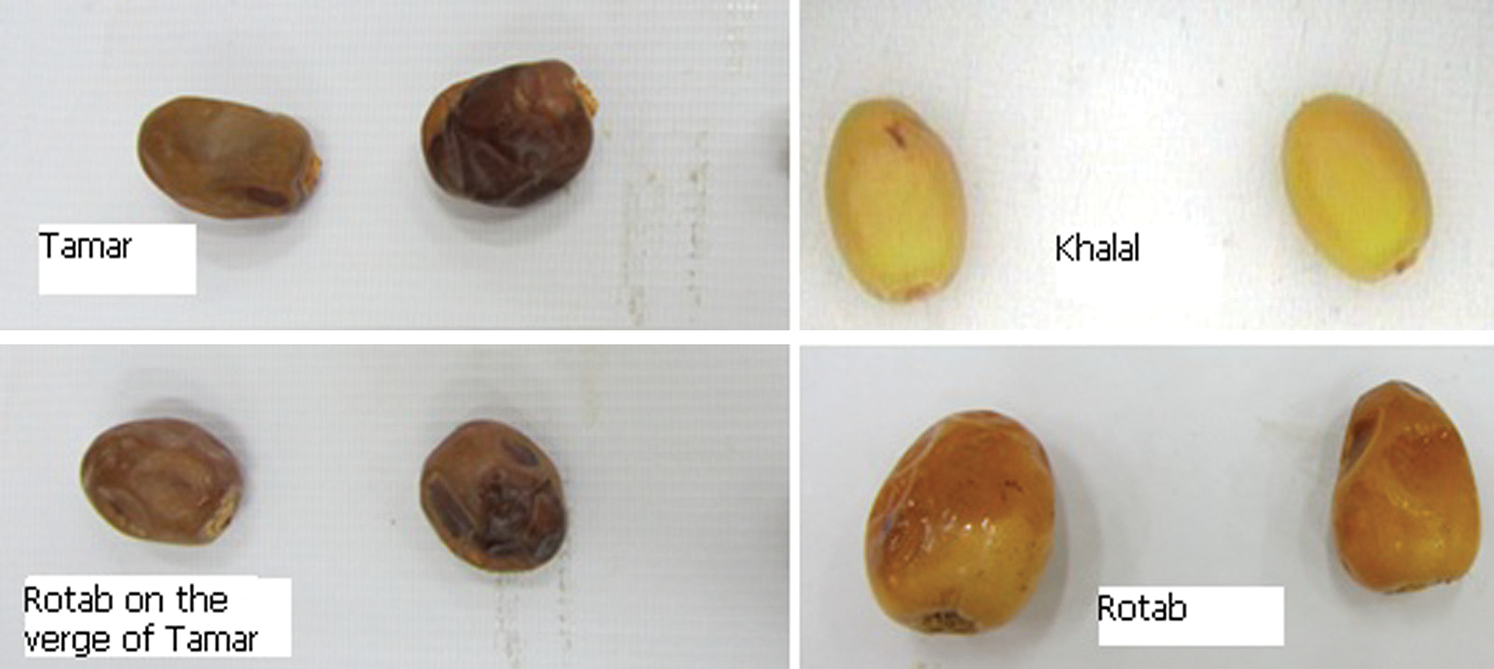
Figure 1: Dates at various stages of maturity [1]
Dates’ growers usually harvest in a period of three to four weeks, thus getting dates with different maturity stages [2]. The unripe dates are either placed in a hydrating building to gain moisture (most mature), left in the sunlight (medium), or put in a heated building to dry (least mature). Whereas inadequate drying can make the dates sour, excessive drying can cause its skin to peel, resulting in lower quality. Lee et al. [3] worked on 700 Medjool dates and achieved an average accuracy of 90.86%. They came up with a practical color mapping concept for automatic color grading. The proposed method maps the RGB values of colors of interest to color indices. The various maturity levels with dates range from yellow to dark red, with orange and light red in between, as shown in Fig. 2. Their results were consistent with human grading. They achieved an accuracy of 87% on a data set of 2118 dates.
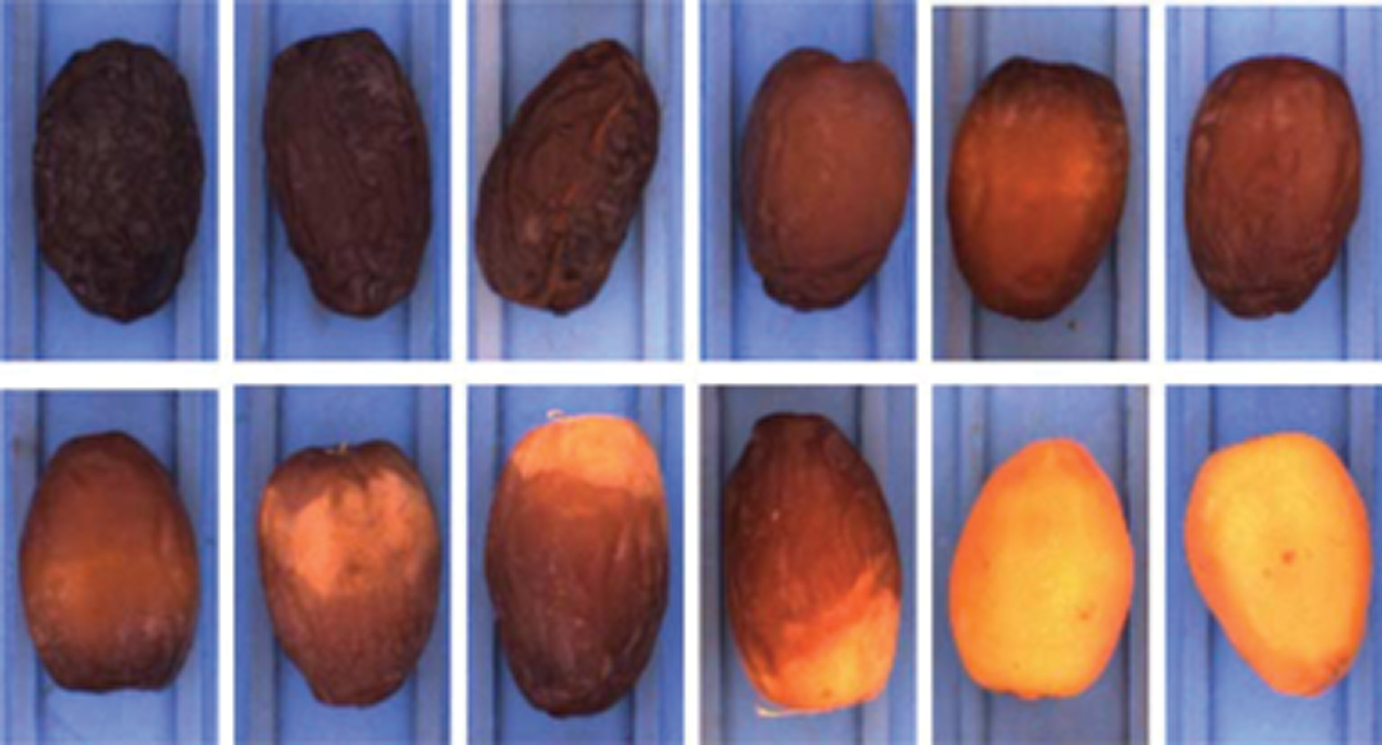
Figure 2: Various maturity stages for dates [3]
Pandey et al. [4] reviewed automated fruit grading systems. The algorithms are primarily based on either machine learning or color. Ohali [5] classified dates based on size, shape, and intensity. They got an accuracy of 80% while using a backpropagation neural network. Haidar et al. [6] classified dates using linear discriminant analysis. They used seven types of dates, such as Sukkari, Mabroom, Khedri, Safawi Al Madina, Madina Ajwa, Amber Al Madina, and Safree. The dataset comprises 140 images in JPEG format, having a size of 480 × 640 pixels. Their approach got 99% accurate results while employing Artificial Neural Networks (ANN). Alresheedi [7] used nine classes of dates with four classifiers. The four classifiers include Random forest, Bayesian network, Multi-layer Perceptron (MLP), and the Support Vector Machine (SVM). Gabor features and Color Layout features are used as dates’ features. These features are then fused to increase classification performance. The proposed approach achieve an acceptable performance of over 88% correct detections.
Zawbaa et al. [8] used a random forest to classify fruits such as strawberries, oranges, and apples. They used features such as shape, color, and the Scale Invariant Feature Transform. The results obtained with random forest were better than those using k-nearest neighbors and SVM.
Arivazhagan et al. [9] discuss an efficient combination of color and textual features for fruit discrimination. The recognition was made by the minimum distance classifier using statistical and appearance features derived from the Wavelet convert sub-bands. The testing results on a database of about 2635 fruits from 15 classes show their suggested method’s performance. In another paper [10], the authors explore how to merge the input from various bottom-up segmentation of the images to perform object recognition validity by combining the image segmentation supposition in a conjectural collective top-down and bottom-up recognition path. They also enhance the object and feature boost. Aldoma et al. [11] suggest two-dimensional and three-dimensional computations of RGB-D data to perform object recognition without loaded tissue and globally repeated characterization of the object models’ prototypal adjective. Satpathy et al. [12] discuss two groups of novel edge-texture features, Discriminative Robust Local Binary Pattern (DRLBP) and Ternary Pattern (DRLTP) for object admission. By examining the restriction of Local Binary Pattern (LBP), Local Ternary Pattern (LTP) and Robust LBP (RLBP), DRLBP and DRLTP are suggested as new features. They resolve the issue of recognition between a vivid object against a dark background and vice versa.
Zhao et al. [13] proposed four types of deep learning based on fine-grained image classification, including the general convolutional neural networks (CNNs), portion exposure, a crew of networks base, and visible concern based on fine-grained image classification methods. In the paper [14], the authors discuss the leading deep learning concepts relevant to medical image analysis and cover over 300 contributions to the domain. They studied deep learning for image classification, object detection, segmentation, and registration. They provided short sketches of studies per application field. In another article [15], the authors show a judicial spatial refreshed deep belief network that appropriates locative data Hyper Spectral Image (HSI) classification. HSI is head segmented within the adaptive line arrangement based on spatially alike sections with similar spectral characteristics in the suggested method. In the paper [16], the authors review the classification of wood boards’ quality based on their images. It compares deep learning, especially CNN, combined with texture-based feature extraction systems and popular methods: Decision tree induction algorithms, Neural Networks, nearest neighbors, and SVM. Their results show that Deep Learning techniques applied to image processing tasks have better predictive performance than popular classification techniques, specifically in highly complex situations.
This section introduces the main methodology of the proposed work. The approach starts with feature extraction, which is followed by feature selection. After feature selection, the machine learning algorithms are used to learn the dates’ classes.
The generic approach for dates’ classification is like every other computer vision approach. The images of the dates are selected for analysis. The features are then extracted using the feature extraction approach. The feature extraction approach dominates the classification performance of the dates. Therefore, this stage is crucial to the overall detection performance. In this work, four feature extraction approaches are used, namely Color Layout Features, Fuzzy Color and Texture Histogram (FCTH), Gabor approach, and the Pyramid Histogram of the Oriented Gradients (PHOG). These approaches are explained in the following subsections. The machine learning set includes the Bayesian network, SVM, Random Forest, and MLP. Feature fusion is used to increase the classification performance.
Fig. 3 shows the flow of the steps for deep learning. The steps are explained as follows:
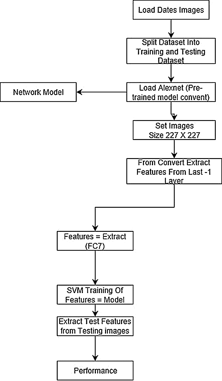
Figure 3: Algorithmic steps for the deep learning algorithm
Before applying CNN, the dataset must be loaded into memory. Furthermore, the deep learning experiments assume the data has been divided into two sets: the test set and the training set. The deep learning experiments have two dimensions in training: the first is to train the network on the dataset of concern, while the other is to use already trained models. The first one is time-consuming and usually has weaker performance compared to the second one. The latter, which uses the already-trained model, is called transfer learning and is becoming a standard in deep learning research. In the present paper, we opted for the transfer learning approach.
The transfer learning approach helps in learning the good features from images and saves execution time and resource allocation. In fact, we use ALEXNET (ANET), sometimes also called CONVNET. This network has already been trained for 1000 categories on 1.3 million images, and has robust performance. It is worth noting that once loaded in memory, this network has several layers.
We then need to set our images’ size according to the ALEXNET’s standard size, which is 227 × 227. With this setup, we are ready to extract the deep features from the deep learning network. In order to do so, we use the FC7, which is the last layer before classification (SVM). We use this layer for image feature extraction because it is suggested by the general image and computer vision framework and the state-of-the-art, especially for images.
Once the features are extracted from the FC7, they are then learned using the SVM classifier. Other classifiers can be integrated into this layer. After performing feature extraction from the training data, the test data has also to pass through these stages for feature extraction. The classifier, which has now learned the model from the training images, uses the training model to classify the test images. After this comparison, the deep network reports the performance.
For classical features analysis, four feature extraction approaches are used. These are Color Layout Features, FCTH, Gabor approach, and PHOG.
The color layout features are defined as follows:
• Dominant color comprises the dominant colors, the percentage, the variance, and the spatial based coherency
• Color structure - the global and local spatial color structures in an image
• Scalable color - or a HAAR transformation applied to the values of a color histogram
• Homogeneous Texture - Quantitative texture
• Edge Histogram - the spatial distribution of edges which represent local distribution in the image
• Contour-based shape - the contours of the objects
These features are extracted in WEKA [17] using the Color Layout Filter. This filter divides an image into 64 blocks and computes the average color for each block, and then the features are calculated from the averages.
3.2.2 Fuzzy Color and Texture histogram (FCTH)
Fuzzy Color and Texture histogram (FCTH) are presented in Chatzichristofis et al. [18]. As the name suggests, these features encode both color and texture information in one histogram. According to [18], a Conventional Color Histogram does not consider the color similarity across different bins. It also does not consider the color dissimilarity in the same bin. It is very sensitive to noise in images, for example, the illumination changes and the quantization errors. Furthermore, they are considerably large, which is not feasible for large datasets. The FCTH considers the similarity of each pixel’s colors regarding all the histogram bins using the fuzzy-set membership function. This approach shows superiority over the traditional color histograms.
The Gabor filters, especially the 2D versions, find many applications in image processing. They are instrumental in feature extraction for texture analysis and segmentation. Gabor filter contains a set of filters having different frequencies and orientations. The filter set is helpful in computer vision and is used primarily for feature extraction from an image. The 2D Gabor filters are represented by Eqs. (1) and (2):
In Eqs. (1) and (2), the symbols B and C are termed normalizing values and are determined during processing; f is the frequency searched in the texture. By changing the θ, we look for texture orientation in a specific direction. The σ represents the image region’s size being analyzed, Gc represents the real part, and Gs depicts the imaginary part. In our experiments B is taken as 100, and C is fixed at 10.
3.2.4 Pyramid Histogram of Oriented Gradients (PHOG)
PHOG [19] are descriptors based on the spatial arrangement of pixels and objects in an image. They describe an image in its spatial layout and local shape features. The PHOG descriptors are composed of the Histogram of Gradients (HOGs) over each image sub-region. The image is divided into sub-regions represented at the pyramid resolution level. The local shapes in an image are captured by the distribution over edge orientations within a region, while the spatial layout is captured by tiling an image into regions at multiple resolutions.
Classifiers learn the separating plane in the dataset characterized by class differentiation. We discuss the following classifiers, which are used in experimentation and analysis.
Bayesian Networks (BN) represents the variables and their relationship using a Direct Acyclic Graph (DAG). BN is based on statistical theories and uses probability distribution, and hence is known as a parametric classifier. DAG represents the relation between a set of random variables and their dependence on each other. In Hedman et al. [20], BN has been used for the analysis of environmental changes. The experiment was carried out using Synthetic Aperture Radar data. Because of BN networks’ widespread use, several enhanced BN versions have been proposed, such as BART [21]. However, BART is limited to classifying only two-class problems and hence cannot be used for multi-class problems. To cope with these problems, another enhanced version of BN called mBACT has been proposed. In Agarwal et al. [22], the performance of mBACT has been investigated in the classification of low-resolution Landsat imagery. The results showed that mBACT performed better than SVM and Classification and Regression Tree.
3.3.2 Support Vector Machines (SVM)
The SVMs are also called Support Vector Networks [23]. The learned model assigns newly sampled data to one of the categories, making it a non-probabilistic binary linear classifier model. In SVM, the data can be visualized as points in space which are then mapped to another space so that the hyperplane separates the data. The new test data is then mapped to the same space and predicted to belong to a category depending on the hyperplane. SVM can also be used for non-linear classification by using a kernel. Kernel maps are high-dimensional feature spaces where separation becomes easy.
Lately, tree-based classifiers have gained substantial admiration. The Random Forest was developed by Breimen [24], where Random receipts benefit from the mixture of several trees from the identical dataset. The random forest creates a forest of trees, and each tree produced is based on the random kernel. For classification stages, the input vector applies to every tree in the forest. Each tree decides the class of the vector. These decisions are then summed up for the final classification. The tree’s decision is termed as the vote of the tree in the forest, and the random forest works on majority voting.
For growing the classification trees in the random forest, let there be N cases in the training set. Thus, sampling N data items are selected randomly but picked based on a replacement from the data set. This sample makes up the training set for tree growth. If there are K variables, a small k, where k << K is specified, such that at each node, k variables are selected randomly from the large K. The best split on this k is used to split the node, and the value of k is held constant during the forest growth. Each tree can grow to its largest possible extent on its part of data since there is no pruning. With the increase in the tree count, the generalization error converges to a limit.
3.3.4 Multi-Layer Perceptron (MLP)
A Multilayer perceptron is a type of neural network, feed-forward ANN, that works by plotting the data variable from a dataset over output descriptions. Commonly, this is significantly more heterogeneous than the perceptron. It consists of two or more layers of artificial neurons by combining non-linear activation roles. The non-linearity and the non-linear activation functions are in fact, developed to model the action potential frequency or firing of human neurons in the brain [25]. As in the general neural network model, each node in one layer connects in a certain way to every other node in the following layers. The learning framework is based on the backpropagation algorithm [26], which corresponds to changing the way after every training cycle. This modification of the way is carried out according to the error between inputs and the label prediction.
We present the detailed analytical results for the nine classes of dates for four classifiers: Bayesian network, SVM, Random Forest, and MLP. These classifiers are selected according to their excellent performance in the state-of-the-art. The four parameters of performance used in this paper are accuracy, precision, recall, and F-measure.
4.1 Fuzzy Color and Texture Histogram (FCTH)
Fig. 4 shows the result of four parameters with the four classifiers using FCTH.
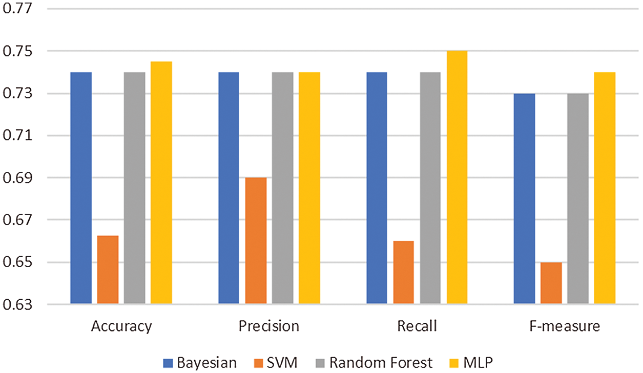
Figure 4: Fuzzy Color and Texture Histogram (FCTH) performance
The MLP achieves slightly higher accuracy (0.745) than Bayesian and Random forest. The SVM reports a decreased classification performance of only 0.66. Precision almost follows the trend of accuracy where the MLP, Bayesian, and Random Forest achieve the highest precision of 0.74 while SVM reports a decreased precision of 0.69.
The recall also almost follows the trend of accuracy. The MLP achieves the highest recall of 0.75. The SVM reports a decreased classification performance of 0.66. The Bayesian and Random Forest report a recall of 0.74, which is slightly lower than the MLP and higher than that obtained while employing SVM. The MLP achieves the highest F-measure of 0.74. The SVM reports a decreased classification performance with an F-measure of 0.65. The Bayesian and Random Forest report an F-measure of 0.73.
4.2 Pyramid Histogram of Oriented Gradients (PHOG)
Fig. 5 shows the result while using PHOG.
The Bayesian network achieves the highest accuracy of 0.863. SVM and MLP report a decreased classification performance of 0.81. The Random forest reports an accuracy of 0.833. The Bayesian network achieves the highest precision of 0.86. The SVM and MLP report a decreased precision of 0.81. On the other hand, Random Forest reports a precision of 0.84. The Bayesian network achieves the highest recall of 0.86. The SVM and MLP report a decreased recall of 0.81. Random Forest reports a recall of 0.83. The Bayesian network achieves the highest F-measure of 0.86. The SVM and MLP report decreased F-measure of 0.81. The Random Forest reports an F-measure of 0.83.
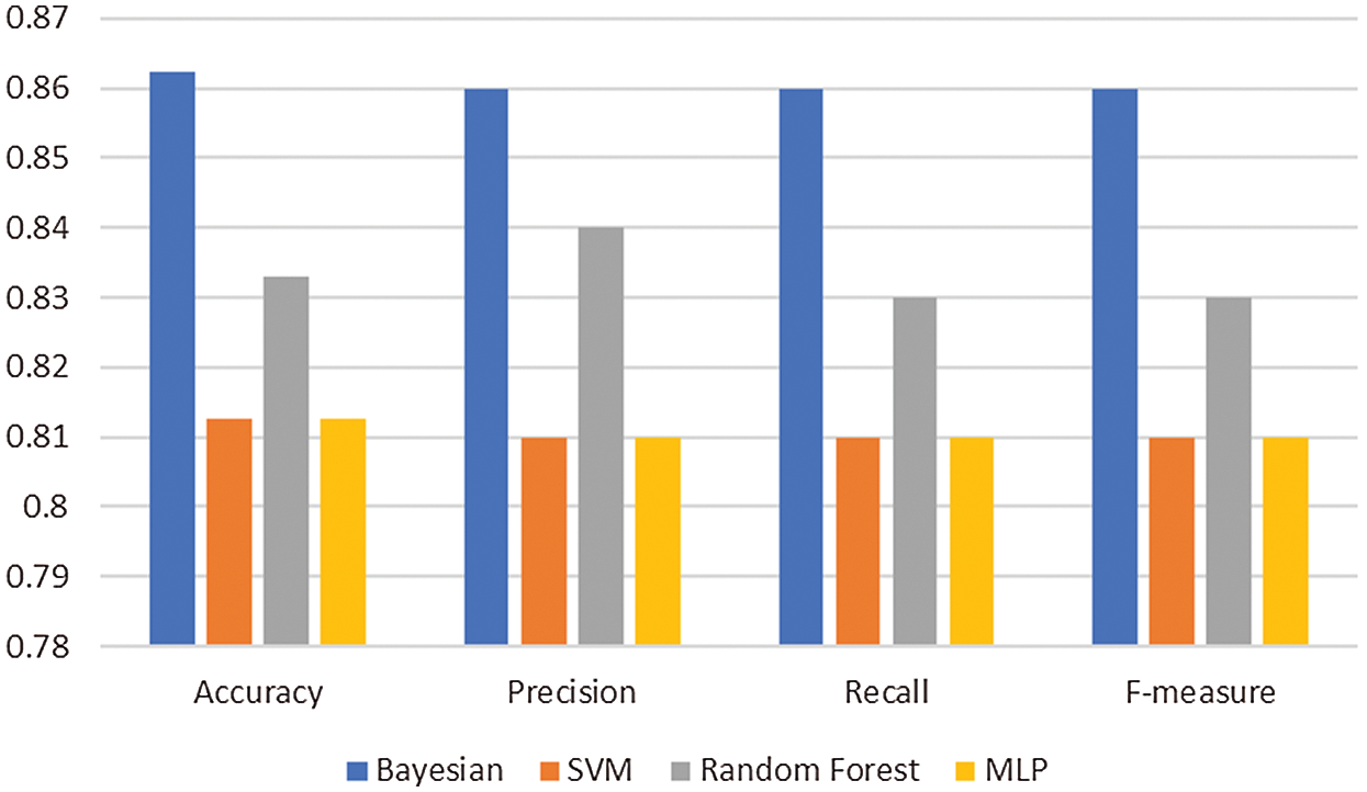
Figure 5: PHOG filter performance for nine classes
For performance enhancement, we propose feature fusion. The feature fusion is realized as follows:
Fig. 6 shows the performance analysis of the fusion approach of PHOG with the Gabor filter. The fusion approach outperforms the Gabor approach in all the cases with a high margin.
In the Bayesian network case, the fusion approach has an increased F-measure of 2% compared with the PHOG and more than 40% compared with the Gabor. For SVM, the fusion approach has an increased F-measure of 6% compared to the PHOG and 37% compared to the Gabor. In the Random forest case, the fusion approach has an increased F-measure of 6.6% compared to the PHOG and 38% compared to the Gabor. In the case of the MLP, the fusion approach has an increased F-measure of 6.5% compared to the PHOG and 36.5% compared to the Gabor approach.
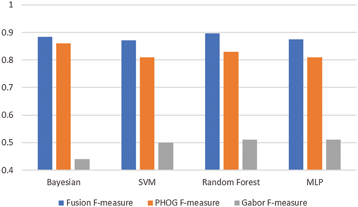
Figure 6: Fusion of the two features (PHOG and the Gabor filters) gives increased classification performance in all the cases compared to the unfused single features
Fig. 7 shows the performance analysis of the fusion approach of PHOG with the FCTH. The fusion approach outperforms the FCTH approach in all the cases with a high margin.
In the Bayesian network case, the fusion approach gets an F-measure, which is more than 5% better than PHOG and 18.2% better than FCTH. For SVM, the fusion approach has an increased F-measure of 11.1% compared to PHOG and 27.1% compared to FCTH. In Random forest, the fusion approach has an increased F-measure of 9.5% compared to PHOG and 19.5% compared to FCTH. With MLP, the fusion approach has an increased F-measure of 12.8% compared to PHOG and 19.8% compared to the FCTH.
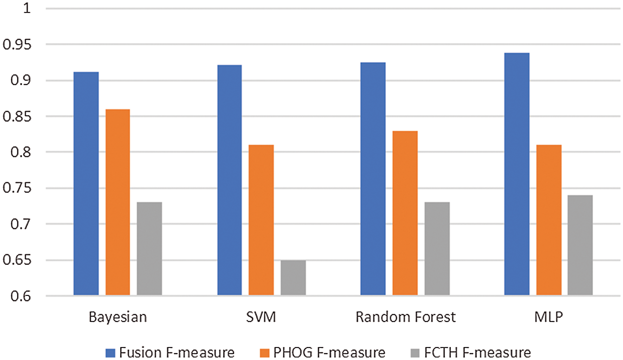
Figure 7: Fusion of the two features (PHOG and the FCTH) gives increased classification performance in all the cases compared to the unfused single features
Fig. 8 shows a comparison of the three fusion approaches based on F-measure. These three fusion approaches are PHOG + FCTH, Gabor + PHOG, and the Color layout + Gabor.
We use the results reported by Alresheedi [7] for the fusion of color layout + Gabor. The fusion of PHOG and the FCTH shows an increased classification performance for all four classifiers, the highest F-measure being in the case of the MLP. The HOG-based feature set combined with the fuzzy color histogram optimally models the dates and achieves an F-measure of almost 0.91. The fusion of Gabor + PHOG also has good classification performance with Bayesian, Random forest, and the MLP. In SVM, it has slightly decreased classification performance compared to the color + Gabor. The Color layout + Gabor shows a decreased classification performance in all cases except for SVM, where it slightly outperforms the Gabor + PHOG.

Figure 8: F-measure of three fusion approaches
Here, we use shape features only and compare the performance of classification. The shape features are Area, Eccentricity, Major Axis, and Minor Axis. We select these features as they are already used in the state-of-the-art and provide a base for comparison. Fig. 9 shows the performance analysis of the shape features.

Figure 9: Shape-based analysis of dates
The MLP leads the performance in every case. Bayesian has the lowest performance in all cases. SVM has a lower performance than Random forest in three cases and a similar performance in the case of precision. The Random forest has higher accuracy, recall, and F-measure as compared to MLP and SVM. We got the least F-measure with this analysis, the highest being just 0.604. This is not a good result, and the model cannot be used for practical purposes. Therefore, we believe that shape on its own cannot be considered a useful feature for dates analysis. The main reason is that dates can continuously change over time, either naturally or due to pressing in both handling or packaging. Therefore, if color and texture features are not added to the shape, the dates model is not accurate.
Fig. 10 shows a comparative analysis of the fusion approach with the state-of-the-art approach by Muhammed [27], which uses the texture + shape features. For this comparative analysis, we implemented the approach of Muhammed. The same dataset was used with both approaches. We extracted features using their approach and used them in WEKA.
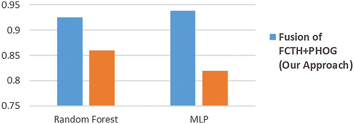
Figure 10: Comparative analysis of Random Forest and MLP
For this comparative analysis, we selected the Random Forest and MLP. We selected these two only because they have good overall performance in all the experiments. Our Fusion approach achieves an F-measure of 0.925 in the Random forest case, while the texture + shape features approach of [27] achieves an F-measure of 0.86. The Fusion approach achieves an F-measure of 0.938 in the case of the MLP, while the texture + shape approach achieves an F-measure of 0.82. This comparative analysis shows that the fusion of features can outperform shape and text features, especially for dates classification.
This paper’s primary focus is the analysis of nine classes of dates fruit in the light of different classifiers and features set. Therefore, most experimental results are reported on the performance calculation of the average value of F-measure, accuracy, precision, and recall. However, in this subsection, we focus on one set of experiments to show each of the dates fruit’s specifics. The experiment we select is that of the Random forest with the fusion features of PHOG + FCTH. We select this experiment due to a higher value to F-measure as compared to others. Fig. 11 shows the F-measure for nine types of dates.
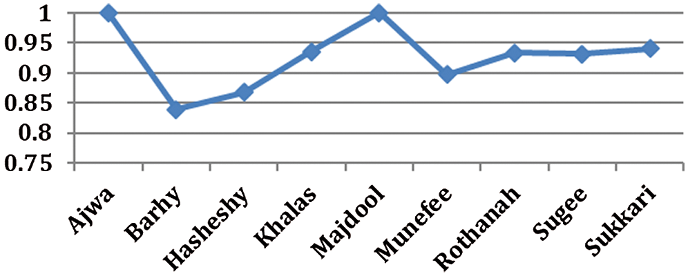
Figure 11: F-measure for the Random forest with PHOG+FCTH
One can observe individual dates and their corresponding performance values. As the F-measure summarizes precision and recall, we explain the analysis in terms of the F-measure. Also, the F-measure performance is directly related to a 100% sample comparison. Based on this, the following discussion summarizes the dates’ fruit analysis based on the particular dates.
Ajwa achieves an F-measure of 1. The Barhi date has an F-measure of 0.839. Barhi has low detection performance for two reasons: firstly, this class of date is quick to dry; secondly, it has color changes inside the class and has no formal shape. The Hasheshy date has an F-measure of 0.867, which is slightly higher than that of Barhi. Khalas date gets an F-measure of 0.935. This is higher than the values for Barhi as well as the values for Hasheshy. The possible reason is that Khalas is easily recognized by humans as well. Therefore, we believe that the classifier has learned dates in the same manner as human experts.
Moreover, Majdool gets 100% detection. The reason behind this result is that Majdool is very different compared to the other dates. The Muneffee gets an F-measure of 0.897. One of the possible reasons for this result is that it is small in size and has no formal shape. In the F-measure graph, the Rothanah gets an F-measure of 0.933, which is almost the same for Khalas. A possible reason for Rothanah’s low learning could be that the dates from this class vary in color. The Sugee gets an F-measure of 0.931. This means that the Sugee is identified in a much better manner than Barhi. Finally, the Sukarri gets an F-measure of 0.94, making it classified slightly better than the Barhi, Khalas, and the Sugee.
4.7 Deep Learning vs. Classical Algorithms
In many classification tasks and challenges, deep learning always outperforms classical machine learning. Consequently, numerous researchers have investigated the reasons behind this superiority in performance. Accordingly, answering why deep learning is seemingly better than classical classifiers represents another objective of our research, which also stems from our desire to investigate this phenomenon. It is worth mentioning that in this paper, by classical classifiers we mean the classifiers that are not based on the neural network deep framework.
The PHOG+FCTH fusion of features in Section 4.3.2 obtained a very high detection rate (F-measure) of almost 0.94. This is an excellent result, and a practical realization of the system for any serious automation of dates is very much possible.
4.7.2 Convolutional Framework and the Performance Analysis
Convolutional Neural Networks (CNN), one of the deep learning models, convolves learned features with input data and uses 2D convolutional layers. It can be used to perform classification, extract learned image features and train an image classifier. Here, we used the MATLAB implementation of CNN, called Convnet by Krizhevsky et al. [28]. This image classification network was composed of five convolutional layers, max-pooling layers, dropout layers, and three fully-connected layers.
We used the Rectified Linear Units (ReLU) for the non-linearity functions. The ReLUs were used because they helped in decreasing the training time. In addition, the ReLU is faster in execution than the Tanh function. Similarly, the data augmentation techniques of image translations, reflections, and patch extractions were also used. The dropout layers were used to solve the problem of overfitting. The model was trained using stochastic descent, and the final model was obtained by training on two GTX 580 GPUs for six consecutive days. Fig. 12 shows the performance of dates recognition for the nine classes and ten runs based on accuracy.
Fig. 13 shows the comparative analysis of deep learning with the classical machine learning setup using the PHOG+FCTH features. Classical machine learning includes the MLP and the Random forest.
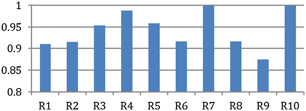
Figure 12: Accuracy of the ten runs of the CNN for dates
In Fig. 12, CNN with ALEXNET ran ten times, and the performance is reported. The network is executed ten times to measure the average of the ten runs. This mimics the ten folds cross-validation in the classical machine learning setup of the MLP and the Random forest. In run 7 (R7) and run 10 (R10), deep learning achieves almost 100% recognition rates. This is due to some of the dates’ classes. For example, if the training and testing sets include the Ajwa dates, the recognition capabilities increase due to the color of Ajwa, which is not present as such in other dates. Run 1 (R1), Run 2 (R2), Run 6 (R6), Run 8 (R8), and Run 9 (R9) show comparatively low accuracy. There are some dates similar in color and shape to others; for example, Barhi matches Khalas. Therefore, most of their occurrence confuses the models, and thus the detection rate is reduced, and so is the accuracy. Fig. 13 shows the comparative analysis of deep learning with the classical machine learning setup using the PHOG+FCTH features. We select the PHOG+FCTH due to its better accuracy in the classical machine learning setup.

Figure 13: Accuracy of the two best possible models vs. the Deep learning
MLP and the random forest are selected due to their overall better classification accuracy in almost all cases. In Fig. 13, the average of the ten runs of deep learning is plotted with the PHOG+FCTH in the MLP and the random forest classifiers. Deep learning gets an accuracy of 0.942. The MLP with the PHOG+FCTH gets an accuracy of 0.937. On the other hand, the random forest with the PHOG+FCTH achieves an accuracy of 0.925. Deep learning has shown outstanding results in state-of-the-art. However, in the dates’ classification, though the accuracy is increased, it is not very significant compared to the MLP. We believe it could be due to the fact that the dataset is small. Furthermore, it has been shown that Deep learning gets excellent results if the training data is large. However, our results are encouraging, and they extend the state-of-the-art. We also showed that classical machine learning could also increase classification performance by means of optimized tuning and a good feature set.
5 Conclusion and Future Directions
The Kingdom of Saudi Arabia is producing more than 450 different varieties of dates. Interestingly, every type has some features that are different from the others. In the past few years, in dates businesses as well as automated industries, the sorting, separating, and arrangement of dates have represented a source of inspiration in numerous research dimensions. In the same context, in this paper, we did a comprehensive analysis of the dates. More precisely, we used the nine most famous classes and conducted many experiments to see which algorithm and features can precisely and accurately classify the dates. This paper has explored the detection and recognition of dates using computer vision and machine learning algorithms. The experimental setup is based on classical and deep learning machine learning approaches. The classical machine learning algorithms included the Bayesian network, SVM, the Random Forest, and the MLP. CNN is used from the deep learning set. We also explored different feature sets. The feature set includes the color layout features, with which the highest F-measure of 0.87 is obtained while employing SVM. The feature fusion is explored to find the relationship of one feature set with the other. The fusion feature set includes the Color Layout+Gabor (highest F-measure with SVM 0.88), PHOG+Gabor (highest F-measure for the Random forest 0.896) and PHOG+FCTH (highest F-measure for the MLP 0.938). We also explored the performance of deep learning using the innovative CNN model. The analysis shows an increase in accuracy. The deep learning shows 1% better detections than the MLP (PHOG+FCTH classical feature set) and 2% accurate detections compared to the Random forest.
We have used nine classes in this research. However, it would be far more interesting to see the performance with a bigger number of classes, like 100 classes, for instance. It is probable that with the use of so many classes, the performance might decrease. Likewise, deep learning can be further extended to include Recurrent Convolutional Neural Network (RCNN) and the innovative Long Short-Term Memory network.
Funding Statement: The authors received no specific funding for this study.
Conflicts of Interest: The authors declare that they have no conflicts of interest to report regarding the present study.
1. R. Pourdarbani, H. R. Ghassemzadeh, H. Seyedarabi, F. Z. Nahandi and M. M. Vahed, “Study on an automatic sorting system for Date fruits,” Journal of the Saudi Society of Agricultural Sciences, vol. 14, no. 1, pp. 83–90, 2015. [Google Scholar]
2. D. J. Lee, J. K. Archibald, Y. C. Chang and C. R. Greco, “Robust color space conversion and color distribution analysis techniques for date maturity evaluation,” Journal of Food Engineering, vol. 88, no. 3, pp. 364–372, 2008. [Google Scholar]
3. D. J. Lee, J. K. Archibald and G. Xiong, “Rapid color grading for fruit quality evaluation using direct color mapping,” IEEE Transactions on Automation Science and Engineering, vol. 8, no. 2, pp. 292–302, 2011. [Google Scholar]
4. R. Pandey, S. Naik and R. Marfatia, “Image processing and machine learning for automated fruit grading system: A technical review,” International Journal of Computer Applications, vol. 81, no. 16, pp. 29–39, 2013. [Google Scholar]
5. Y. A. Ohali, “Computer vision based date fruit grading system: Design and implementation,” Journal of King Saud University - Computer and Information Sciences, vol. 23, no. 1, pp. 29–36, 2011. [Google Scholar]
6. A. Haidar, H. Dong and N. Mavridis, “Image-based date fruit classification,” in Proc. Int. Congress on Ultra Modern Telecommunications and Control Systems, St. Petersburg, Russia, pp. 357–363, 2012. [Google Scholar]
7. K. M. Alresheedi, “Fusion approach for dates fruit classification,” International Journal of Computer Applications, vol. 181, no. 2, pp. 17–20, 2018. [Google Scholar]
8. H. M. Zawbaa, M. Hazman, M. Abbass and A. E. Hassanien, “Automatic fruit classification using random forest algorithm,” in Proc. 14th Int. Conf. on Hybrid Intelligent Systems, Kuwait, pp. 164–168, 2014. [Google Scholar]
9. S. Arivazhagan, R. N. Shebiah, S. S. Nidhyanandhan and L. Ganesan, “Fruit recognition using color and texture features,” Journal of Emerging Trends in Computing and Information Sciences, vol. 1, no. 2, pp. 90–94, 2010. [Google Scholar]
10. C. Pantofaru, C. Schmid and M. Hebert, “Object recognition by integrating multiple image segmentations,” in Proc. ECCV, Marseille, France, pp. 481–494, 2008. [Google Scholar]
11. A. Aldoma, F. Tombari, J. Prankl, A. Richtsfeld, L. D. Stefano et al., “Multimodal cue integration through hypotheses verification for RGB-D object recognition and 6DOF pose estimation,” in Proc. IEEE Int. Conf. on Robotics and Automation, Karlsruhe, Germany, pp. 2104–2111, 2013. [Google Scholar]
12. A. Satpathy, X. Jiang and H. L. Eng, “LBP-based edge-texture features for object recognition,” IEEE Transactions on Image Processing, vol. 23, no. 5, pp. 1953–1964, 2014. [Google Scholar]
13. B. Zhao, J. Feng, X. Wu and S. Yan, “A survey on deep learning-based fine-grained object classification and semantic segmentation,” International Journal of Automation and Computing, vol. 14, no. 2, pp. 119–135, 2017. [Google Scholar]
14. G. Litjens, T. Kooi, B. E. Bejnordi, A. A. A. Setio, F. Ciompi et al., “A survey on deep learning in medical image analysis,” Medical Image Analysis, vol. 42, no. 13, pp. 60–88, 2017. [Google Scholar]
15. A. Mughees, A. Ali and L. Tao, “Hyperspectral image classification via shape-adaptive deep learning,” in Proc. ICIP, Beijing, China, pp. 375–379, 2017. [Google Scholar]
16. C. Affonso, A. L. D. Rossi, F. H. A. Vieira and A. C. P. de L. F. de Carvalho, “Deep learning for biological image classification,” Expert Systems with Applications, vol. 85, no. 24, pp. 114–122, 2017. [Google Scholar]
17. E. Frank, M. A. Hall and I. H. Witten, “The WEKA workbench,” in Online appendix, in Data Mining: Practical Machine Learning Tools and Techniques, 4th ed., Morgan Kaufmann, 2016. [Google Scholar]
18. S. A. Chatzichristofis and Y. S. Boutalis, “FCTH: Fuzzy color and texture histogram - A low level feature for accurate image retrieval,” in Proc. Ninth Int. Workshop on Image Analysis for Multimedia Interactive Services, Klagenfurt, Austria, pp. 191–196, 2008. [Google Scholar]
19. N. Dalal and B. Triggs, “Histograms of oriented gradients for human detection,” in Proc. CVPR, San Diego, CA, USA, pp. 886–893, 2005. [Google Scholar]
20. K. Hedman and S. Hinz, “The application and potential of Bayesian network fusion for automatic cartographic mapping,” in Proc. IGARSS, Munich, Germany, pp. 6848–6851, 2012. [Google Scholar]
21. H. A. Chipman, E. I. George and R. E. McCulloch, “BART: Bayesian additive regression trees,” Annals of Applied Statistics, vol. 4, no. 1, pp. 266–298, 2010. [Google Scholar]
22. R. Agarwal, P. Ranjan and H. Chipman, “A new Bayesian ensemble of trees approach for land cover classification of satellite imagery,” Canadian Journal of Remote Sensing, vol. 39, no. 6, pp. 507–520, 2014. [Google Scholar]
23. C. Cortes and V. Vapnik, “Support-Vector Networks,” Machine Learning, vol. 20, no. 3, pp. 273–297, 1995. [Google Scholar]
24. L. Breiman, “Random Forests,” Machine Learning, vol. 45, no. 1, pp. 5–32, 2001. [Google Scholar]
25. C. M. Bishop, Neural networks for pattern recognition. New York, NY, USA: Oxford University Press, 1995. [Google Scholar]
26. D. E. Rumelhart, G. E. Hinton and R. J. Williams, “Learning representations by back-propagating errors,” Nature, vol. 323, no. 6088, pp. 533–536, 1986. [Google Scholar]
27. G. Muhammad, “Date fruits classification using texture descriptors and shape-size features,” Engineering Applications of Artificial Intelligence, vol. 37, no. 2, pp. 361–367, 2015. [Google Scholar]
28. A. Krizhevsky, I. Sutskever and G. E. Hinton, “ImageNet classification with deep convolutional neural networks,” Communications of the ACM, vol. 60, no. 6, pp. 84–90, 2017. [Google Scholar]
 | This work is licensed under a Creative Commons Attribution 4.0 International License, which permits unrestricted use, distribution, and reproduction in any medium, provided the original work is properly cited. |