Computer Systems Science & Engineering DOI:10.32604/csse.2022.017685
Article

Stock-Price Forecasting Based on XGBoost and LSTM

Pham Hoang Vuong1, Trinh Tan Dat1, Tieu Khoi Mai1, Pham Hoang Uyen2 and Pham The Bao1,*

1Information Science Faculty, Sai Gon University, Ho Chi Minh City, 700000, Vietnam
2University of Economics and Law, Ho Chi Minh City, 700000, Vietnam
*Corresponding Author: Pham The Bao. Email: ptbao@sgu.edu.vn
Received: 07 February 2021; Accepted: 04 May 2021

Abstract: Using time-series data analysis for stock-price forecasting (SPF) is complex and challenging because many factors can influence stock prices (e.g., inflation, seasonality, economic policy, societal behaviors). Such factors can be analyzed over time for SPF. Machine learning and deep learning have been shown to obtain better forecasts of stock prices than traditional approaches. This study, therefore, proposed a method to enhance the performance of an SPF system based on advanced machine learning and deep learning approaches. First, we applied extreme gradient boosting as a feature-selection technique to extract important features from high-dimensional time-series data and remove redundant features. Then, we fed selected features into a deep long short-term memory (LSTM) network to forecast stock prices. The deep LSTM network was used to reflect the temporal nature of the input time series and fully exploit future contextual information. The complex structure enables this network to capture more stochasticity within the stock price. The method does not change when applied to stock data or Forex data. Experimental results based on a Forex dataset covering 2008–2018 showed that our approach outperformed the baseline autoregressive integrated moving average approach with regard to mean absolute error, mean squared error, and root-mean-square error.

Keywords: stock-price forecasting; ARIMA; XGBoost; LSTM; deep learning

1  Introduction

Stock-price forecasting (SPF) is an attractive and challenging research area in quantitative investing and time-series data analysis [1,2]. Stock prices are affected by many factors, such as inflation, seasonality, economic policy, company performance, economic shocks, and political shocks. Such factors can decrease the accuracy of any forecasting system. Nevertheless, accurate SPF can bring benefits to companies, shareholders, and investors; it can also be used as a key measurement for assessing economic performance.

Many SPF approaches have been proposed in recent decades, such as traditional time-series analysis and forecasting [3–6], machine learning [7–12], and deep learning [13–27]. Designing an accurate SPF system requires considering fundamental issues such as feature selection, model fitting, and prediction. Traditionally, autoregressive integrated moving average (ARIMA) techniques have been used to capture time-series features and the stochasticity of volatility, including variations such as seasonal ARIMA and ARIMA with explanatory variables [3–6]. While such techniques can be successfully used for short-term prediction, they use regression-based approaches that are inapplicable to nonlinear problems and less effective for long-term prediction.

To overcome the drawbacks of conventional SPF approaches, machine learning and deep learning have recently been introduced to analyze time-series data [7–27]. Since deep learning SPF approaches depend only on the dataset and do not require stochasticity data or financial knowledge, we can build high-performance SPF systems without expert knowledge. Machine learning and deep learning models that have been proposed to improve SPF system performance include artificial neural networks (ANNs) [7,10], convolutional neural networks (CNNs) [13–15], and recurrent neural networks (RNNs), such as long short-term memory (LSTM) [21–27].

One study [7] analyzed the performance of ARIMA and ANN using a dataset of the Korean stock market; the ARIMA model achieved higher accuracy than the ANN model. The authors also found that the LSTM approach outperformed traditional ARIMA. Another study [8], meanwhile, proposed using a Bayesian median autoregressive model—in contrast to a mean-based method—for time-series forecasting. Tsai et al. [9] used multivariate adaptive regression splines, stepwise regression, and kernel ridge regression as feature-selection methods for a time-series forecasting model. Others have combined support vector regression and genetic algorithms to increase forecasting accuracy. One study [10], for example, compared the performance of ensemble methods (random forest, AdaBoost, and Kernel Factory) with other classifiers (neural networks, logistic regression, support vector machine, and k-nearest neighbor) to predict the direction of changes in stock prices; random forest was found to yield the best accuracy.

A study [13] that compared RNN, LSTM, and CNN-sliding window models to forecast NSEI-listed stocks reported that the CNN model had the best performance. Hoseinzade et al. [14] proposed a CNNPred model to extract feature vectors from stock data for prediction. Another study [15] used a CNN model combined with two fully connected layers to capture the spatial time-series structure to predict stock market trends; compared to traditional methods, the proposed method increased prediction accuracy by 4%–7%.

Others [16–19] have proposed deep learning approaches based on CNN and RNN for SPF; deep learning approaches were found to outperform traditional machine learning approaches. Another study [20] compared the performance of ARIMA and LSTM models for forecasting time-series data. Meanwhile, one study [21] used LSTM regression models to forecast a stock price dataset from India’s NIFTY 50 index; the deep learning–based LSTM model performed better than traditional machine learning approaches. A study [22] that used ARIMA, LSTM, and bidirectional LSTM (BiLSTM) models to forecast financial time-series data found that the BiLSTM model obtained the best results. Combining RNN and AdaBoost models, another study [23] proposed an RNN-Boost model to forecast prices in the Chinese stock market; the proposed model yielded better accuracy than the baseline RNN model. Baek et al. [24] introduced a new framework, ModAugNet, that includes two LSTM modules: overfitting prevention LSTM and prediction LSTM; they found that the ModAugNet model significantly outperformed a baseline model. Other studies [25–27] that applied LSTM networks to SPF have found that LSTM models outperformed classification methods such as random forest, logistic regression, multiple kernel learning, and support vector machines.

The present study proposes a method based on machine learning and deep learning to enhance the performance of SPF. We combined a feature selection–based extreme gradient boosting (XGBoost) model and a deep learning–based LSTM model. The XGBoost model automatically selects the most important features from a high-dimensional time-series dataset and discards redundant features. Then, we exploit the power of LSTM regression by using extracted features from the XGBoost model to forecast stock prices. We compared our approach to the performance of ARIMA using Forex data from 2008 to 2018. Our method was found to maintain generality when applied to both stock and Forex data.

2  Proposed Method

Here, we introduce two approaches for SPF. An ARIMA model is used as a baseline for comparison with our approach.

2.1 ARIMA Model for SPF

ARIMA [3] has been widely used for time-series forecasting. It combines autoregressive (AR) and moving average (MA) processes. Given a stationary variable Yt , we assume ut is a Gaussian white noise series with zero mean and variance σu2(σu2>0) . The ARIMA model of the order (p, d, q) is given by

Yt=θ+ϕ1Yt−1+ϕ2Yt−2+…+ϕpYt−p+θ0ut+θ1ut−1+...+θqut−q, (1)

where θ is constant; ϕi≠0 are autocorrelation coefficients at lags i=1,…,p (p denotes AR order); and θj≠0,j=0,…,q are weighted coefficients applied to the current and prior values of a stochastic term in the time series (q denotes MA order). The ARIMA model based on the Box and Jenkins method is suitable for dealing with nonstationary time series because of its integrated component. The integrated component involves differencing that is used to make the nonstationary time series stationary. The term of difference (parameter d) measures the difference in observations at different times.

The parameters d, p, and q need to be effectively selected for a reliable ARIMA model. We determined suitable parameters p and q based on an autocorrelation function (ACF), partial autocorrelation function (PACF), and several criteria, such as log-likelihood, Bayesian information criterion (BIC), and Akaike information criterion (AIC). The parameter d was determined based on the augmented Dickey–Fuller test. In our experiment, the parameters p, d, and q of the ARIMA model were determined based on the experimental dataset. The ARIMA model was estimated based on maximum likelihood estimation.

2.2 SPF Based on XGBoost and LSTM Models

We first applied extreme gradient boosting (XGBoost) as a feature-selection method to select important features for the purposes of prediction from high-dimensional time-series data and discarded redundant features. The selected features were fed into the LSTM model to forecast stock prices. Fig. 1 presents an overall block diagram of the proposed method.

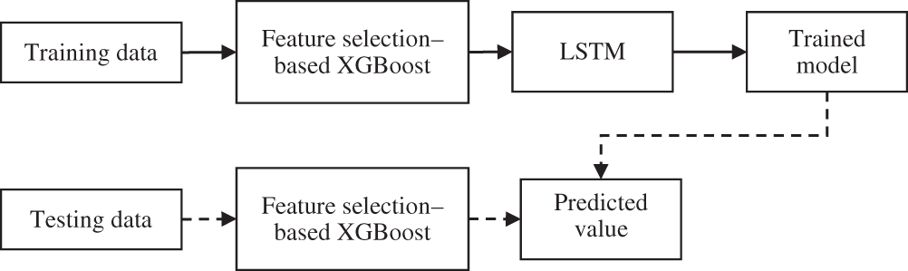
Figure 1: Block diagram of the proposed SPF method

XGBoost [28,29] is a robust machine learning algorithm for structured or tabular data. It can improve speed and performance based on the implementation of gradient-boosted decision trees. XGBoost is widely used for feature selection because of its high scalability, parallelization, efficiency, and speed.

Consider a dataset including N observations, D={X,Y}, where X={xi}i=1N,(xi∈Rd) and Y={yi}i=1N,(yi∈R) denote the training features and the observed value/target, respectively. We assume there are K numbers of gradient-boosting iterations, and M additive functions are used to predict the output. Assume y^i denotes the prediction value of the ith feature vector at the mth boost, fm , as an independent tree structure, q, with leaf weight ω (ωj represents the score on the jth leaf in the tree). Given an input feature vector xi , we computed the final predicted output by summing up the scores across all leaves as follows:

y^i=∑m=1M⁡fm(xi),fm∈F, (2)

where F={f(x)=ωq(x)} (q:ℝd→T, ω∈ℝT)  denotes the space of regression trees, q denotes the structure of each tree that maps an input to the corresponding leaf index, and T represents the number of leaves in the tree. The idea of gradient boosting is to minimize the objective function (or loss function) as follows:

Lm=∑i=1N⁡l(yi,y^i), (3)

where l denotes the difference between prediction y^i and target yi . While calibrating the gradient-boosting model, some hyperparameters related to the tree structures (e.g., subsample, max leaves, max depth) were considered to reduce overfitting. Furthermore, to reduce the model’s adaptation rate for the training dataset, the learning rate or shrinkage factor was added to the model. Adding a penalty factor or regularization term, Ω(fm) , that penalizes the model’s complexity to the objective function in Eq. (3), the generalized objective function of XGBoost is described as follows:

Lm=∑i=1N⁡l(yi,y^i)+∑m=1M⁡Ω(fm). (4)

We fed the selected features based on XGBoost into the LSTM model for SPF. The LSTM model is an extension of RNN, reducing the effect of the vanishing gradient problem. The model significantly captures contextual information within a sequence or series; it can also capture the information of a sequence output based on past and future contexts. Note that the model is executable on sequences of arbitrary lengths. It learns the long dependencies of the inputs, captures important features from the inputs, and preserves the information over a long period.

Fig. 2 illustrates the structure of a basic LSTM unit for calculating cells. A standard LSTM unit comprises a memory cell, an input gate, an output gate, and a forget gate. The past information stored in the memory cell is as important as future information. The input and output gates allow the cell to store and retrieve information over long periods. The input gate decides whether to add new information to the memory; the output gate decides what part of the LSTM unit memory contributes to the output. The forget gate is used to clear memory in the cell. Since this gate decides which information is discarded from memory, it properly captures the long-term dependency that occurs in time series.

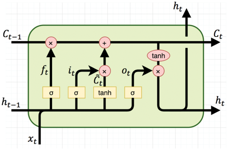
Figure 2: A basic LSTM unit

Given a frame xt in the feature sequence x = x1,…,xT, each time the LSTM unit receives xt into the sequence, it updates the hidden state, ht, with a nonlinear function that takes both current input xt and previous state ht-1. Specifically, given frame xt at current state t, ht-1 is the hidden state at previous state t-1, and ct-1 is the cell state at previous state t-1. The LSTM first calculates the forget gate ft, the input gate it, the output gate ot, and the candidate context ct~ as follows:

ft=σg([xt;ht−1]Wf+bf), (5)

it=σg([xt;ht−1]Wi+bi), (6)

ot=σg([xt;ht−1]Wo+bo), (7)

ct~=σc([xt;ht−1]Wc~+bc~), (8)

where W and b are the weight matrices and bias vector parameters, respectively, that need to be learned during training. Parameter σg is a sigmoid function while σc is a hyperbolic tangent function. Then, the cell state ct and hidden state ht at current time t are determined as follows:

ct=ft∘ct−1+it∘ct~, (9)

ct=ot∘σh(ct), (10)

where ∘ denotes the Hadamard product (element-wise product), and σh is the hyperbolic tangent function. The LSTM model is directional and is used to reflect the temporal nature of the input time series; it helps to fully exploit future contextual information. Given the higher stochasticity of financial time-series data, deep LSTMs capture more stochasticity within stock prices because of their more complex structure. Fig. 3 shows the architecture of the deep LSTM model for SPF.

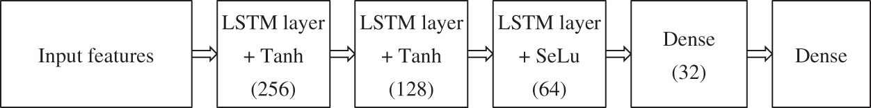
Figure 3: Architecture of deep LSTM model for SPF

3  Experimental Results

3.1 Dataset

We evaluated our proposed method using a dataset collected from the Forex market [30]. The dataset contains information covering 01/01/2008 to 03/19/2018 and has 709,314 total observations. Forex is different from the stock market because of its unique global market characteristics. A price may remain unchanged without a single trade for several minutes, or even hours, and then move dramatically as people start to trade more frequently. The Forex dataset contains a bid price of EUR/USD, and each 5 min price has over 200 features, including pricing, volatility, and volume information.

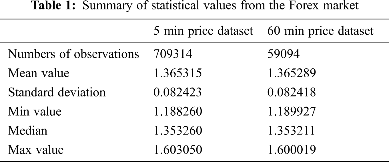
Tab. 1 shows a summary of the statistical values of the Forex market. We used closing price as the prediction target. We chose a subset of 59,094 observations with the 60 min price from the original dataset to evaluate the ARIMA model’s performance. The original dataset was used to assess the performance of the LSTM model.

3.2 Parameter Analysis

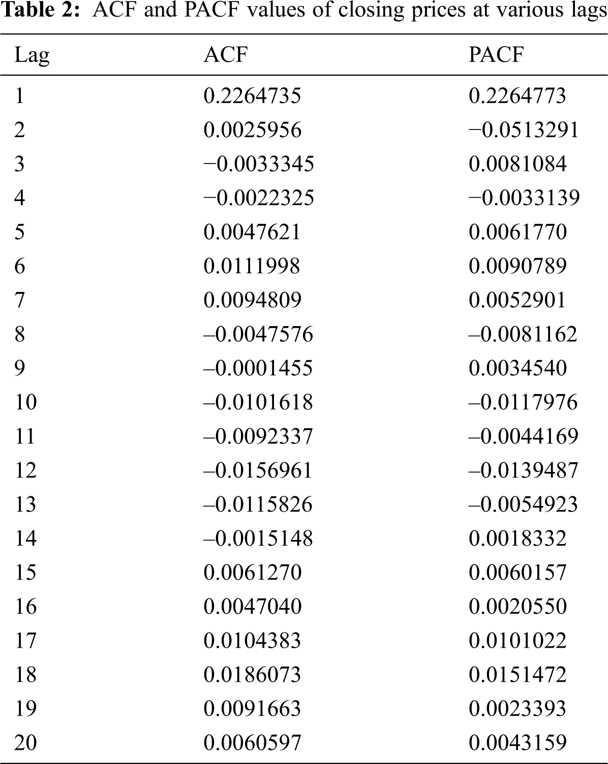
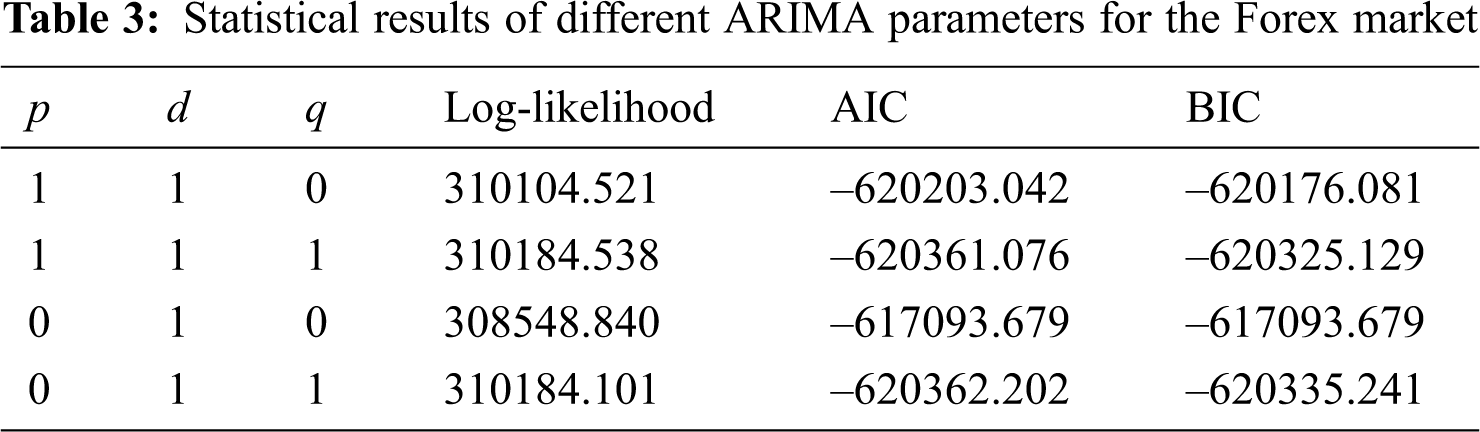
We randomly split the subdataset into two groups—approximately 70% for training and 30% for testing—to analyze the ARIMA model. Specifically, 41,365 observations were used as training data and 17,729 as test data. The training data were used to find the best parameters (p, d, q) for the ARIMA model. We used the augmented Dickey–Fuller test to determine d and found that the observations were stationary at d = 1. We also used ACF, PACF, and some criteria such as log-likelihood, BIC, and AIC to determine p and q. Tab. 2 shows the ACF and PACF values of the closing prices from the training data at various lags. Additionally, Tab. 3 presents the statistical results of different ARIMA parameters for the Forex market. We chose the best model based on minimum BIC and AIC values and maximum log-likelihood values. Therefore, the ARIMA (0,1,1) was considered the best model for the Forex market.

In the XGBoost and LSTM approaches, we randomly split the original dataset into three groups: approximately 60% for training, 20% for validation, and 20% for testing. We used 397,216 observations for training, 170,235 observations for validation, and 141,863 observations for testing. The observations were high-dimensional data with 200 features. We used XGBoost to select feature importance based on the F-score value. Fig. 4 presents some important features selected based on XGBoost. We realized that 10 important features selected from XGBoost and fed into the LSTM model gave the best accuracy. We used Adam optimization as an optimizer and 50 epochs to train the LSTM model in Keras.

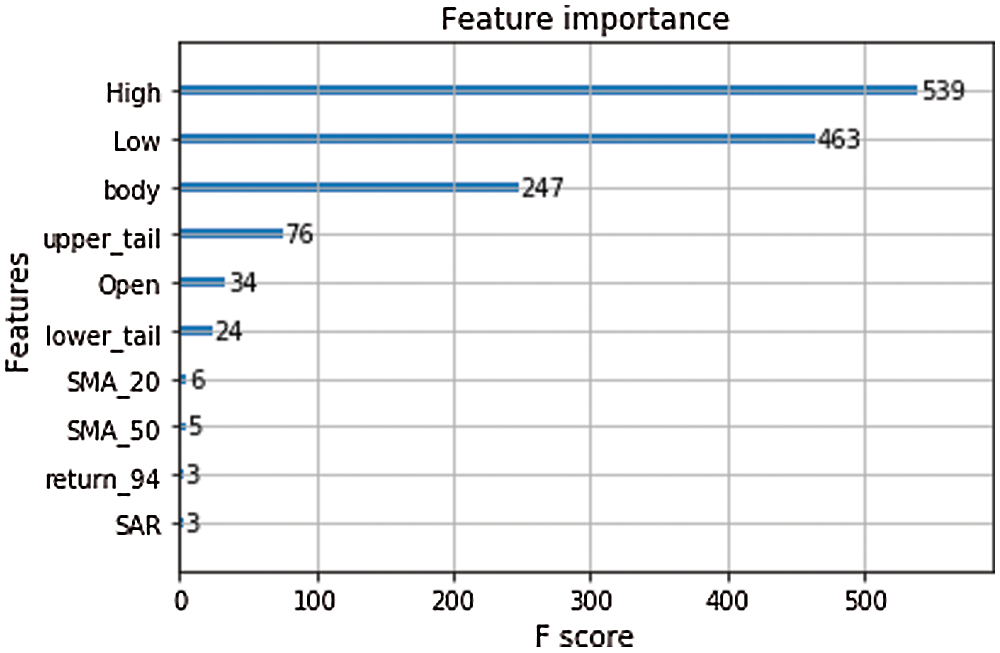
Figure 4: Selected important features based on XGBoost

Finally, we used MAE, MSE, and RMSE as the metrics to evaluate the accuracy of the SPF system. The lower the values, the more accurate the system.

3.3 Results

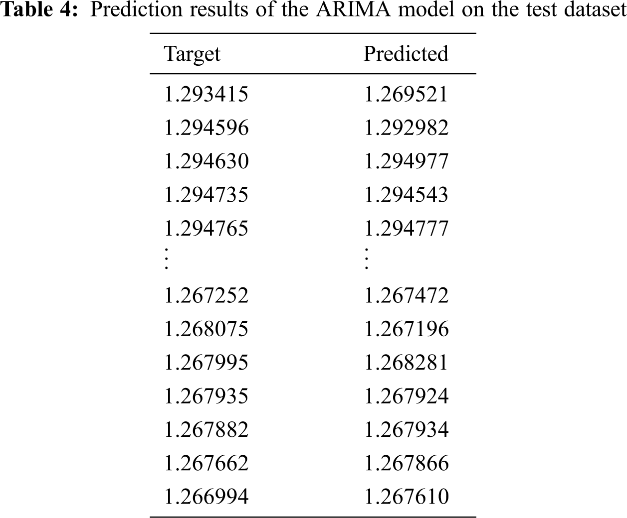
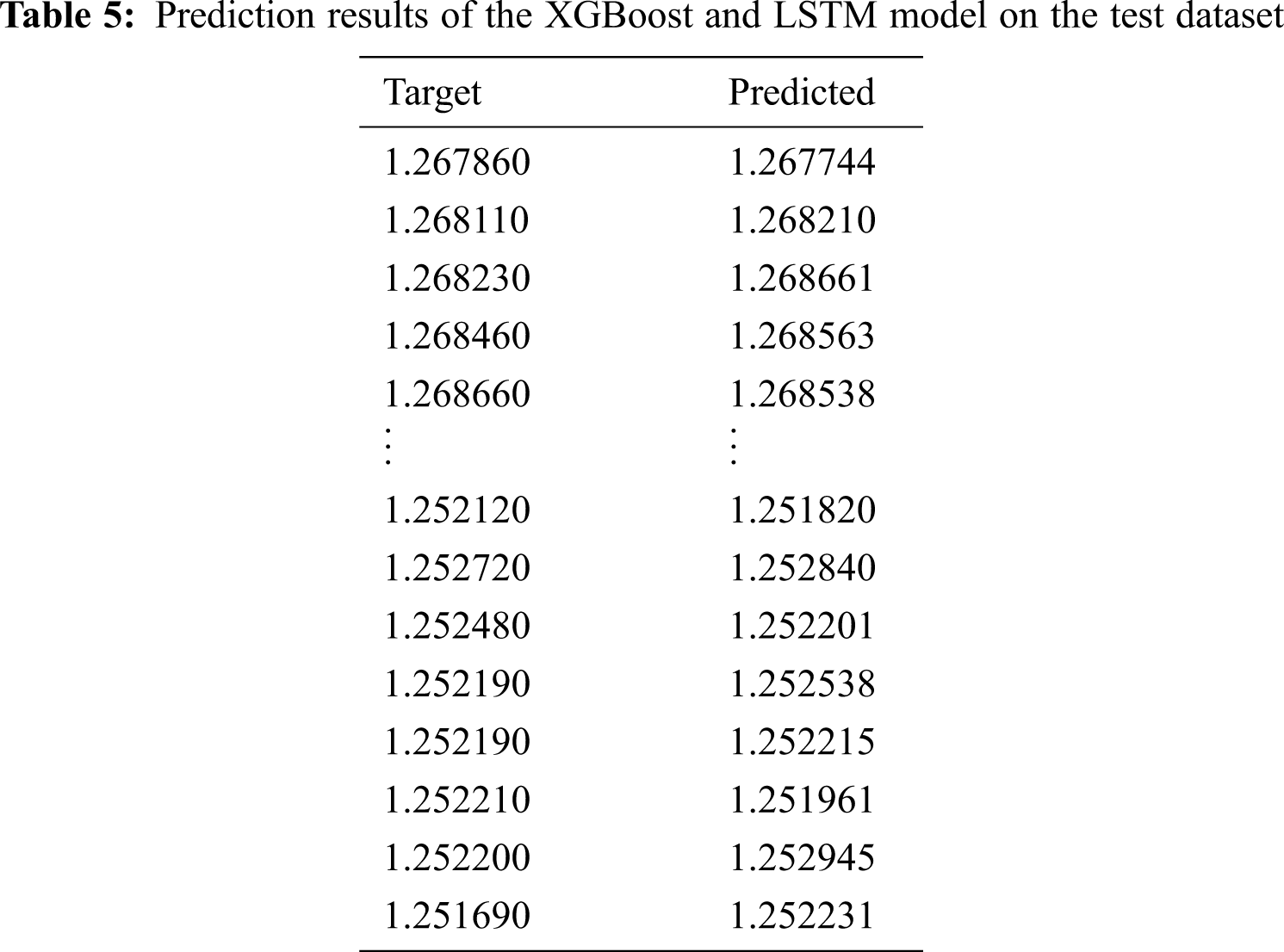
Tabs. 4 and 5 show the prediction results of the ARIMA model and our approach for the test dataset. The predicted closing price values obtained using both approaches were very close to the target values. Therefore, both the ARIMA model and our approach yielded high forecasting accuracy.

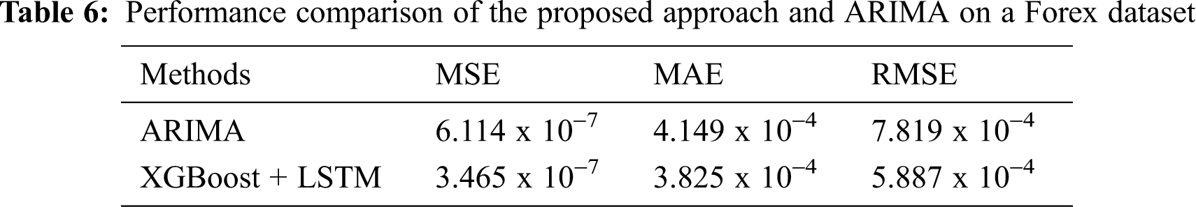
Tab. 6 presents a comparison of the performance of our approach and the baseline ARIMA approach. It shows that the proposed approach performed better than the ARIMA model and achieved the best accuracy. As for long-term time-series prediction, the LSTM model has the advantage of selecting important and relevant information, thereby enhancing predictive performance. Therefore, our proposed approach can be considered a promising method for improving the accuracy of SPF.

4  Conclusion

This study proposed an improved SPF system by combining XGBoost and LSTM models. We first introduced the construction of important features from a high-dimensional dataset using XGBoost as the feature-selection method. Then, the features were fed into deep LSTM models to evaluate the performance of the forecasting system. The experimental results verified that the proposed approach significantly improved the accuracy of the SPF system and outperformed the baseline ARIMA approach.

Funding Statement: The authors received no specific funding for this study.

Conflicts of Interest: The authors have no conflicts of interest to declare regarding this study.

References

 1.  Z. Hu, Y. Zhao and M. Khushi, “A survey of Forex and stock price prediction using deep learning,” Applied System Innovation, vol. 4, no. 9, pp. 1–30, 2021. [Google Scholar]

 2.  H. Hewamalage, C. Bergmeir and K. Bandara, “Recurrent neural networks for time series forecasting: Current status and future directions,” International Journal of Forecasting, vol. 37, no. 1, pp. 388–427, 2021. [Google Scholar]

 3.  A. A. Ariyo, A. O. Adewumi and C. K. Ayo, “Stock price prediction using the ARIMA model,” in 2014 UKSim-AMSS 16th Int. Conf. on Computer Modelling and Simulation, IEEE, pp. 106–112, 2014. [Google Scholar]

 4.  P. Mondal, L. Shit and S. Goswami, “Study of effectiveness of time series modeling (ARIMA) in forecasting stock prices,” International Journal of Computer Science, Engineering and Applications, vol. 4, no. 2, pp. 13–29, 2014. [Google Scholar]

 5.  J. E. Jarrett and E. Kyper, “ARIMA modeling with intervention to forecast and analyze Chinese stock prices,” International Journal of Engineering Business Management, vol. 3, no. 3, pp. 53–58, 2011. [Google Scholar]

 6.  S. Mishra, “The quantile regression approach to analysis of dynamic interaction between exchange rate and stock returns in emerging markets: Case of BRIC nations,” IUP Journal of Financial Risk Management, vol. 13, no. 1, pp. 7–27, 2016. [Google Scholar]

 7.  K. J. Lee, A. Y. Chi, S. Yoo and J. Jongdae Jin, “Forecasting Korean stock price index (KOSPI) using back propagation neural network model, Bayesian Chiao’s model, and SARIMA model,” Academy of Information & Management Sciences Journal, vol. 11, no. 2, pp. 32–35, 2008. [Google Scholar]

 8.  Z. Zeng and M. Li, “Bayesian median autoregression for robust time series forecasting,” International Journal of Forecasting, vol. 7, no. 2, pp. 1000–1010, 2021. [Google Scholar]

 9.  M. C. Tsai, C. H. Cheng, M. I. Tsai and H. Y. Shiu, “Forecasting leading industry stock prices based on a hybrid time-series forecast model,” PLoS One, vol. 13, no. 12, pp. 1–24, 2018. [Google Scholar]

10. M. Ballings, D. V. D. Poel, N. Hespeels and R. Gry, “Evaluating multiple classifiers for stock price direction prediction,” Expert Systems with Applications, vol. 42, no. 20, pp. 7046–7056, 2015. [Google Scholar]

11. J. Zhang, S. Cui, Y. Xu, Q. Li and T. Li, “A novel data-driven stock price trend prediction system,” Expert Systems with Applications, vol. 97, pp. 60–69, 2018. [Google Scholar]

12. F. Yang, Z. Chen, J. Li and L. Tang, “A novel hybrid stock selection method with stock prediction,” Applied Soft Computing, vol. 80, pp. 820–831, 2019. [Google Scholar]

13. S. Selvin, R. Vinayakumar, E. A. Gopalakrishnan, V. K. Menon and K. P. Soman, “Stock price prediction using LSTM, RNN and CNN-sliding window model,” in 2017 Int. Conf. on Advances in Computing, Communications and Informatics (ICACCIUdupi, India: IEEE, pp. 1643–1647, 2017. [Google Scholar]

14. E. Hoseinzade and S. Haratizadeh, “CNNpred: CNN-based stock market prediction using a diverse set of variables,” Expert Systems with Applications, vol. 129, pp. 273–285, 2019. [Google Scholar]

15. M. Wen, P. Li, L. Zhang and Y. Chen, “Stock market trend prediction using high-order information of time series,” IEEE Access, vol. 7, pp. 28299–28308, 2019. [Google Scholar]

16. M. Nabipour, P. Nayyeri, H. Jabani, A. Mosavi and E. Salwana, “Deep learning for stock market prediction,” Entropy, vol. 22, no. 8, pp. 1–23, 2020. [Google Scholar]

17. R. Singh and S. Srivastava, “Stock prediction using deep learning,” Multimedia Tools and Applications, vol. 76, no. 18, pp. 18569–18584, 2017. [Google Scholar]

18. H. Maqsood, I. Mehmood, M. Maqsood, M. Yasir, S. Afzal et al., “A local and global event sentiment based efficient stock exchange forecasting using deep learning,” International Journal of Information Management, vol. 50, pp. 432–451, 2020. [Google Scholar]

19. W. Long, Z. Lu and L. Cui, “Deep learning-based feature engineering for stock price movement prediction,” Knowledge-Based Systems, vol. 164, pp. 163–173, 2019. [Google Scholar]

20. S. Siami-Namini, N. Tavakoli and A. S. Namin, “A comparison of ARIMA and LSTM in forecasting time series,” in 2018 17th IEEE Int. Conf. on Machine Learning and Applications (ICMLAOrlando, FL, USA: IEEE, pp. 1394–1401, 2018. [Google Scholar]

21. S. Mehtab, J. Sen and A. Dutta, “Stock price prediction using machine learning and LSTM-based deep learning models,” In: S. M. Thampi, S. Piramuthu, KC. Li, S. Berretti, M. Wozniak, D. Singh (eds.Machine Learning and Metaheuristics Algorithms, and Applications. SoMMA 2020. Communications in Computer and Information Science, vol. 1366, pp. 88–106, 2021. [Google Scholar]

22. S. Siami-Namini, N. Tavakoli and A. S. Namin, “A comparative analysis of forecasting financial time series using ARIMA, LSTM, and BiLSTM,” arXiv preprint arXiv:1911.09512, 2019. [Google Scholar]

23. W. Chen, C. K. Yeo, C. T. Lau and B. S. Lee, “Leveraging social media news to predict stock index movement using RNN-boost,” Data & Knowledge Engineering, vol. 118, pp. 14–24, 2018. [Google Scholar]

24. Y. Baek and H. Y. Kim, “ModAugNet: A new forecasting framework for stock market index value with an overfitting prevention LSTM module and a prediction LSTM module,” Expert Systems with Applications, vol. 113, pp. 457–480, 2018. [Google Scholar]

25. T. Fischer and C. Krauss, “Deep learning with long short-term memory networks for financial market predictions,” European Journal of Operational Research, vol. 270, no. 2, pp. 654–669, 2018. [Google Scholar]

26. Z. Jin, Y. Yang and Y. Liu, “Stock closing price prediction based on sentiment analysis and LSTM,” Neural Computing and Applications, vol. 32, pp. 9713–9729, 2020. [Google Scholar]

27. X. Li, P. Wu and W. Wang, “Incorporating stock prices and news sentiments for stock market prediction: A case of Hong Kong,” Information Processing & Management, vol. 57, no. 5, pp. 1–19, 2020. [Google Scholar]

28. T. Chen and C. Guestrin, “XGBoost: A scalable tree boosting system,” in Proc. of the 22nd ACM SIGKDD Int. Conf. on Knowledge Discovery and Data Mining, pp. 785–794, 2016. [Google Scholar]

29. Y. Wang and X. S. Ni, “A XGBoost risk model via feature selection and Bayesian hyper-parameter optimization,” International Journal of Database Management Systems (IJDMS), vol. 11, no. 1, pp. 1–10, 2019. [Google Scholar]

30. Forex market dataset, “2019 International Data Science Competition,” 2019. [Online]. Available at: https://www.isods.org/news-times/item/1-2019-international-data-science-competition. [Google Scholar]

This work is licensed under a Creative Commons Attribution 4.0 International License, which permits unrestricted use, distribution, and reproduction in any medium, provided the original work is properly cited.