Computer Systems Science & Engineering DOI:10.32604/csse.2022.017484
Article

Ensemble Classifier Technique to Predict Gestational Diabetes Mellitus (GDM)

A. Sumathi* and S. Meganathan

SRC, SASTRA Deemed to be University, Kumbakonam, Tamil Nadu, 612001, India
*Corresponding Author: A. Sumathi. Email: sumathi@src.sastra.edu
Received: 31 January 2021; Accepted: 23 April 2021

Abstract: Gestational Diabetes Mellitus (GDM) is an illness that represents a certain degree of glucose intolerance with onset or first recognition during pregnancy. In the past few decades, numerous investigations were conducted upon early identification of GDM. Machine Learning (ML) methods are found to be efficient prediction techniques with significant advantage over statistical models. In this view, the current research paper presents an ensemble of ML-based GDM prediction and classification models. The presented model involves three steps such as preprocessing, classification, and ensemble voting process. At first, the input medical data is preprocessed in four levels namely, format conversion, class labeling, replacement of missing values, and normalization. Besides, four ML models such as Logistic Regression (LR), k-Nearest Neighbor (KNN), Support Vector Machine (SVM), and Random Forest (RF) are used for classification. In addition to the above, RF, LR, KNN and SVM classifiers are integrated to perform the final classification in which a voting classifier is also used. In order to investigate the proficiency of the proposed model, the authors conducted extensive set of simulations and the results were examined under distinct aspects. Particularly, the ensemble model has outperformed the classical ML models with a precision of 94%, recall of 94%, accuracy of 94.24%, and F-score of 94%.

Keywords: GDM; machine learning; classification; ensemble model

1  Introduction

Gestational Diabetes Mellitus (GDM) is a disease characterized by fluctuating glucose levels in blood during pregnancy [1]. One of the recent findings infer that Chinese women suffer from GDM during their pregnancy and it is progressing rapidly across the globe. Mothers with GDM are subjected to metabolic interruption, placental dysfunction, progressive risks for preeclampsia and cesarean delivery. Hyperglycemia and placental dysfunction result in less fetal growth and high risks of birth trauma, macrosomia, preterm birth, and shoulder dystocia [2]. Followed by, a mother with GDM and the newborn baby experience post-partum complications including obesity, type 2 DM, and heart attack. Earlier prognosis and prevention are highly important to reduce the prevalence of GDM and low adverse pregnancy [3]. But, most of the GDM cases are diagnosed between 24th and 28th weeks of pregnancy through Oral Glucose Tolerance Test (OGTT). This is an accurate window for intervention, since fetal and placental growth pre-exist at this point.

The study conducted earlier [4] recommended OGTT diagnosis method at early stages of pregnancy itself. However, it is expensive and ineffective in most of the scenarios since GDM manifests during mid-to-late delivery. Therefore, a simple model should be introduced with the help of traditional medical information at earlier pregnancy. This model should help in measuring the risks of GDM and find high-risk mothers who require earlier treatment, observation, and medications. This way, universal OGTTs can be reduced among low-risk women. The detection methods that were recently developed to predict GDM is deployed with the help of classical regression analysis. But, Machine Learning (ML), a data analytics mechanism, creates the model for predicting results by ‘learning’ from the data. This approach has been emphasized as a competent replacement for regression analysis. Furthermore, ML is capable of performing well than the traditional regression, feasibly by the potential of capturing nonlinearities and complicated interactions between predictive attributes [5]. Though maximum number of studies have been conducted earlier in this domain, only limited works have applied ML in the prediction of GDM, and no models were compared with Logistic Regressions (LR).

Xiong et al. [6] decided to develop the first 19 weeks’ risk prediction mechanism with high-potential GDM predictors using Support Vector Machine (SVM) and light Gradient Boosting Machine (light GBM). Zheng et al. [7] presented a simple approach to detect GDM in earlier pregnancy using biochemical markers as well as ML method. In the study conducted by Shen et al. [8], it was mentioned that the investigation of optimal AI approach in GDM prediction requires minimal clinical devices and trainees so as to develop an application based on Artificial intelligence (AI). In the literature [9], the prediction of GDM using different ML approaches is projected on PIMA dataset. Hence, the accuracy of ML models was validated using applied performance metrics. The significance of the ML technique is understood through confusion matrix, Receiver Operating Characteristic (ROC), and AUC measures in the management of diabetes PIMA data set. In Srivastava et al. [10], a statistical framework was proposed to estimate GDM using Microsoft Azure AI services. It is referred to as ML Studio with optimal performance and use drag and drop method. Further, this study also used a classification model to forecast the presence of GDM according to the factors involved during earlier phases of pregnancy. The study considered Cost-Sensitive Hybrid Model (CSHM) and five conventional ML approaches to develop the prediction schemes.

The authors in the literature [11] has examined the future risks of GDM through temporary Electronic Health Records (EHRs) [11]. After the completion of data cleaning process, few data has to be recorded and collected for constructing the dataset. In literature [12], the authors developed an artificial neural network (ANN) method called Radial Basis Function Network (RBF Network) and conducted performance validation and comparison analysis. This method was employed to identify the possible cases of GDM which may develop multiple risks for pregnant women and the fetus. In Ye et al. [13], parameters were trained using diverse ML and conventional LR methodologies. In Du et al. [14], three distinct classifiers were employed to predict the risk of GDM in future. The detection accuracy in this study helps the clinician to make optimal decisions and accordingly the disease is prevented easily. The study found that DenseNet model was able to detect the GDM with maximum flexibility.

The current research paper introduces an ensemble of ML-based GDM prediction and classification models. The presented model involves three processes such as preprocessing, classification, and ensemble voting process. For classification, four ML models such as Logistic Regression (LR), k-Nearest Neighbor (KNN), Support Vector Machine (SVM), and Random Forest (RF) were used by the researcher. Moreover, RF, LR, and SVM classifiers were integrated to perform the final classification in which a voting classifier was also used. To validate the proficiency of the proposed method, the results of the analysis attained from the presented model was compared with traditional methods. Further, a widespread set of experimentations was also conducted on different aspects.

2  The Proposed Model

The working principle of the presented model is depicted in Fig. 1. As shown in the Figure, the input medical data is initially preprocessed in four levels namely format conversion, class labeling, normalization, and missing value replacement. Then, the preprocessed data is fed into the ML models to determine the proper class label. At last, the ensemble model is applied to determine the appropriate class labels of the applied data instances. The detailed working of the preprocessing, ML, and ensemble models are defined in the subsequent subsections.

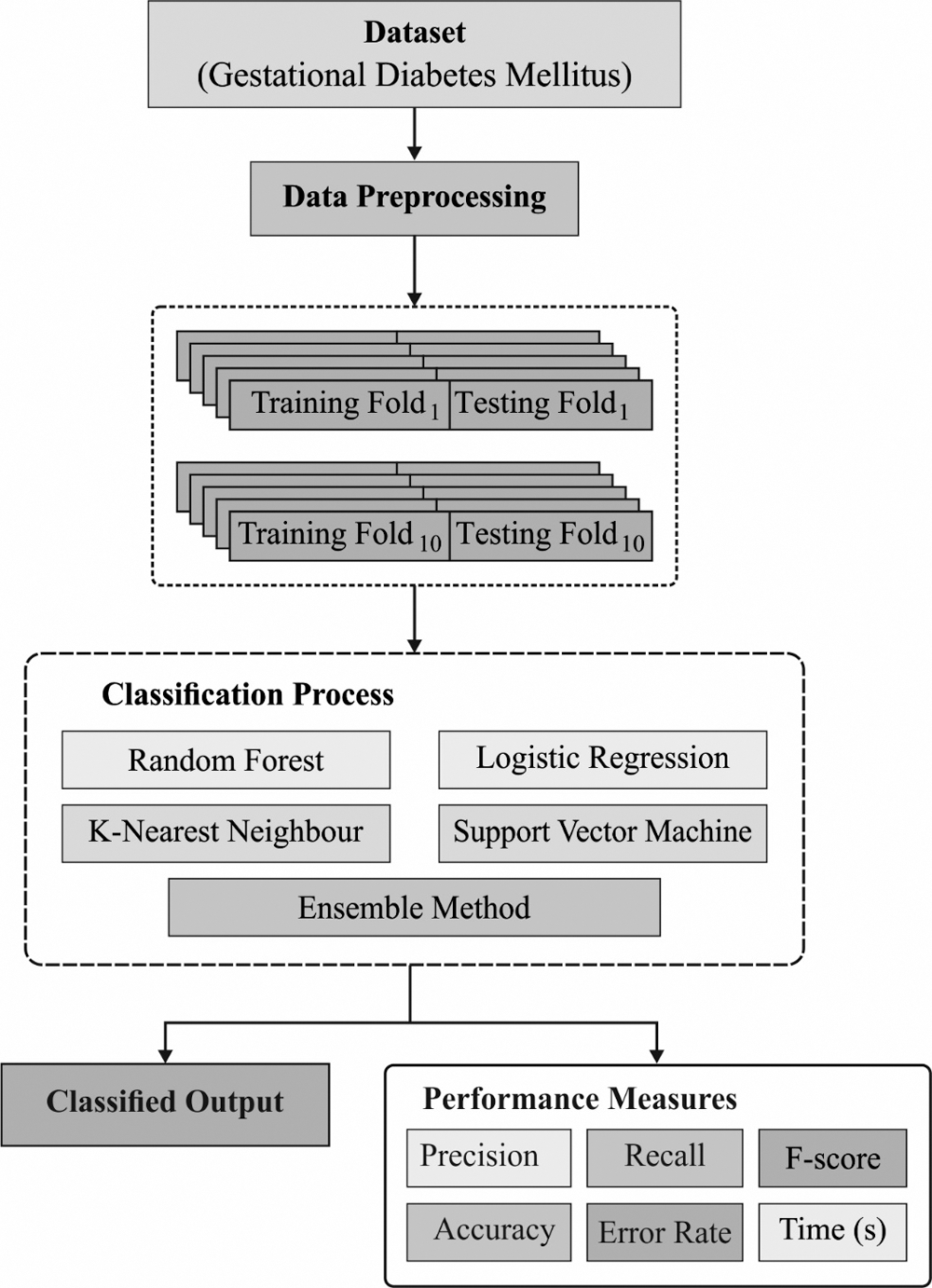
Figure 1: Working process of the proposed method

2.1 Data Pre-Processing

In this stage, input clinical data is pre-processed to enhance the quality of data in different ways. Initially, data conversion is carried out from input data (.xls type) which is transformed to .csv format. Followed by, class labeling task is performed during when the data samples are assigned to respective class labels. Then, min-max model is employed for data normalization task. At this point, maximum and minimum values are taken from the collected data while the remaining data is normalized for these measures. The main aim of this scheme is to normalize the data instances to a minimum value of 0 and a maximum value of 1. Eq. (2) provides min-max normalization function.

Min−Max.Norm=x−xminxmax−xmin (1)

Besides, the missing values are replaced with the help of group-based mean concept. It is a general transformation in statistical analysis with collective data which replaces the missing data inside a group with mean value of non-NaN measures in a group.

2.2 Classification Models

In this stage, the preprocessed input data is fed as input to the ML model so as to identify the class label properly.

2.2.1 Logistic Regression

LR is a type of regression mechanism applied in the prediction of possibilities of GDM and corresponding features, which depend upon any class of explanatory parameters like continuous, discrete, or categorical. Since the predicted possibility should exist between 0 and 1, simple linear regression model is adequate for accomplishing the accurate GDM detection. This is because it enables the dependent variable to pass limits and generates negative outcomes. As defined in P1 , the possibility of an object falls under group 1, and P0 denotes the probability of an object from group 0 . LR method is given herewith.

zi=log(Pi1Pi0)=b0+b1xi1+b2xi2+⋯+bkxik, (2)

where Pi1/Pi0 defines the odd ratio, bj refers to the value of jth coefficient, =1, k , and xij imply the value of ith case of the jth predictor. The parameters ( bo to bk ) of logistic mechanism are evaluated using high likelihood concept [15]. The possibility of an event, to be prevalent, is evaluated with the help of LR framework given below.

P(Yi=1/Xi)=ebTX;1+(ebTXi)=11+e−bTXi, (3)

where ebTXi denotes the linear predictor of LR function, and Yi indicates a dependent variable.

When the probability cutoff of 0.5 is applied, classification is performed from object to group 1, while at the same time, P1 > 5 and group 0 are estimated if P1 < 5 . To evaluate the parameters of LR approach, maximum likelihood enhances the coefficients of log− likelihood function, and the statistics consolidates the data of predictor variables. Both logistic and linear discriminant regression analysis are composed of similar functional frame i.e., a mixture of autonomous variables and a principle for classification. However, massive differences exist in the assumptions made to be applied in a dataset.

2.2.2 K-Nearest Neighbor (KNN)

KNN classifier is one of the simple and effective ML methods. Here, an object is divided based on majority vote of the neighbors. As a result, the object is allocated to a class using KNN prominently. Here, K defines a positive integer with a small value. When K = 1 , then the object is simply allocated to a class of the nearest neighbor.

Initially, KNN is developed by few expressions =(xi,yi) where j=1,2,...N is assumed to be the training set, xi defines the d -dimensional feature vector, and yi∈{+1,−1} depicts the observed class labels. Followed by, binary classification was applied in this study [16]. Generally, training data has iid samples of random parameters (X,Y) with symmetric distribution.

Under the application of previously-labeled instances as training set S , KNN approach develops a local subregion R(x)⊆ℜd of input space, which is then placed at evaluation point, x . Hence, the predicting region R(x) is comprised of nearby training which points at x and is demonstrated as given below:

R(x)={x^|D(x,x^)≤d(k)}, (4)

where d(k) denotes the kth order statistic of {D(x,x^)}1N , whereas D(x,x^) defines the distance measure. k[y] refers to the number of samples in region R(x) and is named after y . Also, KNN is statistically developed to evaluate the posterior possibility p(y|x) of observation point, x :

p(y|x)=p(x|y)p(y)p(x)≅k[y]k. (5)

For applied observation x , decision g(x) is developed by measuring the scores of k[y] and selecting the class with maximum k[y] value.

g(x)={1,k[y=1]≥k[y=−1],−1,k[y=−1]≥k[y=1]., (6)

Hence, the decision that enhances the relevant posterior probability is applied in KNN method. For binary classification issues, where yi∈{+1,−1} , KNN mechanism generates the decision rule as shown below:

g(x)=sgn(avexi∈R(x)yi) (7)

2.2.3 Support Vector Machine

SVM resolves the pattern classification and regression issues. Recently, SVM method has gained reasonable attention from the developers, thanks to its maximum generalization ability. It is extensively applied since it exhibits optimal performance in comparison with classical learning machines. The major responsibility of SVM is to identify the separating hyperplane that classifies the data points into two categories. Assume a binary classifier with l training instances {(x1,y1),(x2,y2),(xl,yl)} , where xi=(xi1,xi2,…,xid)T implies a d -dimensional data point as well as yi∈{+1,−1} refers to class label. Hence, a decision boundary of linear classification method is illustrated as shown below.

w⋅x+b=0, (8)

where w and b imply the parameters of a scheme. In order to overcome the nonlinearly-separable data, the training samples should be converted into high-dimensional feature space under the application of nonlinear mapping, Φ . Thus, the Eq. (8) is modified as shown herewith.

The concept of SVM needs a better solution for optimization issue.

minw‖w‖22 (9)

Subjected to yi(w⋅Φ(xi)+b)≥1 , for j=1,…,l.

The optimization problem can be resolved by developing a Lagrangian demonstration and incorporating it into a dual problem:

LD=∑i=1l⁡αi−12∑i=1l⁡∑j=1l⁡αiαjyiyjΦ(xi)⋅Φ(xj). (10)

When αi is identified with the help of quadratic programming model [17], then KKT conditions are used in the depiction of the best variable w by means of best dual variables based on w = ∑i=1l⁡αiyiΦ(xi) . It is pointed out that w is based on xi for αi≠0 , which is referred to as Support Vectors (SVs). Fig. 2 illustrates the hyperplanes of SVM model.

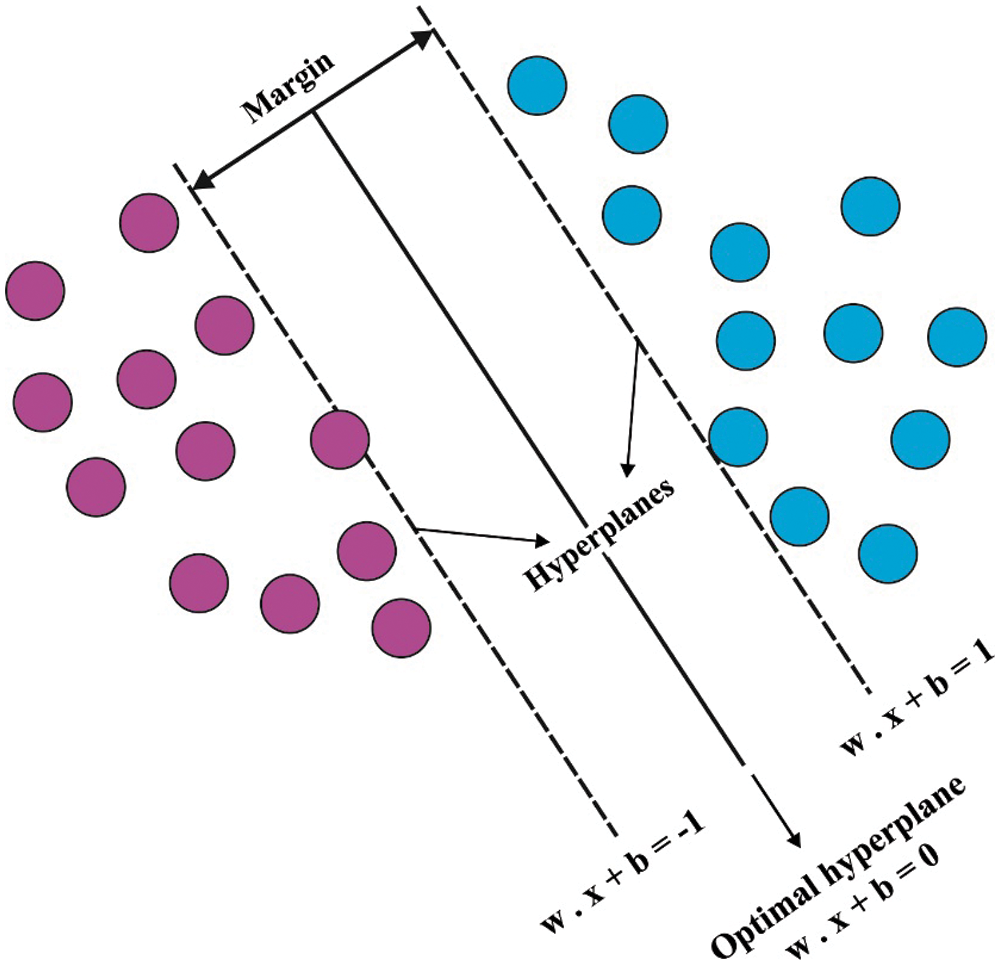
Figure 2: Hyper planes of SVM model

If optimal pair (w0,b0) is computed, then SVM decision function is depicted as given herewith.

f(x)=sign(∑i∈SVs⁡αiyiΦ(xi)⋅Φ(x)+b). (11)

If f(x)=1 , then a test sample x is divided into positive class; or else, it is placed under negative class.

Moreover, a dot product Φ(xi)⋅Φ(xj) from the transformed space is represented as a kernel function K(xi,xj) = Φ(xi)⋅Φ(xj) . Hence, a kernel is defined as a major objective to be used in the validation of SVM performance. Different kernel functions are used in linear kernel (xi,xj)= xi⋅xj , a polynomial kernel K(xi,xj)=(axiTxj+r)d and RBF kernel K(xi,xj)=exp(−γ‖xi−xj‖2) .

2.2.4 Random Forest

RF is defined as an ensemble of learning classifier and regression model and is applied in handling the issues faced during data collection within a class. In RF, detection process is computed by Decision Trees (DT). In case of training phase, numerous DTs are developed and employed for class prediction. This task is accomplished by assuming the voted categories of trees and class with the maximum vote which is otherwise referred to as simulation outcome.

RF approach was already employed to resolve the issues projected in this study [18]. Here, the classification method is trained and the samples are applied after 10-fold cross-validation. Here, the dataset is classified into ten different portions out of which 9 are applied in training process. The details accomplished during training phase might be employed for testing process too. Therefore, cross-validation ensures that the training data is different from testing data. In ML, this model is referred to as the supreme estimate of generalization error.

2.3 Ensemble Classifier

Ensemble classification method is a combination of different single classifiers which perform similar processes to enhance the efficiency of classification (the discriminant ability of complete model). This scenario is considered to be an accurate assignment of the objects. This combination is achieved by aggregating the classifier outcomes gained from component classification method and is done to construct a final classifier with optimal prediction capabilities. To identify GDM, three classifiers namely LR, RF, and KNN are employed in this study. The basic concept is to unify the simulation outcomes to accomplish consequent classification. This model is capable of enhancing the classification result attained from GDM dataset. Also, it is operated with an Ensemble Vote Classifier. It enables reduced outcomes of different disorders, where the scalable solution is processed with ‘irregular data’.

At this point, group G of N classifiers are considered under less complex base classifiers G={C1;…;Ck};k=1…N which solely depend upon the final decision taken [19]. Some of the common modalities are given herewith.

1. Majority voting

2. Weighted majority voting

3. Robust models depend upon bagging as well as boosting principles

Assume kth decision which selects the jth class as shown below:

dkj∈{0,1};k=1,N;j=1,…,M, (12)

where N signifies the count of classifiers and M denotes the count of classes. When kth classifier selects class J , then dk;J=1 , and dk;J=0 , else. Voting-relied approaches are operated on labels in which dk.J is 1 or 0 that depends on the selection of the classifier k and if it selects J , it is 1 or else 0. Hence, the ensemble decides class J to receive the maximum vote.

In majority voting case, a consequent class label is selected as the class label predicted prominently by single classifiers. It is a simple case of ensemble voting mechanism. Thus, the decision DG is given below.

DG=argmaxj=1,…,M∑k=1N⁡dk,j. (13)

Assume a set of three classification models G={C1;C2;C3} which classify an observation of two classes namely, ‘A’ or ‘B’:

C1→ class A,

C2→ class A,

C3→ class B.

The following expressions are derived from Eq. (13):

forclassA→∑k=13⁡dk,A=1+1+0=2,forclassB→∑k=13⁡dk,B=0+0+1=1. (14)

Weighted majority voting case varies from hard voting and it describes the factor ωk as the weight allocated for kth classifer Ck based on few performance metrics. Eq. (13) has a defined shape as given below.

DG=argmaxj=1,…,M∑k=1N⁡ωkdk,j. (15)

Next, consider a group of three classifiers G={C1,C2,C3} and three weights ω1,ω2,ω3 which divide the observation as given herewith.

C1→ class A and ω1 = 0.2,

C2→ class A and ω2 = 0.2,

C3→ class B and ω3 = 0.6.

Then, using (15), the following expression is accomplished,

for classA→∑k=l3⁡ωkdkA=0.2×1+0.2×1+0.6×0=0.4, (16)

for classB→∑k=l3⁡ωkdkB=0.2×0+0.2×0+0.6×1=0.6, (17)

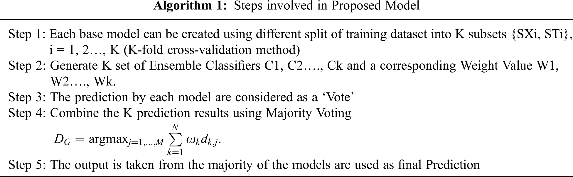
So, it is clear that the sample can be classified as ‘Class B’. It is regarded as a second mechanism to compute the optimal performance. (Algorithm format)

3  Experimental Validation

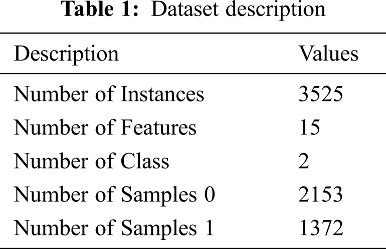
For experimentation, GDM prediction model was developed by the researcher using Python. Real-time GDM data set was fed as input to the application which performed data pre-processing initially. Then the data underwent transformation. After the development of a promising training model, it was used for prediction. The presented model was tested using GDM dataset. It is composed of 3525 instances with the existence of 15 features. In addition, the number of instances under class 0 is 2153 whereas the number of instances under class 1 is 1372. The information related to dataset is provided in Tab. 1 whereas the frequency distribution of the attributes is tabulated in Fig. 3.

Figure 3: Frequency distribution of GDM dataset

Tab. 2 provides the detailed results attained from the analysis of different ML and ensemble models in terms of dynamic performance measures. Fig. 4 shows the precision and recall analyses of different ML models on the applied GDM dataset. The figure portrays that the SVM model is an ineffective performer since it obtained the least precision of 82% and recall of 83%. Besides, the KNN model achieved slightly higher prediction outcomes with a precision of 85% and recall of 83%. In addition, the LR model attained a moderate result i.e., precision of 92% and recall of 90%. Moreover, the RF model produced a competitive precision of 93% and recall of 93%. At last, the ensemble model outperformed other ML models by achieving a precision of 94% and recall of 94%.

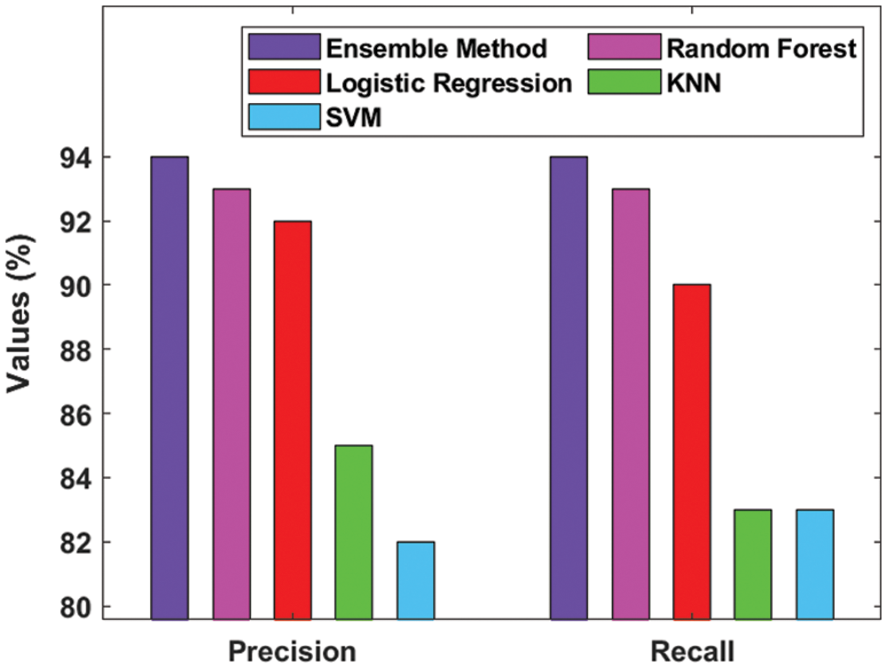
Figure 4: Results of ensemble model in terms of precision and recall

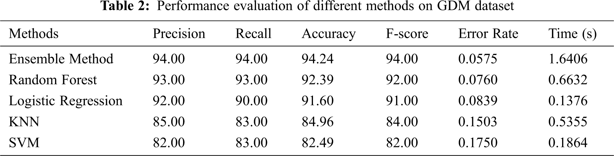
Fig. 5 inspects the accuracy and F-score analyses of diverse ML models on the applied GDM dataset. The figure depicts that the SVM model is the worst performer since it gained the least accuracy of 82.49% and an F-score of 82%. However, the KNN model yielded a slightly high prediction outcome i.e., accuracy of 84.96% and an F-score of 84%. Additionally, the LR model accomplished a reasonable result with an accuracy of 91.60% and F-score of 91%. Here, the RF model yielded a competitive accuracy of 91.60% and F-score of 92%. Further, the ensemble model has outclassed other ML models with an accuracy of 94.24% and F-score of 94%.

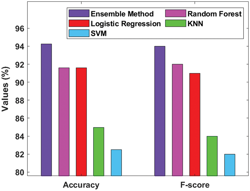
Figure 5: Result of ensemble model in terms of Accuracy and F-score

An error rate analysis of different ML and ensemble models is shown in Fig. 6. The figure states that both KNN and SVM models yielded poor results with maximum error rates of 0.1503 and 0.1750 respectively. Followed by, the LR model outperformed the KNN and SVM models with an error rate of 0.0839. Simultaneously, the RF model attempted to attain a near-optimal error rate of 0.0760. But the presented ensemble model accomplished an effective prediction outcome with a minimal error rate of 0.0575.

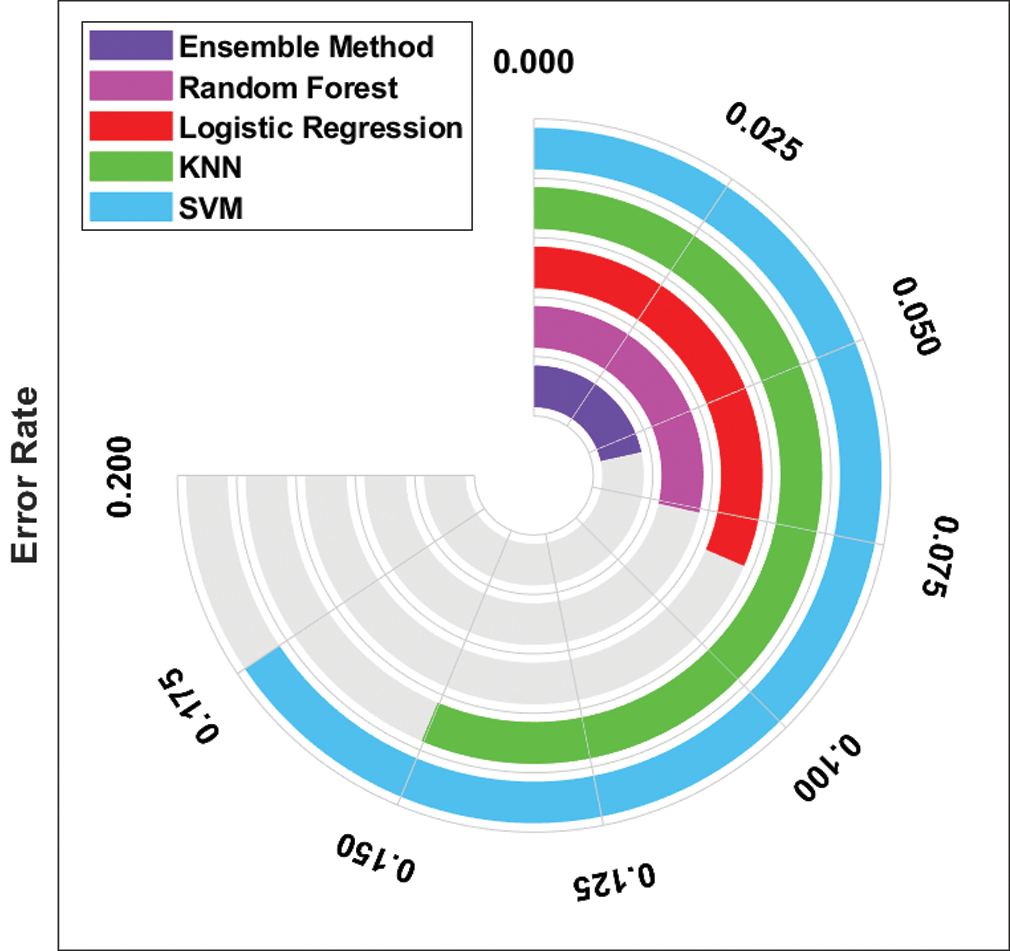
Figure 6: Error rate analysis of ensemble model

Fig. 7 shows the computation time analysis of diverse ML and ensemble models. The figure portrays that both LR and SVM models demonstrated the least computation times of 0.1376 s and 0.1864 s respectively. Concurrently, the RF and SVM models exhibited moderate computation times of 0.6632 s and 0.5355 s respectively. However, the presented ensemble model demanded a maximum computation time of 1.6406 due to the integration of multiple classifier models. Though it requires maximum computation time, the classification results of the ensemble model were considerably high than other ML models.

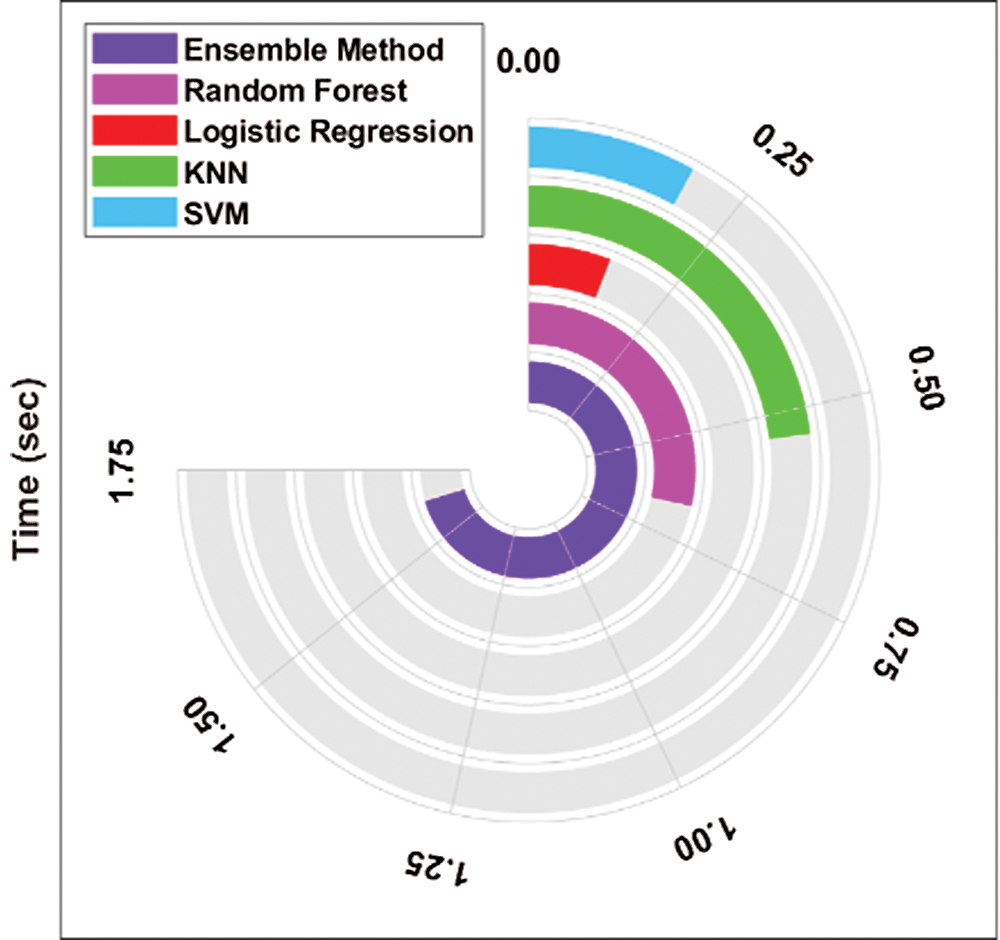
Figure 7: Computation time analysis of ensemble model

Fig. 8 shows the ROC analysis of different ML and ensemble models on the applied GDM dataset. The figure reveals that the LR, KNN, SVM, RF, and Voting classifiers obtained the maximum AUC values of 0.974, 0.979, 0.985, 1.0, and 0.969 respectively.

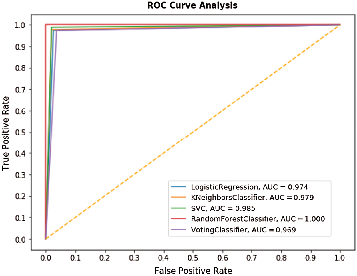
Figure 8: ROC analysis of ensemble model with different ML methods

The results attained from the experimentation reported the superior performance of ensemble model than the classical ML models in terms of precision - 94%, recall - 94%, accuracy - 94.24%, and F-score of 94%. By observing the experimental values in tables and figures, it is apparent that the ensemble model is an effective tool for GDM prediction and classification.

4  Conclusion

This research article presented an ensemble of ML-based GDM prediction and classification models. The presented model involved three processes namely, preprocessing, classification, and ensemble voting process. The input medical data was initially preprocessed in four levels such as format conversion, class labeling, normalization, and missing value replacement. Then, the preprocessed data was fed into ML model to determine the appropriate class label. At last, the ensemble model was applied to determine the appropriate class labels for the applied data instances along with the utilization of voting classifier. To validate the proficiency of the presented models, the authors conducted widespread experimentations on different aspects. From the results of experimental analysis, it is reported that the ensemble model outperformed the classical ML models and it achieved a precision of 94%, recall of 94%, accuracy of 94.24%, and F-score of 94%. In future, the predictive outcome of the presented models can be enhanced by using Deep Learning (DL) models.

Funding Statement: The authors received no specific funding for this study.

Conflicts of Interest: The authors declare that they have no conflicts of interest to report regarding the present study.

References

 1.  X. Mao, X. Chen, C. Chen, H. Zhang and K. P. Law, “Metabolomics in gestational diabetes,” Clinica Chimica Acta, vol. 475, pp. 116–127, 2017. [Google Scholar]

 2.  M. L. Geurtsen, E. E. L. V. Soest, E. Voerman, E. A. P. Steegers, V. W. V. Jaddoe et al., “High maternal early pregnancy blood glucose levels are associated with altered fetal growth and increased risk of adverse birth outcomes,” Diabetologia, vol. 62, no. 10, pp. 1880–1890, 2019. [Google Scholar]

 3.  C. E. Powe, “Early pregnancy biochemical predictors of gestational diabetes mellitus,” Current Diabetes Reports, vol. 17, no. 2, pp. 1–10, 2017. [Google Scholar]

 4.  S. Shinar and H. Berger, “Early diabetes screening in pregnancy,” International Journal of Gynecology & Obstetrics, vol. 142, no. 1, pp. 1–8, 2018. [Google Scholar]

 5.  D. D. Miller and E. W. Brown, “Artificial intelligence in medical practice: the question to the answer?,” American Journal of Medicine, vol. 131, no. 2, pp. 129–133, 2018. [Google Scholar]

 6.  Y. Xiong, L. Lin, Y. Chen, S. Salerno, Y. Li et al., “Prediction of gestational diabetes mellitus in the first 19 weeks of pregnancy using machine learning techniques,” Journal of Maternal-Fetal & Neonatal Medicine, vol. 33, no. 1, pp. 1–8, 2020. [Google Scholar]

 7.  T. Zheng, W. Ye, X. Wang, X. Li, J. Zhang et al., “A simple model to predict risk of gestational diabetes mellitus from 8 to 20 weeks of gestation in chinese women,” BMC Pregnancy and Childbirth, vol. 19, no. 1, pp. 1–10, 2019. [Google Scholar]

 8.  J. Shen, J. Chen, Z. Zheng, J. Zheng, Z. Liu et al., “An innovative artificial intelligence-based app for the diagnosis of gestational diabetes mellitus (GDM-AIdevelopment study,” Journal of Medical Internet Research, vol. 22, no. 9, pp. e21573, 2020. [Google Scholar]

 9.  I. Gnanadass, “Prediction of gestational diabetes by machine learning algorithms,” IEEE Potentials, vol. 39, no. 6, pp. 32–37, pp. 1–1, 2020. [Google Scholar]

10. Y. Srivastava, P. Khanna and S. Kumar, “February. estimation of gestational diabetes mellitus using azure AI services,” in 2019 Amity Int. Conf. on Artificial Intelligence (AICAI) IEEE, Dubai, United Arab Emirates, pp. 323–326, 2019. [Google Scholar]

11. H. Qiu, H. Y. Yu, L. Y. Wang, Q. Yao, S. N. Wu et al., “Electronic health record driven prediction for gestational diabetes mellitus in early pregnancy,” Scientific Reports, vol. 7, no. 1, pp. 1–13, 2017. [Google Scholar]

12. M. W. Moreira, J. J. Rodrigues, N. Kumar, J. A. Muhtadi and V. Korotaev, “Evolutionary radial basis function network for gestational diabetes data analytics,” Journal of Computational Science, vol. 27, pp. 410–417, 2018. [Google Scholar]

13. Y. Ye, Y. Xiong, Q. Zhou, J. Wu, X. Li et al., “Comparison of machine learning methods and conventional logistic regressions for predicting gestational diabetes using routine clinical data: a retrospective cohort study,” Journal of Diabetes Research, vol. 2020, pp. 1–10, 2020. [Google Scholar]

14. F. Du, W. Zhong, W. Wu, D. Peng, T. Xu et al., “Prediction of pregnancy diabetes based on machine learning,” in BIBE 2019; The Third Int. Conf. on Biological Information and Biomedical Engineering, Hangzhou, China, pp. 1–6, 2019. [Google Scholar]

15. G. Antonogeorgos, D. B. Panagiotakos, K. N. Priftis and A. Tzonou, “Logistic regression and linear discriminant analyses in evaluating factors associated with asthma prevalence among 10-to 12-years-old children: divergence and similarity of the two statistical methods,” International Journal of Pediatrics, vol. 2009, pp. 1–6, 2009. [Google Scholar]

16. C. Li, S. Zhang, H. Zhang, L. Pang, K. Lam et al., “Using the K-nearest neighbor algorithm for the classification of lymph node metastasis in gastric cancer,” Computational and Mathematical Methods in Medicine, vol. 2012, pp. 1–11, 2012. [Google Scholar]

17. Q. Wang, “A hybrid sampling SVM approach to imbalanced data classification,” Abstract and Applied Analysis, vol. 2014, pp. 1–7, 2014. [Google Scholar]

18. A. A. Akinyelu and A. O. Adewumi, “Classification of phishing email using random forest machine learning technique,” Journal of Applied Mathematics, vol. 2014, pp. 1–6, 2014. [Google Scholar]

19. G. Żabiński, J. Gramacki, A. Gramacki, E. M. Jakubowska, T. Birch et al., “Multiclassifier majority voting analyses in provenance studies on iron artifacts,” Journal of Archaeological Science, vol. 113, pp. 1–15, 2020. [Google Scholar]

This work is licensed under a Creative Commons Attribution 4.0 International License, which permits unrestricted use, distribution, and reproduction in any medium, provided the original work is properly cited.