Computer Systems Science & Engineering DOI:10.32604/csse.2021.016911
Article

Short-term Wind Speed Prediction with a Two-layer Attention-based LSTM

Jingcheng Qian1, Mingfang Zhu1, Yingnan Zhao2,* and Xiangjian He3

1Wujiang Power Supply Company, Suzhou, 320500, China
2School of Computer & Software, Nanjing University of Information Science & Technology, Nanjing, 210044, China
3School of Computing and Communications, University of Technology, Sydney, Australia
*Corresponding Author: Yingnan Zhao. Email: zh_yingnan@126.com
Received: 15 January 2021; Accepted: 08 March 2021

Abstract: Wind speed prediction is of great importance because it affects the efficiency and stability of power systems with a high proportion of wind power. Temporal-spatial wind speed features contain rich information; however, their use to predict wind speed remains one of the most challenging and less studied areas. This paper investigates the problem of predicting wind speeds for multiple sites using temporal and spatial features and proposes a novel two-layer attention-based long short-term memory (LSTM), termed 2Attn-LSTM, a unified framework of encoder and decoder mechanisms to handle temporal-spatial wind speed data. To eliminate the unevenness of the original wind speed, we initially decompose the preprocessing data into IMF components by variational mode decomposition (VMD). Then, it encodes the spatial features of IMF components at the bottom of the model and decodes the temporal features to obtain each component's predicted value on the second layer. Finally, we obtain the ultimate prediction value after denormalization and superposition. We have performed extensive experiments for short-term predictions on real-world data, demonstrating that 2Attn-LSTM outperforms the four baseline methods. It is worth pointing out that the presented 2Atts-LSTM is a general model suitable for other spatial-temporal features.

Keywords: Wind speed prediction; temporal-spatial features; VMD; LSTM; attention mechanism

1  Introduction

Due to its cleanliness, low cost, and sustainability, wind energy has become the mainstream new energy source. According to the latest data released by the Global Wind Energy Council (GWEC), the world's installed wind power capacity reached 651 GW in 2019 [1]. However, it poses significant challenges to the power system's operation control with a high proportion of wind power because of the randomness, volatility, and intermittency of wind farms [2]. Accurate wind speed prediction is the basis of operation control [3]. Wind speed forecasts can be divided into short-term (minutes, hours, days), medium-term (weeks, months), and long-term (years) forecasts according to different time intervals. Among them, short-term forecasting is essential for the power system to make daily dispatch plans. It has a significant impact on the economical and reliable operation of the power system.

Wind speed prediction techniques fall into the following three categories: physical, statistical, and artificial intelligence models. Physical modeling methods [4–6] mainly predict wind speed by establishing formulas between wind speed and air pressure, air density, and air humidity. The modeling process involves a large amount of calculation. Due to the complexity of wind speed and regional differences, it is challenging to establish high-precision short-term forecasts for different regions using physical models. Therefore, they are usually applied for long-term wind speed prediction in specific areas. Compared with physical models, statistical models are simple, easy, and better, so they are widely adopted in short-term wind speed prediction. Statistical models use historical wind speed data to establish a linear mapping relationship between system input and output to make predictions, for example, the kriging interpolation method [7] and the von Mises distribution [8]. There are still some commonly used methods, such as autoregressive (AR) [9] and autoregressive moving average (ARMA) [10].

Machine learning technologies are the basis of artificial intelligence models. They describe the complicated nonlinear relationship between system input and output based on a large amount of wind speed temporal data. For example, [11] used the least squares support vector machine to predict wind speed. With the vigorous development of machine learning technology, technologies in this field have been rapidly applied to short-term wind speed prediction, such as CNN, RNN, GRU, LSTM, etc. Combining the existing wind speed prediction technology and the hybrid neural network model has obtained a promising prediction result [12–14]. However, the current short-term wind speed prediction models only focus on time series data, and the wind speed data of the sites near the target wind farm also contain rich information. Data analysis based on spatial-temporal correlation has become a research hot spot [15,16]. In addition to temporal data, geographic spatial relationships are also considered to improve prediction accuracy. Moreover, the attention mechanism (AM) has recently become a research hot spot [17,18]. It builds an attention matrix to enable deep neural networks to focus on crucial features during training to avoid the impact of insensitive features.

In this paper, we introduce two-layer attention-based LSTM (2Atts-LSTM) networks. Experiments on real-world data show that they are superior to other baselines.

The main contributions of this article can be summarized as follows:

(1) 2Atts-LSTM, a novel deep architecture for short-term wind speed prediction, is proposed, which integrates the attention mechanism and LSTM into a unified framework. This model achieves spatial feature and temporal dependency extraction automatically.

(2) VMD technology is combined with 2Attn-LSTM to obtain a relatively stable subsequence. It can eliminate the uncertainty of the actual wind speed.

The rest of the paper is organized as follows: Section 2 gives relevant background theories, including VMD and LSTM networks; Section 3 illustrates the algorithm proposed in the article; Section 4 presents the experimental results, compared with the baselines; Section 5 concludes this paper and provides further work.

2  Background Theories

2.1 VMD

Based on empirical mode decomposition (EMD), the variational mode decomposition (VMD) proposed by Dragomirestskiy et al. [19] is a new type of complicated signal decomposition method. It decomposes the signal into limited bandwidths with different center frequencies according to the preset number of modes.

Using VMD, the original wind speed sequence with strong nonlinearity and randomness can be decomposed into a series of stable mode components. Fig. 1 shows the flowchart of the VMD algorithm. Suppose the wind speed data after preprocessing are X~(t)l . The process is as follows:

(1) Assuming that each mode has a limited bandwidth with a center frequency, we now look for modes so that the sum of each mode's estimated bandwidth is the lowest, expressed as

min|uk|.|ωk|⁡{∑k=1K‖∂t[(δ(t)+jπt)∗uk(t)l]e−jwkt‖22s.t.∑k=1Kuk(t)l=X~(t)l (1)

(2) Solving the above model, introduce the penalty factor α and Lagrangian penalty operator λ(t) , transform the constraint problem into the nonconstraint problem, and obtain the augmented Lagrangian expression.

L({uk},{ωk},λ)=α∑K‖∂t[(δ(t)+jπt)∗uk(t)]∙e−jwkt‖22+‖f(t)−∑Kuk(t)‖22+⟨λ(t)f(t)−∑Kuk(t)⟩ (2)

(3) Update parameters uk , ωk and λk iteratively by the alternating direction method of multipliers, which is defined as

u^kn+1=f^(ω)−∑i≠ku^i(ω)+λ^(ω)21+2α(ω−ωk)2 (3)

ωkn+1=∫0∞ω|u^kn+1(ω)|2dω∫0∞|u^kn+1(ω)|2dω (4)

where f^(ω) , u^i(ω) , λ^(ω) and u^kn+1(ω) represent the Fourier transforms of f(ω) , ui(ω) , λ(ω) and ukn+1(ω) , and n is the number of iterations.

(4) For a given precision e > 0, if  ∑i‖u^ kn+1−u^ kn‖22‖u^ kn‖22<e , then stop the iteration. Otherwise, return to

(5) Finally, we can get K decomposed Fkt,l .

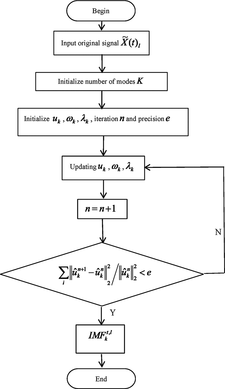
Figure 1: The flowchart of VMD algorithm

Fig. 2 shows the wind speed subsequences, IMF, with different frequencies but stronger regularity by VMD.

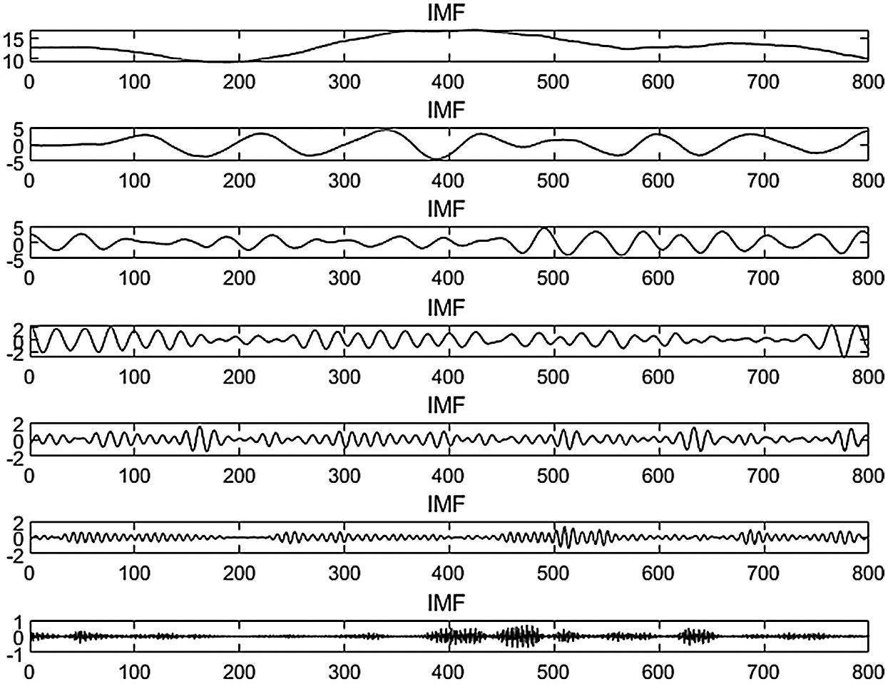
Figure 2: Wind speed is decomposed by VMD

2.2 LSTM

LSTM [20], a variant of the recurrent neural network (RNN), shows superior performance in processing sequential data. It overcomes the problem of “long-term dependencies” [21]. Due to its tremendous learning capacity, LSTM has been widely used in various kinds of tasks, such as speech recognition [22], software-defined network (SDN) [23], and some prediction cases, i.e., trajectory [24], oil price [25], and even the number of confirmed COVID-19 cases [26]. In the usual applications, the stacked LSTM network is the most basic and simplest structure with high performance. In this paper, the proposed 2Attn-LSTM falls into this category.

Each LSTM cell unit consists of an internal memory cell ct and three gates, i.e., forget gate ft , input gate it , and output gate ot . ht is the final state determined by ct and ot . The memory cell will store the previous data for a long time controlled by the input and output gates. At the same time, the information stored in the memory cell can be cleared by the forget gate. The formulations in the LSTM are given by Eqs. (5)–(9).

it=sigmoid(Whiht−1+WxiFkt,l+bi) (5)

ft=sigmoid(Whfht−1+WxfFkt,l+bf) (6)

ot=sigmoid(Whoht−1+WhxFkt,l+wcoct) (7)

ct=ft⊗ct−1+it⊗(tanh⁡(Whcht−1+WxcFkt,l+bc)) (8)

ht=ot⊗tanh⁡(ct) (9)

where whi , wxi , bi , whf , wxf , bf , whc , wxc , bc , who , whx , wco are learnable parameters of input gate, forget gate, memory cell, output gate and final state, respectively.

3  Methodology

The proposed 2Attn-LSTM method, illustrated in Fig. 3, consists of data preprocessing, decomposition of VMD, LSTM encoder with Attention1 and LSTM decoder with Attention2. Then, it gets each IMF’s prediction value. After denormalization and superposition, we can obtain the final wind speed prediction. The preprocessing stage contains data cleaning and normalization. Then, it decomposes the preprocessed data into components, Fkt,l , by VMD. The model training phase contains an encoder and decoder; that is, the first layer handles the spatial features, and the second layer manages the temporal features. Here, we adopt an attention mechanism into the architecture, which has been widely applied recently.

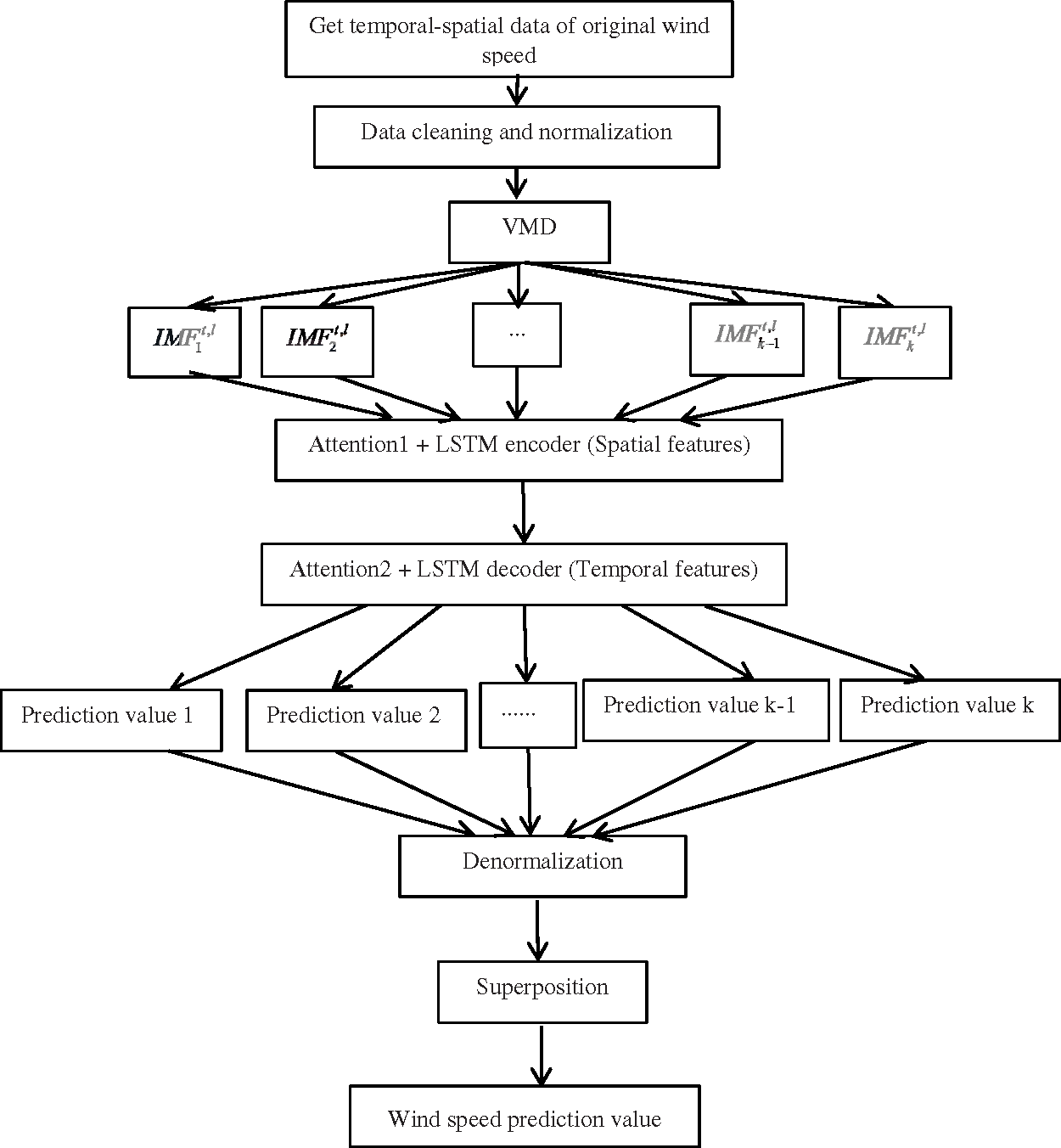
Figure 3: Framework of the presented approach

3.1 Data Processing

Obtain the original space-time wind speed sequence of the target site X(t)l . For missing data, repeated data, and jump data, replace with the average wind speed near the value. After normalization, we obtain X~(t)l , where t∈RT , l∈RL , T is the time lag, and L is the number of neighboring sites of the target site. The normalization formula is

X~(t)l=X(t)l−Xmin(t)lXmax(t)l−Xmin(t)l (10)

where Xmax(t)l is the maximum temporal wind speed of site l , and Xmin(t)l is the minimum temporal wind speed of site l . X(t)l is the value before normalization, and X~(t)l is the value after normalization of site l .

After the handling of the 2-layer LSTM network, we need denormalization and superposition. The denormalization formula is given as follows:

Y(t)l=Y~(t)l(IMFmax(t)l−IMFmin(t)l)+IMFmin(t)l (11)

where IMFmax(t)l and IMFmin(t)l are the maximum and minimum IMF components of site l , respectively. Y~(t)l is the normalization value, and Y(t)l is the denormalized result.

3.2 Temporal-Spatial Feature Model

In the proposed 2Attn-LSTM framework, we process the temporal-spatial data. Except for the general sequential features, the spatial data do have plenty of information helpful for wind speed prediction. Zhu et al. [15] proposed a deep architecture, termed PSTN, integrating CNN and LSTM, to learn temporal and spatial correlations jointly for short-term wind speed prediction.

However, Zhu et al. [15] embedded the temporal-spatial features into a 2D matrix, named SWSM. The item in SWSM is defined by x(i,j)t∈RM×N , where M×N is the spatial square of the target site. Instead of SWSM, we specify one IMF time series as the target series for making predictions, while other IMF series are used as features. Furthermore, we separated the spatiotemporal features into spatial data, served as the input of the encoder of 2Attn-LSTM, and temporal data, served as the input of the decoder of 2Attn_LSTM. The scheme is superior to PSTN in both space requirements and time complexity. Suppose the time window length is T , the number of neighboring sites is L , and the number of IMF components is K . We use Fkt,l=(fk1,l,fk2,l,...,fkT,l)∈RT to denote the temporal features and Fkt,l=(fkt,1,fkt,2,...,fkt,L)∈RL to describe the spatial features.

As illustrated in Fig. 4, we decompose the original wind speed into K IMF components, denoted by IMFkt,l . The features along the x -direction are temporal features, i.e., IMFkt,l=(IMFk1,l,IMFk2,l,...,IMFkT,l)∈RT . The y -direction features are IMFkt,l=(IMF1t,l,IMF2t,l,...,IMFKt,l)∈RK , and they denote the K IMF components. The z -direction features are spatial features, i.e., IMFkt,l=(IMFkt,1,IMFkt,2,...,IMFkt,L)∈RL .

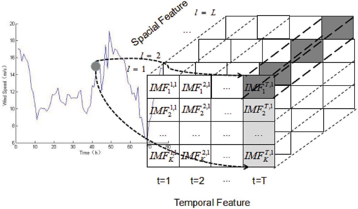
Figure 4: Model of spatial-temporal feature

3.3 Network Architecture

Fig. 5 depicts the hierarchy of 2Attn-LSTM, which follows the encoder-decoder architecture. We adopt two separate LSTMs. One is to encode the spatial features, and the other decodes the temporal features. The encoder captures the temporal correlations of IMF components at each time by referring to the previous hidden state of the encoder, previous values of sensors and the spatial information. In the decoder, we use temporal attention to adaptively select the relevant previous time intervals for making predictions.

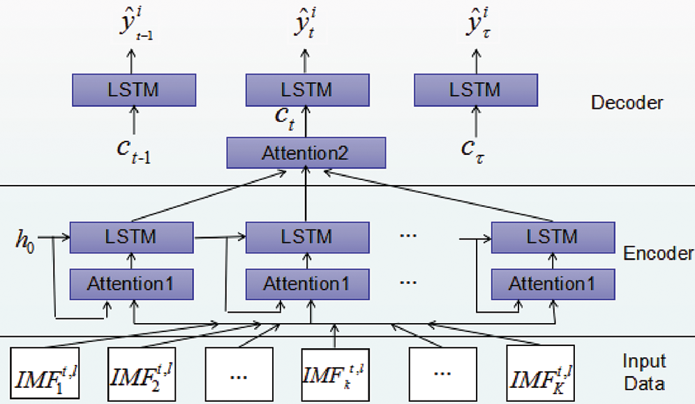
Figure 5: 2Attn-LSTM hierarchy

In the encoder part, we calculate Attention1 as follows:

atl=exp⁡((1−λ)gtl+λIi,j)∑j=1Kexp⁡((1−λ)gtj+λIi,j) (12)

where gtl is the weight attention of i and j sites, which is calculated as follows:

gtl=vgTtanh⁡(Wg[ht−1;ct−1]+UgFkt,j+Wg′Fkt,iug+bg) (13)

Here, vg , ug , bg , Wg and Ug are learnable parameters, and [;] is the connection computation. ht−1 and ct−1 are the hidden state and memory unit cell at time t−1 of the LSTM encoder, respectively. Ii,j is the mutual information of i , j sets. It is computed as follows:

Ii,j=H(Fkt,i)+H(Fkt,j)−H(Fkt,i,Fkt,j) (14)

H(Fkt,i)=−∑f∈Fkt,iPFkt,i(f)log⁡(PFkt,i(f)) (15)

H(Fkt,i,Fkt,j)=−∑f∈Fkt,i,f′∈Fkt,iPFkt,iFkt,i(f,f′)log⁡(PFkt,iFkt,i(f,f′)) (16)

where H(Fkt,i) is the entropy of Fkt,i , H(Fkt,i,Fkt,j) is the union entropy of Fkt,i and Fkt,j , and P(∙) is the probability density function.

In the encoder, the following formula is used to update the hidden state at time t :

ht=fe(ht−1,atl) (17)

where fe is the LSTM cell of the encoder, and ht−1 is the hidden state at time t−1 .

In the decoder, we use the following equation to update the hidden state at time t′ :

ht′′=fd(ht′−1′,[f^t′−1i;at′]) (18)

where fd is the LSTM cell of the decoder, and f^t′−1i is the prediction component at time t′−1 . Attention2 is calculated as follows:

ut′o=vdTtanh⁡(Wd′[ht′−1′;ct′−1′]+Wdho+bd) (19)

γt′o=exp⁡(ut′o)∑j=1Texp⁡(ut′j) (20)

a^t′=∑o=1Tγt′oho (21)

where Wd , Wd′ , vd and bd are learnable parameters. ht′−1′ and ct′−1′ are the hidden state and memory cell of the decoder in LSTM at time t′−1 , respectively.

The final prediction component is

f^t′i=vyT(Wm[at′;ht′]+bm)+by (22)

where Wm , bm , vy and by are parameters.

4  Experiments

4.1 Settings

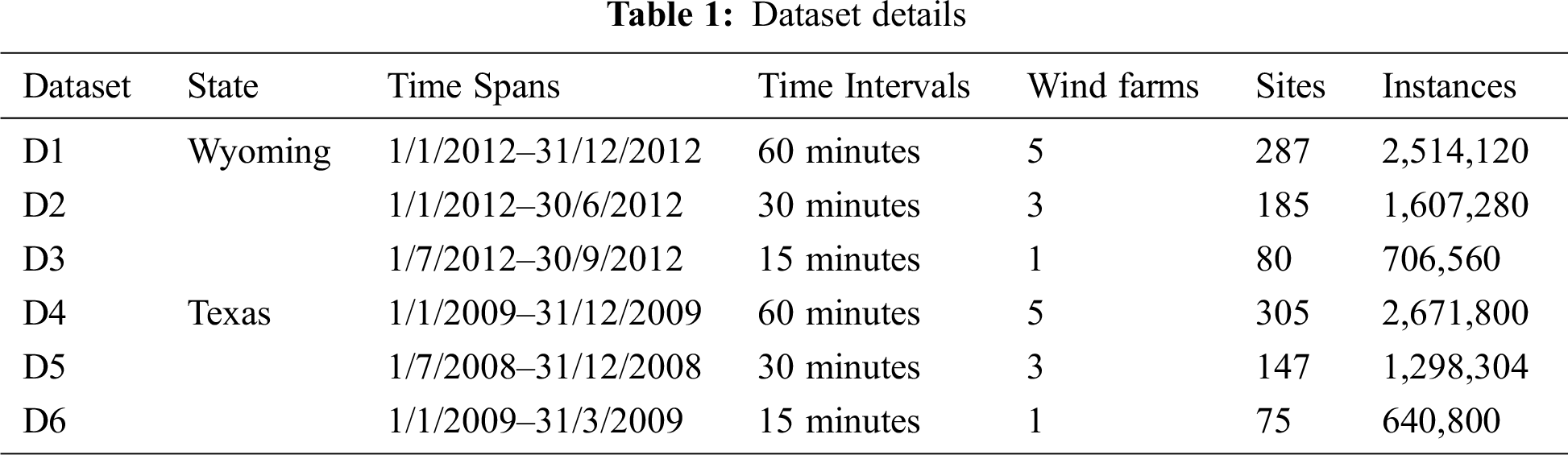
We perform our experiments over the Wind Integration National Data set (WIND), provided by the National Renewable Energy Laboratory (NREL). It contains wind speed data for more than 126,000 sites in the United States for the years 2007–2013. We consider 6 different datasets based on WIND, as depicted in Tab. 1. They belong to Wyming and Texas states. In each state, we choose 5, 3, and 1 wind farms with different time intervals (i.e., 1 hour, 30 minutes, 15 minutes) and time spans (i.e., 1 year, six months, three months) to guarantee plenty of instances. For example, 5 wind farms of 286 sites in Wyoming state are conducted in the experiment. The D1 dataset has 2,514,120 instances with a 1-hour time interval during 2012.

We use general criteria to evaluate the proposed 2Attn-LSTM model, that is, the mean absolute error (MAE) and root mean squared error (RMSE), which are widely adopted as the evaluation indices in the task of wind speed prediction. They are given by the following:

EMAE=1N∑i=1N|Yi−Y^i| (23)

ERMSE=1N∑i=1N(Yi−Y^i)2 (24)

where N is the number of predictions, and i is the sequence number of the forecast point. Yi and Y^i denote the ground truth and predicted wind speeds, respectively.

4.2 Baselines

We compare our model with 4 baselines. They are BP, ARIMA [27], LSTM and PSTN [15]. The back propagation (BP) neural network algorithm is a multilayer feedforward network trained according to the error back propagation algorithm and is one of the most widely applied neural network models. Autoregressive Integrated Moving Average (ARIMA) is actually a class of models that explains a given time series based on its own past values, that is, its own lags and the lagged forecast errors, so that equation can be used to forecast future values. It is a well-known model for forecasting future values in a time series. As a variant of RNN, LSTM shows superior performance in processing sequential data.

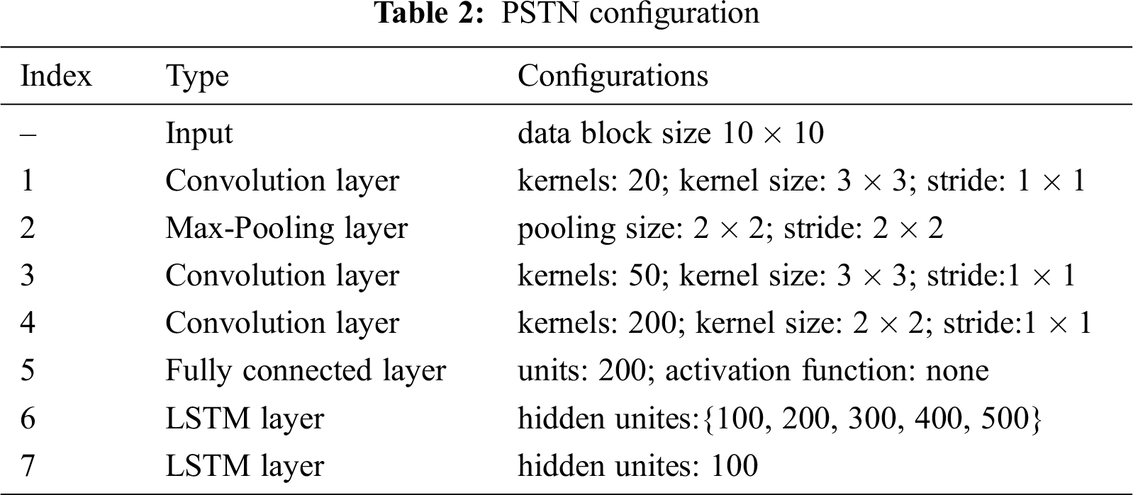
The three methods mentioned above are classical models in short-term wind speed prediction. The PSTN was recently proposed to leverage both temporal and spatial correlations. It integrates CNN and LSTM to form a unified framework. To evaluate the presented 2Attn-LSTM with PSTN, we choose the same configuration in Zhu et al. [15], as shown in Tab. 2.

4.3 Implementation Details

The determination of the optimal hyperparameters is still an open issue. Specifically, we divided the dataset into three subsets, i.e., training set, validation set and testing set at a ratio of 6:1:3. The training set serves for model training, including searching for optimal hyperparameters, and the validation set is used for model selection and overfitting prevention. We use testing data to test the model performance. All the baselines are determined in this way as well.

In the presented 2Attn-LSTM, there are many hyperparameter settings during the training phase. We set the batch size to 256 and the learning rate to 0.01. We set τ=6 to make short-term predictions. The trade-off parameter λ is empirically fixed from 0.1 to 0.5. For the length of window size T , we set T∈{6,12,24,36,48} . For simplicity, we use the same hidden dimensionality at the encoder and the decoder and conduct a grid search over {32, 64, 128, 256}. Moreover, we use stacked LSTMs (the number of layers is denoted as q ) as the units of the encoder and decoder to enhance our performance. The setting is in which q=2 , m=n=64 and λ=0.2 outperform the others in the validation set.

The TensorFlow deep learning framework based on the Python platform builds our model as well as the baselines. All the methods are carried out on a 64-bit PC with an Intel Core i5-7600 CPU/32.00 GB RAM. We test different hyperparameters to find the best setting for each.

4.4 Short-term Wind Speed Prediction

To evaluate the prediction performance of the presented model, we conduct experiments with a prediction horizon ranging from 10 minutes to 1 hour. The prediction performance of all models is evaluated on 6 testing sets by MAE and RMSE indices.

The results shown in Tab. 3 illustrate that the proposed 2Attn-LSTM model holds the dominant position over the other models, while BP produces the worst prediction results. BP performs fairly poor with longer prediction horizons. For example, BP is 3.0% lower than the ARIMA 15-minute ahead prediction, while it increases to 10% when performing the 1-hour ahead prediction in terms of MAE. Although ARIMA outperforms BP, it is still inferior to LSTM, which implies that LSTM is more efficient in capturing temporal information. This mainly benefits from the working mechanism, i.e., the gates and the memory cell update information and prevent the model from vanishing the gradient. Specifically, PSTN improves the average MAE and RMSE by 14% and 3%, respectively, compared to LSTM. Integrating spatial and temporal features in the PSTN contributes to the best performance. The proposed 2Attn-LSTM method outperformed the PSTN in MAE by 8% in the 15-min horizon and 27.5% in the 1-hour ahead prediction task. The reasons for this may lie in the following two aspects. (1) The 2Attn-LSTM model handles the VMD first, which decomposes the original wind speed sequence with strong nonlinearity, and randomness can be decomposed into a series of stable modes. It plays a more critical role when the prediction horizon increases. (2) It considers both spatial and temporal features, such as PSTN, which is helpful for prediction.

Figs. 6 and 7 show the comparison of these five methods in the Wyoming dataset by RMSE and in the Texas dataset by MAE. Fig. 6 implies that for the same method, the shorter the time interval is, the higher the prediction performance. Fig. 7 lists the comparison among 5 models by MAE. It can be concluded that 2Attn-LSTM achieves the best performance.

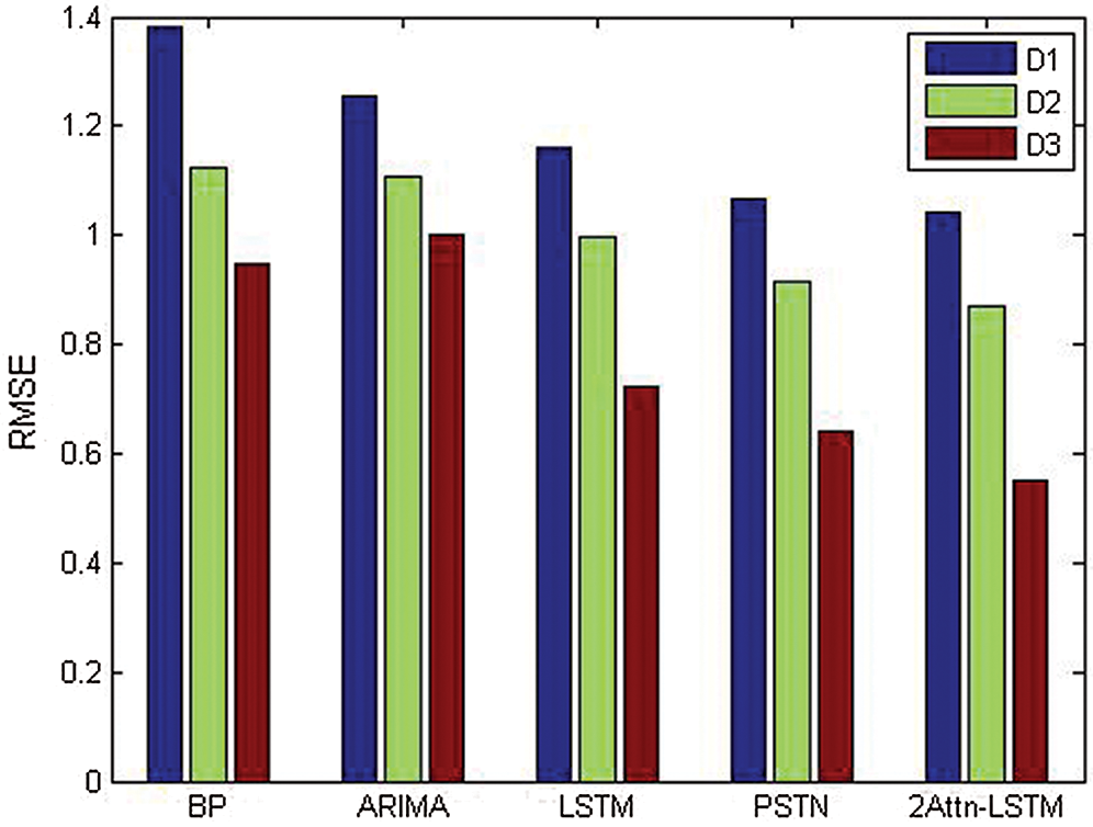
Figure 6: RMSE in the Wyoming dataset

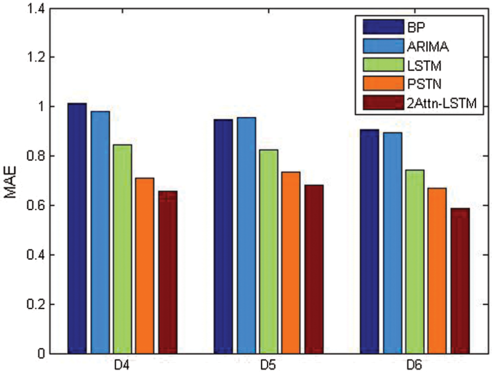
Figure 7: MAE in the Texas dataset

5  Conclusion and Future Work

We propose a deep 2Atts-LSTM architecture for short-term wind prediction, which integrates spatial-temporal features into a unified framework. In the first layer, an encoder of LSTM with mutual-information-based attention is adopted to extract the spatial features from the IMF components by VMD of wind speed. In the second layer, we employ temporal attention to select the relevant time step to make predictions adaptively. Experiments on real-world data illustrate the superior performance against 4 baselines in terms of MAE and RMSE simultaneously.

It is worth pointing out that the presented 2Atts-LSTM is a general model suitable for other spatial-temporal features. Furthermore, we will investigate how to integrate more sensor data into the model, such as atmospheric pressure and temperature. We think it is feasible to combine more variables; although, it is challenging to achieve the input selection and train the more complicated framework.

Acknowledgement: Thank you for the Wind Integration National Data set (WIND) provided by National Renewable Energy Laboratory (NREL).

Funding Statement: This work is supported in part by the Priority Academic Program Development of Jiangsu Higher Education Institutions, Natural Science Foundation of China (No. 61103141, No. 61105007 and No. 51405241) and NARI Nanjing Control System Ltd. (No. 524608190024).

Conflicts of Interest: The authors declare that they have no conflicts of interest to report regarding the present study.

This work is licensed under a Creative Commons Attribution 4.0 International License, which permits unrestricted use, distribution, and reproduction in any medium, provided the original work is properly cited.