Inverse Length Biased Maxwell Distribution: Statistical Inference with an Application

Amer Al-Omari; Ayed Alanzi

doi:10.32604/csse.2021.017362

[BACK]

Computer Systems Science & Engineering DOI:10.32604/csse.2021.017362
Article

Inverse Length Biased Maxwell Distribution: Statistical Inference with an Application

Amer Ibrahim Al-Omari1 and Ayed R.A. Alanzi2,*

1Department of Mathematics, Faculty of Science, Al al-Bayt University, Mafraq, Jordan
2Department of Mathematics, College of Science and Human Studies at Hotat Sudair, Majmaah University, Majmaah 11952, Saudi Arabia
*Corresponding Author: Ayed R. A. Alanzi. Email: a.alanzi@mu.edu.sa
Received: 28 January 2021; Accepted: 14 March 2021

Abstract: In this paper, we suggested and studied the inverse length biased Maxell distribution (ILBMD) as a new continuous distribution of one parameter. The ILBMD is obtained by considering the inverse transformation technique of the Maxwell length biased distribution. Statistical characteristics of the ILBMD such as the moments, moment generating function, mode, quantile function, the coefficient of variation, coefficient of skewness, Moors and Bowley measures of kurtosis and skewness , stochastic ordering, stress-strength reliability, and mean deviations are obtained. In addition, the Bonferroni and Lorenz curves, Gini index, the reliability function, the hazard rate function, the reverse hazard rate function, the odds function, and the distributions of order statistics for the ILBMD, are presented. The ILBMD parameter is estimated using the maximum likelihood method, the method of moments, the maximum product of spacing technique, the ordinary and weight least square procedures, and the Cramer-Von-Mises methods. The Fishers information, as well as the Rényi and q-entropies, are derived. To investigate the usefulness of the proposed lifetime distribution and to illustrate the purpose of the study, a real dataset of the relief times of 20 patients receiving an analgesic is used.

Keywords: Maxell distribution; inverse length biased Maxwell distribution; Fisher’s information; methods of estimation; goodness of fit tests

1 Introduction

A random variable W follows a Maxwell distribution with scale parameter $α$ $α$ , if its probability density function (pdf) and cumulative distribution function (cdf), respectively, are given by

$fMD(w;α)=2πw2α3e−w22α2,0<w<∞,α>0,$ (1)

$FMD(w;α)=Erf(wα2)wα2πe−w22α2,$ (2)

where $Erf(z)=2π∫0ze−t2dt$ . In the literature of the probability distributions, uni-modal and skewed to the right characteristics are very important to the distribution of interest. One of these distributions is the Maxwell distribution, which is a well-known lifetime distribution in physics and statistical mechanics. Reference Iriarte et al. [1] suggested a gamma-Maxwell distribution. The tail behavior of the generalized Maxwell distribution is considered by Huang et al. [2]. Recently, Saghir et al. [3] suggested a length-biased Maxwell distribution (LBMD) as a modification of the base Maxwell distribution based on the weighted distribution suggested by Rao et al. [4], to obtain the probability density function given by:

$fLBMD(w;α)=w32α4e−w22α2,0<w<∞,α>0,$ (3)

and a cumulative distribution function defined as

$FLBMD(w;α)=1−(w22α2+1)e−w22α2,0<w<∞,α>0.$ (4)

The mode and median of the LBMD are $wM=α3$ and $E(W)=3α42π$ , respectively. For more information about the LBMD see [3]. Due to the large number of data in these times, a large number of distributions are suggested based several philosophies, assuming that the suggested distributions are more flexible in modeling data. For example, [5] introduced Marshall–Olkin length-biased Maxwell distribution. Reference Singh et al. [6] suggested length-biased weighted Maxwell distribution and [7] considered estimation of the inverse Maxwell distribution parameter. Reference Garaibah et al. [8] suggested size-biased Ishita distribution and [9] introduced transmuted Ishita distribution. The Marshall-Olkin length-biased exponential distribution is proposed by Shraa et al. [10]. A new mixture continuous Darna distribution is suggested by Al-Omari et al. [11,12] proposed length-biased Suja distribution. Reference Sharma et al. [13] studied the power size biased two-parameter Akash distribution with some statistical properties and real data applications. Reference Al-Omar et al. [14] proposed length and area biased Maxwell distributions. Reference Gharaibeh [15] suggested Top-Leone Mukherjee-Islam distribution and [16] proposed transmuted Aradhana distribution.

The rest of this paper is organized as follows: In Section 2, we present the derivation of the suggested distribution. Section 3 deals with the main statistical properties of the ILBMD. Different methods of estimation for the distribution parameter are given in Section 4. In Section 5, a simulation study is conducted to investigate the distribution. An application of real data is presented in Section 6 and the paper is concluded in Section 7.

2 Derivation of the Suggested Model

If a random variable W has a LBMD with pdf given in (3), then the random variable $X=1W$ is said to follow the inverse LBMD. The pdf and cdf of the inverse length-biased Maxwell distribution (ILBMD), respectively are given by

$fILBMD(x;α)=12α4x5e−12α2x2,0<x<∞,α>0,$ (5)

and

$FILBMD(x;α)=(1+12α2x2)e−12α2x2,0<x<∞,α>0.$ (6)

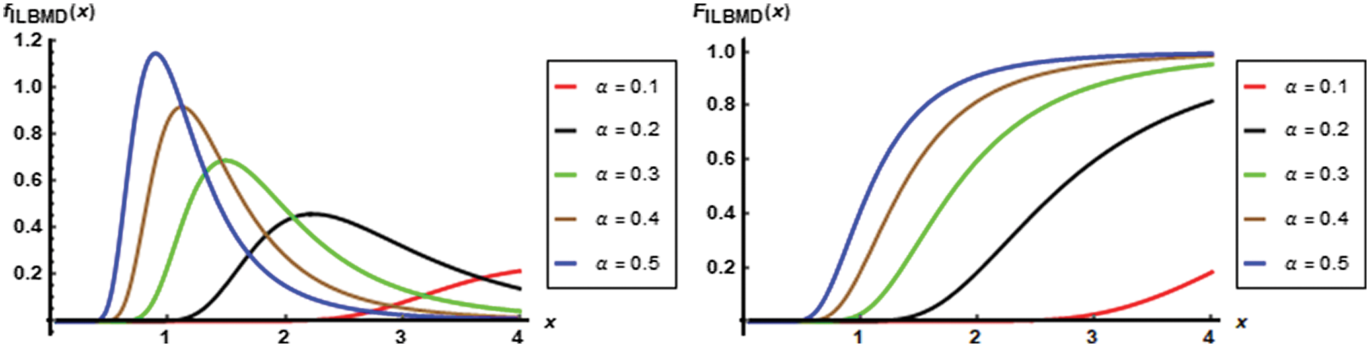
Plots of the pdf and cdf of the ILBMD are presented in Fig. 1 for various distribution parameter. Fig. 1, revealed that the pdf of the suggested distribution is skewed to the right and be more flatting as $α$ values are increasing. Also, the pdf of the ILBMD can exhibit various behavior depending on the values of the parameter.

images

Figure 1: The ILBMD pdf and cdf plots for $α=0.1,0.2,0.3,0.4,0.5$

3 Statistical Properties

In this section, the main properties if the proposed model are presented.

3.1 Reliability Analysis

The reliability is a well-known in engineering where it gives the probability for surviving at least time t of a product operate, while the hazard function shows the nature of failure rate related to the product. Generally, the reliability and hazard functions are fundamental to study the characteristics of the time to event data. Figs. 2 and 3 are the plots of the hazard, reliability reversed hazard, and the odds functions of the ILBMD for $α=0.1,0.2,0.3,0.4,0.5$ .

• Hazard rate function: The hazard rate (HR) function is a very important property in characterizing any lifetime distribution. The HR of the ILBMD is given by

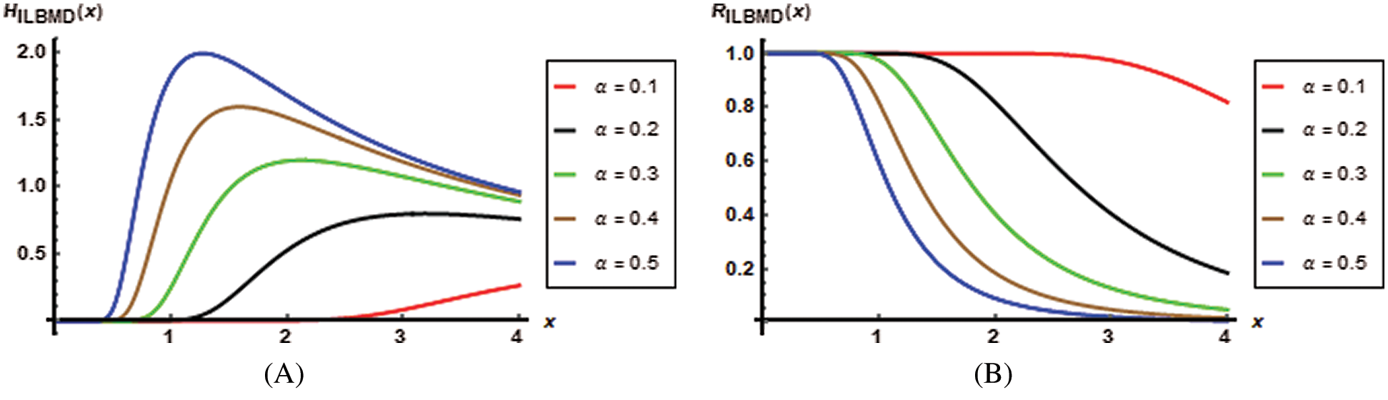
$HILBMD(x;α)=fILBMD(x;α)1−FILBMD(x;α)=12α4x5e−12α2x21−(1+12α2x2)e−12α2x2.$ (7)

images

Figure 2: The hazard (A) and reliability (B) functions of the ILBMD plots for $α=0.1,0.2,0.3,0.4,0.5$

images

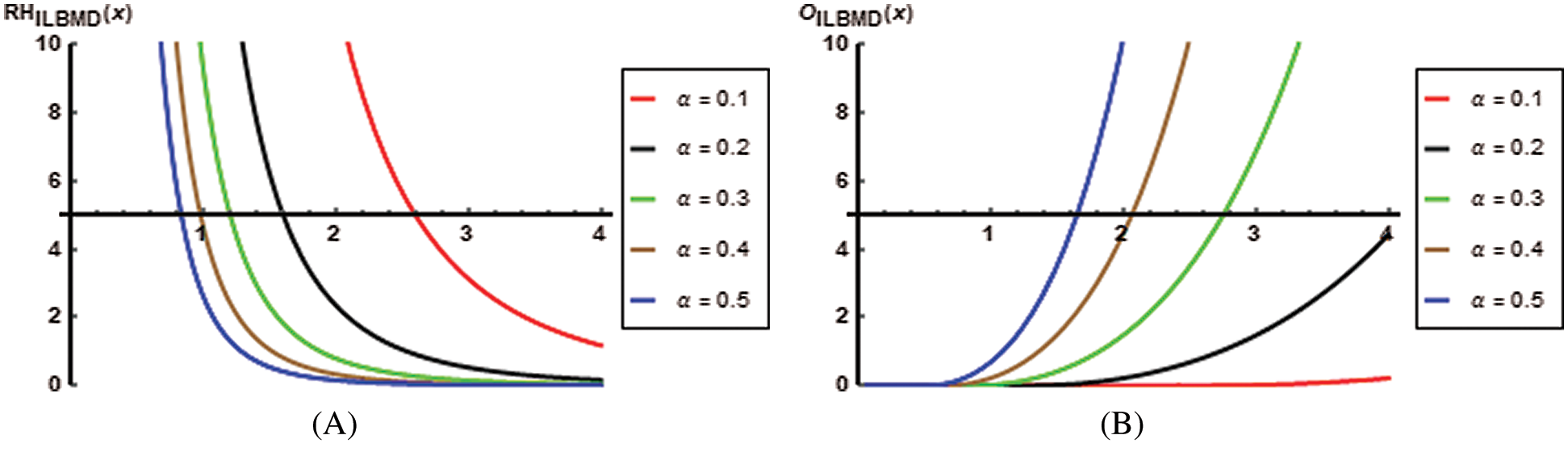
Figure 3: The reverse hazard (A) and odds (B) functions of the ILBMD plots for $α=0.1,0.2,0.3,0.4,0.5$

To determine the shape of the HR function we followed the technique of [17] which is defined as $Φ(x;α)=−f/(x;α)f(x;α)$ which only depends on the pdf of the distribution. He proved that if $Φ/(x)>0$ for all $x∈(0,x0)$ , while $Φ/(x0)=0$ , and $Φ/(x)<0$ for all $x∈(x0,∞)$ , the distribution has upside down bathtub hazard rate (UBT). For the ILBMD we have $Φ(x;α)=5x−1x3α2$ and $Φ/(x;α)=3α2x4−5x2$ . Now, it is found that $Φ(3/5α;α)=0$ , that is $x0=3/5α$ , and hence for the ILBMD we have that $Φ(x;α)$ is increasing on the interval $(0,3/5α)$ and it is decreasing on the interval $(3/5α,∞)$ as illustrated in Fig. 2A. Therefore, the proposed ILBMD is useful in reliability data and medical fields due its skewness to the right with UBT shape of hazard rate function.

• Reliability function: The reliability function of the ILBMD distribution is

$RILBMD(x;α)=1−FILBMD(x;α)=1−(1+12α2x2)e−12α2x2$ (8)

Fig. 2B shows that the reliability plots of the ILBMD intersect at the point $f(x)=1$ for $x=0$ , while as x goes to infinity, the reliability function decreases and goes to zero.

• Reversed hazard function: The reversed hazard function of the ILBMD is defined as

$RHILBMD(x;α)=fILBMD(x;α)FILBMD(x;α)=12α2x2+1$ (9)

• Odds function: The odds function of the ILBMD is given by

$OILBMD(x;α)=FILBMD(x;α)1−FILBMD(x;α)=2α2x2+12α2x2e12α2x2−2α2x2−1.$ (10)

Based on Fig. 3 it can be noted that the reversed hazard decreases with negative J-shaped distribution, while the odds function increases taking the J-shaped with more flatting for small amounts of the parameter $α$ .

3.2 The Mode

In this section, the mode of the ILBMD is derived. Since the pdf $fILBMD(x;α)$ of the model and its logarithm are maximized at the same point, then for simple calculation, take the derivative of the logarithm of the function $fILBMD(x;α)$ as

$Υ=ln⁡fILBMD(x;α)=−ln⁡(2α4x5)−12α21x2.$

The derivative of $Υ$ with respect to x yields $∂Υ∂x=−5x+12α22x3.$ Equating the preceding derivative to 0 leads to $−5x+12α22x3=0$ and $xMode=±15α.$ But since $α>0$ , then the mode of the ILBMD is $xMode=15α.$ It is clear that the distribution is a unimodal and the mode decreases with increases values of α.

3.3 Moments and Quantile Function

In this section, we derived the various moments of the suggested ILBMD as

• Let $X∼fILBMD(x;α)$ , then the rth moment of X is

$E(XILBMDr)=Γ(2−r2)2r2αr,α>0,r=1,2,3,...$ (11)

• If $X∼fILBMD(x;α)$ , then the moment generating function of X is

$MILBMD(t)=t4log⁡[e]4MeijerG[{{},{}},{{−2,−32,0},{}},t2log⁡[e]28α2]64πα4,α>0,$ (12)

where $MeijerG((a1…anan+1…ap),(b1…bmbm+1…bq),z)$ is the Meijer G function $Gpqmn(z|a1…apb1…bq)$ .

From Eq. (11), the first and second moments of the ILBMD, respectively, are given as

$E(XILBMD1)=12απ2$ and $E(XILBMD2)=12α2$ .

• The variance of the ILBMD is

$Var(XILBMD)=E(XILBMD2)−(E(XILBMD1))2=12α2−(12απ2)2=4−π8α2.$ (13)

• The degree of long-tail is measured by skewness (Sk) and for the ILBMD it is given by

$SkILBMD=2(π−2)π(−1π−4)3/2=5.08834.$ (14)

• The coefficient of variation of the ILBMD is

$CvILBMD=22π12α2−π8α2α4(α2)3/2=4π−1=0.522723,$ (15)

which is a very small value.

• Let $X∼fILBMD(x;α)$ , then the rth order inverse moment about the origin of X is

$E(1XILBMDr)=2r2αrΓ(2+r2),r=1,2,3,...$ (16)

Based on Eq. (6), the harmonic mean of the ILBMD distribution can be obtained for $r=1$ as given by

$E(1XILBMD)=32π2α.$ (17)

If $Q(k)$ is the quantile function of order k of the ILBM random variable, then it can be the solution of the equation

$ln⁡k+12α2Q2(k)=ln⁡(1+12α2Q2(k)).$ (18)

The Moors and Bowley measures of kurtosis and skewness, respectively, are given by

$Mk=Q(78)−Q(58)+Q(38)−Q(18)Q(68)−Q(28)andBsk=Q(34)−2Q(12)+Q(14)Q(34)−Q(14).$ (19)

3.4 Fishers Information

Theorem: Let $X∼fILBMD(x;α)$ , then the Fisher’s information of $α$ is $FIILBMD(α)=8α2.$

Proof: To find the Fisher’s information of the ILBMD, we have

$ln⁡fILBMD(x;α)=−5log⁡[x]+log⁡[12α4]−12α2x2.$

The first derivative of this function with respect to $α$ yields

$∂ln⁡fILBMD(x;α)∂α=2e12x2α2x5(e−12x2α22x7α7−2e−12x2α2x5α5)α4.$

Again differentiate the last equation with respect to $α$ to get

$∂2ln⁡fILBMD(x;α)∂α2=8α3x5e12α2x2(e−12α2x22α7x7−2e−12α2x2α5x5)−2αx3e12α2x2(e−12α2x22α7x7−2e−12α2x2α5x5)+2e12x2α2x5(e−12x2α22x9α10−11e−12x2α22x7α8+10e−12x2α2x5α6)α4.$

Now, take the expectation of $∂2ln⁡fILBMD(x;α)∂α2$ as

$−E(∂2ln⁡fILBMD(x;α)∂α2)=−∫0∞∂2ln⁡fILBMD(x;α)∂α212α4x5e−12α2x2dx=8α2.$

This information is very helpful in determining the variance of estimator or lower bound of an estimator.

3.5 Order Statistics

Let $X(1:n),X(2:n),...,X(n:n)$ be the order statistics of the random sample $X1,X2,...,Xn$ selected from a pdf and cdf $fILBMD(x;α)$ and $FILBMD(x;α)$ , respectively. The pdf of the ith order statistics say $X(i:n)$ , is

$f(i:n)(x)=n!(i−1)!(n−i)![F(x)]i−1[1−F(x)]n−if(x)=n!(i−1)!(n−i)!∑k=0n−i(−1)k(n−ik)12α4x5(1+12α2x2)k+i−1(e−12α2x2)k+i,$ (20)

and the corresponding cdf is defined as

$F(i:n)(x)=∑j=tn(nj)F(x)]j[1−F(x)]n−j=∑j=tn∑k=0n−i(−1)k(nj)(n−ik)[(1+12α2x2)e−12α2x2]j+k.$ (21)

3.6 Stochastic Ordering

The stochastic ordering can be considered to compare the behavior of two random variables. Let X and Y be two random variables, then X is said to be smaller than in

1) Mean residual life order $(X≤mrl⁡Y)$ if $mX(x)≤mY(x)$ for all x;

2) Likelihood ratio order $(X≤lr⁡Y)$ if $fX(x)fY(x)$ decreases in x;

3) Hazard rate order $(X≤hr⁡Y)$ if $hX(x)≥hY(x)$ for all x;

4) Stochastic order $(X≤st⁡Y)$ if $FX(x)≥FY(x)$ for all x.

Based on these relations, we have $(X≤lr⁡Y)⇒(X≤hr⁡Y)⇓(X≤st⁡Y)⇒(X≤mrl⁡Y)$ .

Theorem 2: Let $XILBMD∼fX(x;α)$ and $YILBMD∼fY(x;θ)$ . If $θ<α$ , then $(X≤lr⁡Y)$ , and hence $(X≤hr⁡Y)$ , $(X≤mrl⁡Y)$ and $(X≤st⁡Y)$ .

Proof: Based on the concept of the likelihood ratio order, we have

$fX(x;α)fY(x;θ)=12α4x5e−12α2x212θ4x5e−12θ2x2=2θ4x52α4x5e−(12α2x2−12θ2x2)=θ4α4e−12x2(1α2−1θ2)$ ,

where its logarithm is

$lnfX(x;α)fY(x;θ)=ln⁡[θ4α4e−12x2(1α2−1θ2)]=ln⁡(θ4α4)−12x2(1α2−1θ2)$ .

The first derivative of this equation with respect to x is

$∂∂xlnfX(x;α)fY(x;θ)=1x3(1α2−1θ2)=1x3(θ2−α2α2θ2)=1x3((θ−α)(θ+α)α2θ2)$ .

Now, if $θ<α$ , then $∂∂xln⁡(fX(x;α)fY(x;θ))<0$ , and hence $(X≤lr⁡Y)$ , and the other relations are holds, i.e., $(X≤hr⁡Y)$ , $(X≤mrl⁡Y)$ and $(X≤st⁡Y)$ .

3.7 Mean and Median Deviations

This section, introduced the mean and median deviations of the ILBMD, $Φμ$ and $ΦM$ , respectively. It is a measure of the scatter in the population the mean deviation about the mean and the mean deviation about the median, where

$Φμ=2μF(μ)−2∫0μxf(x)dx$ and $ΦM=μ−2∫0Mxf(x)dx$ ,

where $μ$ and M are the population mean and median, respectively.

Theorem: Let $X∼fILBMD(x;α),$ the mean and median deviations about the mean and median, respectively, are

$Φμ=e−4/π2πα(π−e4/ππErfc[2π])=0.212229α,$ (22)

where Erfc is the complementary function of the error function erfc, and

$ΦM=2πα2M−2(2αe−12M2α2+M2πα2Erfc[12Mα])4α3M.$ (23)

Since the median of the ILBMD is $M=0.545813α$ , then $ΦM=0.200744α$ .

The qth quantile xq of the ILBMD can be found by solving the equation $q=FILBMD(xq;α)$ , that is

$q=(1+12α2xq2)e−12α2xq2$ and the quantile is the solution of the $ln⁡(q)=ln⁡(1+12α2xq2)−12α2xq2$ .

3.8 Gini Index and Some Curves

Let X be a non-negative random variable with a continuous twice differentiable cumulative distribution function $F(x)$ . In this section, we want to obtain the Gini index, Bonferroni and Lorenz curves for the ILBMD. The Gini coefficient is developed by the Italian statistician Gin in (1912). The Gini index measures the inequality among values of a frequency distribution, for example levels of total income. The Gini index value running from zero to one. A Gini index of zero value indicates perfect equality (that is all values are the same, a group has the same monthly income), while most unequal group where a single person receives Gini index of 1 of the total.

The Gini index for the ILBMD is given by

$G(x)=1−1μ∫0∞⁡(1−FILBMD(x;α))2dx=0.237437.$ (24)

It is clear that the Gini index value is small and it is about 0.24. The Bonferroni curve for the ILBMD is defined as

$B(p)=1pμ∫0q⁡xfILBMD(x;α)dx=e−12q2α22π+qαErfc[12qα]pqα,p>0,q>0,α>0,$ (25)

$q=F−1(p)$ and $p∈(0,1]$ .

The Lorenz curve for the ILBMD is defined as

$L(x)=1μ∫0q⁡xfILBMD(x;α)dx=e−12q2α22π+qαErfc[12qα]qα.$ (26)

3.9 Stress-Strength Reliability

Let X and Y be independent random variables observed from the pdf $f(x)$ . The stress-strength reliability clarify the life of a component that has a random strength Y which is subjected to a random stress X, where

$R=P(Y<X)=∫0∞P(Y<X|X=x)f(x)dx=∫0∞f(x;α)F(x;δ)dx.$ (27)

Theorem: Let the random variables X and Y be independent selected from the ILBMD. The stress-strength reliability is given by

$RILBMD(α,ω)=ω4(3α2+ω2)(α2+ω2)3,1α2+1ω2>0.$ (28)

3.10 Entropies

The Rényi entropy is defined as

$RE(η)=11−ηlog⁡(∫0∞f(x)ηdx),$ where $η>0$ and $η≠1$ .

• Let $X∼fILBMD(x;α)$ , then the and Rényi entropy of X is defined as

$RE(η)=11−ηlog⁡[(18α)(1−η)η12(1−5η)Γ[5η2−12]],ηα2>0,η>15.$ (29)

• The q-entropy, say $QE(q)$ is given by $QE(q)=1q−1log⁡(1−∫−∞∞f(x)qdx),q>0,q≠1$ . For the ILBMD we have

$QE(q)=1q−1log⁡{1−(18α)(1−q)q12(1−5q)Γ[5q2−12]}.$ (30)

4 Different Methods of Estimation

In this section, we discuss different estimation procedures for estimating the unknown suggested model parameter.

4.1 Maximum Likelihood Method

Let $X1,X2,...,Xn$ be a random sample of size n selected from the ILBMD with parameter $α>0$ . The maximum likelihood estimator for the ILBMD parameter can be derived based on the likelihood function as:

$LILBMD(α)=∏i=1nf(xi,α)=∏i=1n12α4xi5e−12α2xi2=(12α4)n∏i=1n1xi5∏i=1ne−12α2xi2$ .

The log likelihood function is given by

$Ψ=lnL(θ)=ln((12α4)n∏i=1n1xi5∏i=1ne−12α2∑i=1nxi2)=−nln(2α4)+ln(∏i=1n1xi5)+12α2∑i=1nxi2.$

The derivative of $Ψ$ with respect to $α$ is $Ψ′=−4nα+∑i=1n1xi2α3.$ Setting the last equation to zero to get the MLE of $α$ is $α^MLE=±∑i=1n1xi22n$ , and since $x>0$ , then $α^MLE=∑i=1n1xi22n$ .

4.2 Method of Moments

The mean of the ILBMD random variable is $E(XILBMD1)=12απ2$ and $X¯=∑i=1nXin.$ Let $E(XILBMD1)=X¯$ to get the MOM estimator of $α$ is $α^MOM=12απ2$ .

4.3 Cramèr–von-Mises Estimation

Let $x1,x2,...,xn$ be the observed values of a random sample of size n selected from a the $fILBMD(x;α)$ , and let $x(1:n),x(2:n),...,x(n:n)$ be the order statistics of the sample. The Cramèr-von Mises estimation method (Cv) is suggested by Swain et al. [18]. The Cv method is based on the minimum difference between the cumulative and empirical distribution functions. The Cv estimator of the parameter can be calculated by minimizing

$Cv(α)=112n+∑i=1n(F(x(i:n),α)−2i−12n)2.$

For the proposed ILBMD, the Cv estimator, $α^Cv$ of $α$ , can be obtained by minimizing the equation

$Cv(α)=112n+∑i=1n[(1+12α2x(i:n)2)e−12α2x(i:n)2−2i−12n]2,$ (31)

with respect to $α$ .

4.4 Ordinary and Weighted Least Squares Methods

Let $X(1:n),X(2:n),...,X(n:n)$ be the order statistics of the random sample $X1,X2,...,Xn$ selected from a the $fILBMD(x;α)$ . The least square estimator (LSE) [19] can be obtained by minimizing the residual sum of the square, which is defined as the differences of theoretical cdf and empirical cdf as

$LS(α)=∑i=1n(F(x(i:n),α)−in+1)2.$

For the ILBMD, the LS estimator, $α^LS$ of $α$ can be obtained by minimizing the equation

$LS(α)=∑i=1n[(1+12α2x(i:n)2)e−12α2x(i:n)2−in+1]2,$ (32)

with respect to $α$ . Similarly, the weighted least squares (WLS) estimate of $α$ denoted by $α^WLS$ can be obtained by minimizing the function

$WLS(α)=∑i=1n(n+2)(n+1)2i(n−i+1)(F(x(i:n),α)−in+1)2,$

with respect to $α$ . For the ILBMD we have

$WLS(α)=∑i=1n(n+2)(n+1)2i(n−i+1)[(1+12α2x(i:n)2)e−12α2x(i:n)2−in+1]2,$ (33)

with respect to $α$ .

4.5 Method of Maximum Product of Spacing

The maximum product of spacing (MPS) method as suggested by Cheng et al. [20,21] is a powerful alternative to the MLE method for estimating the parameters of continuous distributions. Reference Shanker et al. [22] showed that the MPS method possess similar properties as the MLE method.

Let uniform spacing’s of a random sample of size n uniform spacing’s is given as be

$Di(α)=F(x(i:n)|α)−F(x(i−1:n)|α),i=1,2,...,n,$

where $F(x(0:n)|α)=0$ , $F(x(n+1:n)|α)=1$ and $∑i=1n+1Di(α)=1.$ The MPS can be calculated by maximizing the geometric mean (GM) of the spacing’s defined as

$GM(α)=(∏i=1n+1Di(α))1n+1$ ,

Or, equivalently, by maximizing the function $S(α)=1n+1∑i=1n+1log⁡Di(α)$ , with respect to $α$ .

Now, the MPS estimate of the ILBMD parameter $α$ denoted by $α^MPS$ can be obtained by maximizing the equation

$GM(α)=∏i=1n+1[(1+12α2x(i:n)2)e−12α2x(i:n)2−(1+12α2x(i−1:n)2)e−12α2x(i−1:n)2]n+1.$ (34)

5 Simulation Study

In this section, we compared the various suggested estimators of the model parameters. We selected the values of the parameters $α=1,$ 2,3 with samples sizes $n=10,$ 20,40,60, 80, 100 and 200. The results are presented in Tabs. 1 and 2 foe the parameter estimates (Es) and the corresponding mean squared errors (MSE).

Table 1: Estimates and MSEs with MLE, CV, and MOM methods for the ILBMD with $α=1,$ 2,3 and $n=10,$ 20,40, 60, 80, 100, 200, 400

images

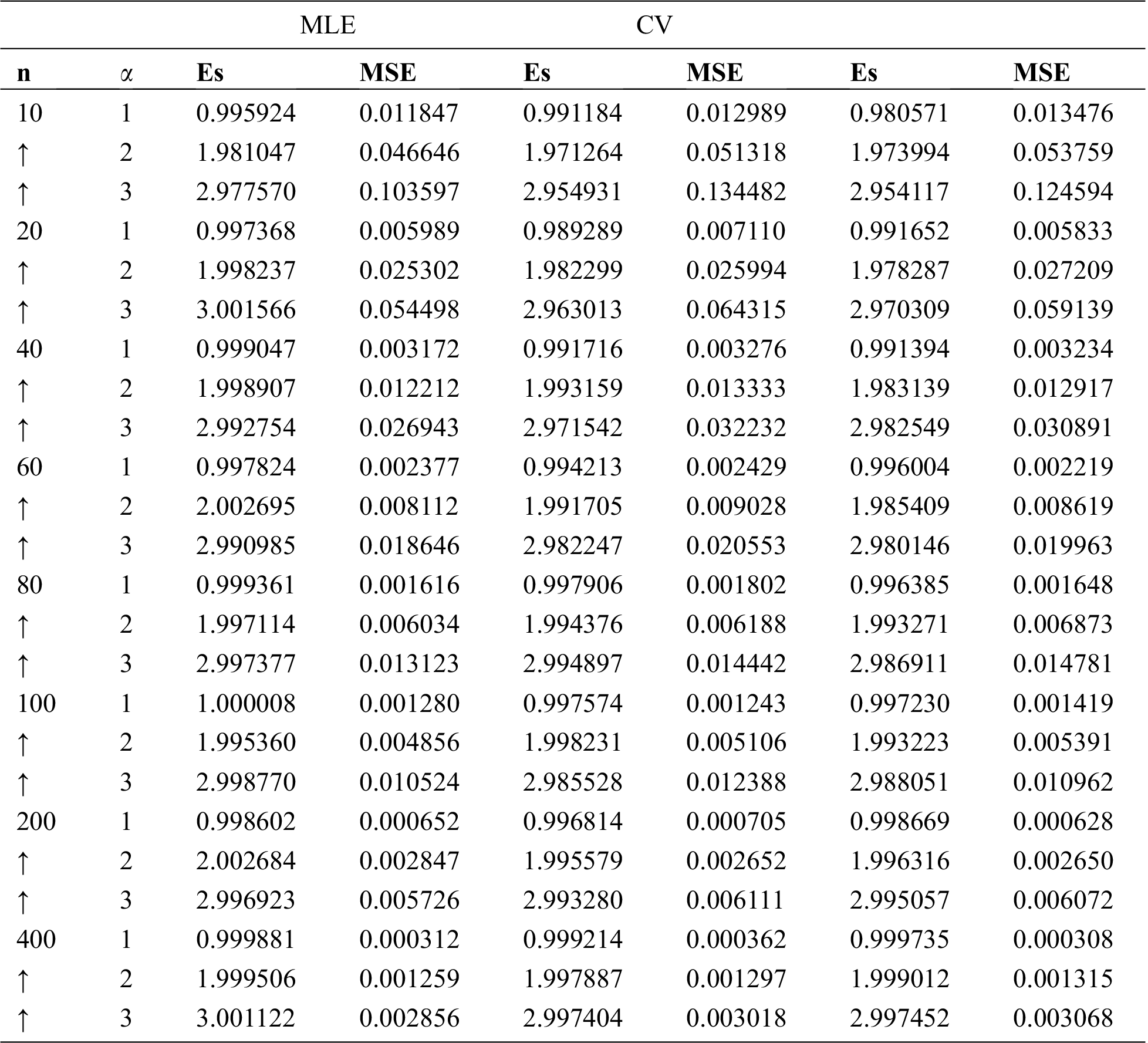
Table 2: Estimates and MSEs with LS, WLS, and MPS methods for the ILBMD with $α=1,$ 2,3 and $n=10,$ 20,40, 60, 80, 100, 200, 400

images

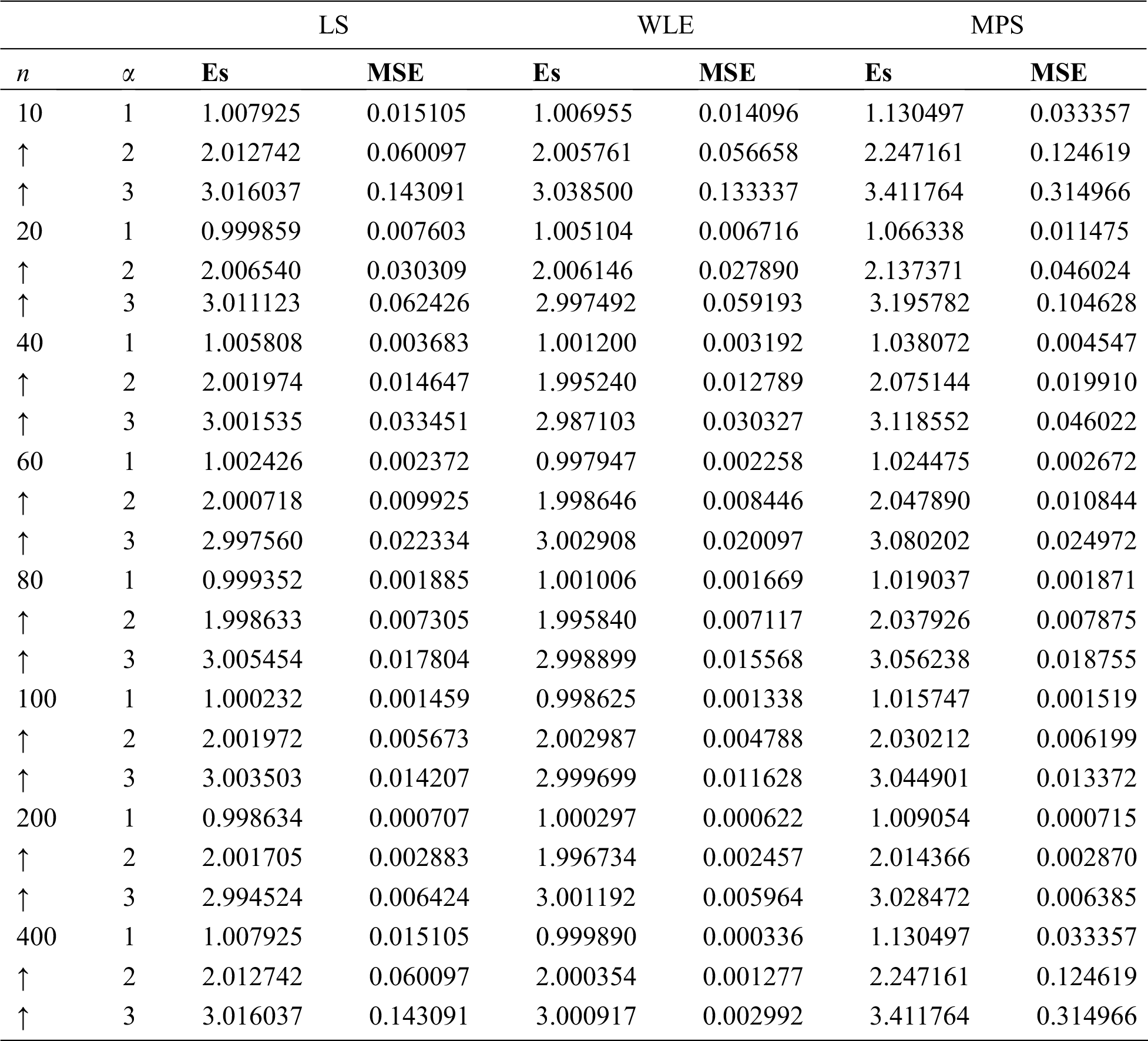
The bias of the suggested estimators is very small and goes to zero for all cases considered in this study. Also, as the samples sizes increase the MSE of all proposed estimators decreases.

6 Real Data Application

In this section, we use lifetime data set to compare the fit of the suggested ILBMD distribution with four competitors distributions: Rani, length-biased Maxwell distribution, Rama, and exponential defined as

1) Rani distribution (Rn) suggested by Shanker et al. [23] with pdf given by

$f(x;α)=α5α5+24(α+x4)e−αx;α>0,x>0$ .

2) Length-biased Maxwell distribution (LBM), $f(x;α)=12α4x3e−x22α2;α>0,x>0.$

3) Rama distribution (Rm) suggested by Gross et al. [24] with pdf given by

$fRD(x;α)=α4α3+6(x3+1)e−αx$ $x>0,α>0.$

4) Exponential distribution (Exp), $f(x;α)=αe−αx;x>0,α>0.$

The data set given in this section represents the relief times of 20 patients receiving an analgesic. This data set was taken from [25] and it is: 1.1, 1.4, 1.3, 1.7, 1.9, 1.8, 1.6, 2.2, 1.7, 2.7, 4.1, 1.8 ,1.5, 1.2, 1.4, 3.0, 1.7, 2.3, 1.6, 2.0.

In order to compare the two models, we consider the Akaike Information Criterion (AIC), Consistent Akaike Information Criterion (CAIC), Hannan-Quinn Information Criterion (HQIC), and Bayesian Information Criterion (BIC). The generic formulas for finding AIC, CAIC, HQIC, and BIC are respectively, given as $AIC=−2log⁡L+2m,$ $CAIC=−2log⁡L+2mnn−m−1,$ $BIC=−2log⁡L+κlog⁡(n),$ $HQIC=2log⁡{log⁡(n)[m−2log⁡L]}$ , where -2logL is the negative maximized log-likelihood values. The Kolmogorov-Smirnov (K-S) test statistic where these measures are defined as $KS=Supn|Fn(x)−F(x)|$ , where $Fn(x)=1n∑i=1nIxi≤x$ and $m$ is the number of parameters and n is the sample size. Also, the Kolmogorov-Smirnov (KS) test is empirical distribution function and $F(x)$ is cumulative distribution function. The best distribution corresponds to lower values of -2lnL, AIC, AICC, BIC, HIQC and KS statistic. The results are displayed in Tab. 3.

Table 3: Model comparison using AIC, CAIC, BIC, HQIC, -2logL, and the KS test criterion for the 20 patients data

images

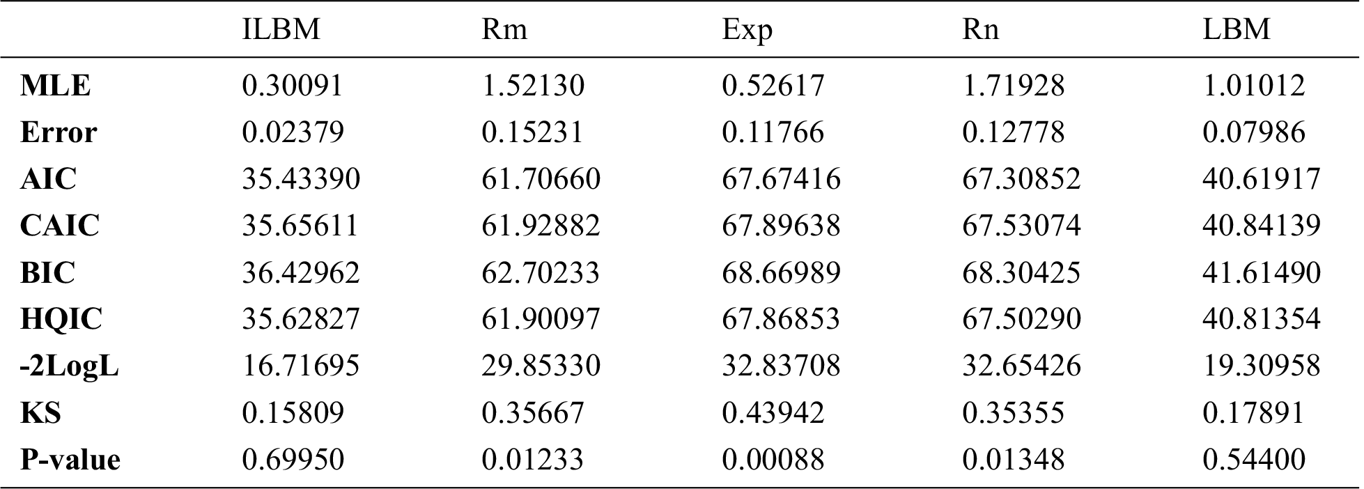
Hence, we can deduce that the inverse length biased Maxwell distribution leads to a better fit than the Rama, Rani, length biased Maxwell and exponential distribution. The Kolmogorov Smirnov p-value suggests that inverse length biased Maxwell distribution fits statistically better than other distributions considered in this example to the 20 patients data set. Plots of the fitted densities and the histogram are given in Fig. 4.

images

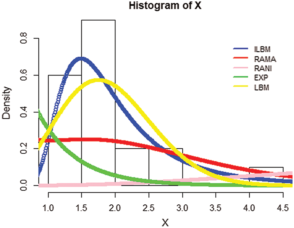
Figure 4: The fitted pdfs of the Rama, Rani, LBM, Exp and ILBM models

7 Conclusions

In this article, we introduced and studied the ILBMD. Some statistical properties of the ILBMD are derived and discussed. The reliability and hazard functions of the distribution are analyzed. Also, the distribution of order statistics, mode, harmonic mean, Fisher's information, the stochastic ordering and the mean deviations about the mean and median are presented. The distribution parameter is estimated using different estimation methods includes the maximum likelihood estimation, method of moments, maximum product of spacing, ordinary and weight least square procedures, and the Cramer-Von-Mises methods. The q and Rényi entropies are derived as well as the stress strength reliability is obtained. A real data sets is considered to support the paper objectives. It is revealed that the ILBMD is more power than its competitors used in this study. As a future works the distribution parameter can be estimated based on ranked set sampling method, see [26–32].

Acknowledgement: The authors are grateful to the Editor and anonymous reviewers for their valuable comments and suggestions.

Funding Statement: A.R.A. Alanzi would like to thank the Deanship of Scientific Research at Majmaah University for financial support and encouragement.

Conflicts of Interest: The authors declare that they have no conflicts of interest.

References

1. Y. A. Iriarte, J. M. Astorga, H. Bolfarine, H. W. Gómez et al., “Gamma-Maxwell distribution,” Communications in Statistics - Theory and Methods, vol. 46, no. 9, pp. 4264–4274, 2016. [Google Scholar]

2. J. Huang and S. Chen, “Tail behavior of the generalized Maxwell distribution,” Communications in Statistics-Theory and Methods, vol. 45, no. 14, pp. 4230–4236, 2016. [Google Scholar]

3. A. Saghir, A. Khadim and Z. Lin, “The Maxwell length-biased distribution: Properties and estimation,” Journal of Statistical Theory and Practice, vol. 11, no. 1, pp. 26–40, 2016. [Google Scholar]

4. C. R. Rao, J. Mathew and C. Chesneau, “On discrete distributions arising out of methods of ascertainment,” Sankhya: The Indian Journal Statististical Series A, vol. 27, pp. 311–324, 1965. [Google Scholar]

5. J. Mathew and C. Chesneau, “On discrete distributions arising out of methods of ascertainment,” Mathematical and Computational Applications, vol. 25, no. 4, pp. 1–21, 2020. [Google Scholar]

6. K. Modi and V. Gill, “Length-biased weighted Maxwell distribution,” Pakistan Journal of Statistics and Operation Research, vol. 11, no. 4, pp. 465–472, 2015. [Google Scholar]

7. K. L. Singh and K. L. Srivastava, “Estimation of the parameter in the size-biased inverse Maxwell distribution,” International Journal of Statistika and Mathematika, vol. 10, no. 3, pp. 52–55, 2014. [Google Scholar]

8. A. I. Al-Omari, A. D. Al-Nasser and E. Ciavolino, “A size-biased Ishita distribution and application to real data,” Quality & Quantity, vol. 53, no. 1, pp. 493–512, 2019. [Google Scholar]

9. M. Garaibah and A. I. Al-Omari, “Transmuted Ishita distribution and its applications,” Journal of Statistics Applications & Probability, vol. 8, no. 2, pp. 67–81, 2019. [Google Scholar]

10. R. M. Usman, M. A. Haq, S. Hashmi and A. I. Al-Omari, “The Marshall-Olkin length-biased exponential distribution and its applications,” Journal of King Saud University - Science, vol. 31, no. 2, pp. 246–251, 2019. [Google Scholar]

11. D. H. Shraa and A. I. Al-Omari, “Darna distribution: Properties and applications,” Electronic Journal of Applied Statistical Analysis, vol. 12, no. , pp. 520–541, 2019. [Google Scholar]

12. A. I. Al-Omari and I. K. Alsmairan, “Length-biased Suja distribution: Properties and application,” Journal of Applied Probability and Statistics, vol. 14, no. 3, pp. 95–116, 2019. [Google Scholar]

13. K. M. Alhyasat, K. Ibrahim, A. I. Al-Omari and M. A. Abu Baker, “Power size biased two-parameter Akash distribution,” Statistics in Transition New Series, vol. 21, no. 3, pp. 73–91, 2020. [Google Scholar]

14. V. K. Sharma, S. Dey, S. K. Singh and U. Manzoor, “On length and area biased Maxwell distributions,” Communications in Statistics - Simulation and Computation, vol. 47, no. 5, pp. 1506–1528, 2018. [Google Scholar]

15. A. I. Al-Omari and M. Gharaibeh, “Topp-Leone Mukherjee-Islam distribution: Properties and applications,” Pakistan Journal of Statistics, vol. 34, no. 6, pp. 479–494, 2018. [Google Scholar]

16. M. Gharaibeh, “Transmuted Aradhana distribution: Properties and applications,” Jordan Journal of Mathematics and Statistics, vol. 13, no. 2, pp. 287–304, 2020. [Google Scholar]

17. R. E. Glaser, “Bathtub and related failure rate characterizations,” Journal of the American Statistical Association, vol. 75, no. 371, pp. 667–672, 1980. [Google Scholar]

18. P. D. M. Macdonald, “Comment on an estimation procedure for mixtures of distributions by Choi and Bulgrem,” Journal of Royal Statistical Society, B, vol. 33, pp. 326–329, 1971. [Google Scholar]

19. J. Swain, S. Venkatraman and J. Wilson, “Least squares estimation of distribution functions in Johnson's translation system,” Journal of Statistical Computation and Simulation, vol. 29, no. 4, pp. 271–297, 1988. [Google Scholar]

20. R. C. H. Cheng and N. A. K. Amin, “Maximum product-of-spacings estimation with applications to the lognormal distribution, University of Wales IST, Math Report 79-1, 1983. [Google Scholar]

21. R. C. H. Cheng and N. A. K. Amin, “Estimating parameters in continuous univariate distributions with a shifted origin,” Journal of the Royal Statistical Society: Series B (Methodological), vol. 45, no. 3, pp. 394–403, 1983. [Google Scholar]

22. F. P. A. Coolen and M. J. Newby, “A note on the use of the product of spacings in Bayesian inference,” Technische Universiteit Eindhoven, 1990, (Memorandum COSOR; Vol. 9035). [Google Scholar]

23. R. Shanker, “Rani distribution and its application,” Biometrics & Biostatistics International Journal, vol. 6, no. 1, pp. 1–10, 2017. [Google Scholar]

24. R. Shanker, “Rama distribution and its application,” International Journal of Statistics and Applications, vol. 7, no. 1, pp. 26–35, 2017. [Google Scholar]

25. A. J. Gross and V. A. Clark, Survival distributions: Reliability applications in the biomedical sciences. New York: John Wiley and Sons, 1975. [Google Scholar]

26. A. Haq, J. Brown, E. Moltchanova and A. I. Al-Omari, “Ordered double ranked set samples and applications to inference,” American Journal of Mathematical and Management Sciences, vol. 33, no. 4, pp. 239–260, 2014. [Google Scholar]

27. A. Haq, J. Brown, E. Moltchanova and A. I. Al-Omari, “Varied L ranked set sampling scheme,” Journal of Statistical Theory and Practice, vol. 9, no. 4, pp. 741–767, 2015. [Google Scholar]

28. E. Zamanzade and A. I. Al-Omari, “New ranked set sampling for estimating the population mean and variance,” Hacettepe Journal of Mathematics and Statistics, vol. 45, no. 6, pp. 1891–1905, 2016. [Google Scholar]

29. A. Santiago, C. Bouza, J. M. Sautto and A. I. Al-Omari, “Randomized response procedure in estimating the population ratio using ranked set sampling,” Journal of Mathematics and Statistics, vol. 12, no. 2, pp. 107–114, 2016. [Google Scholar]

30. A. I. Al-Omari, “Estimation of mean based on modified robust extreme ranked set sampling,” Journal of Statistical Computation and Simulation, vol. 81, no. 8, pp. 1055–1066, 2011. [Google Scholar]

31. A. I. Al-Omari, “Ratio estimation of population mean using auxiliary information in simple random sampling and median ranked set sampling,” Statistics and Probability Letters, vol. 82, no. 11, pp. 1883–1890, 2012. [Google Scholar]

32. M. Syam, K. Ibrahim and A. I. Al-Omari, “The efficiency of stratified quartile ranked set sample in estimating the population mean,” Tamsui Oxford Journal of Information and Mathematical Sciences, vol. 28, no. 2, pp. 175–190, 2012. [Google Scholar]

This work is licensed under a Creative Commons Attribution 4.0 International License, which permits unrestricted use, distribution, and reproduction in any medium, provided the original work is properly cited.