DOI:10.32604/csse.2021.017230

| Computer Systems Science & Engineering DOI:10.32604/csse.2021.017230 |  |
| Article |
Cyclic Autoencoder for Multimodal Data Alignment Using Custom Datasets
1College of Information Engineering, Shanghai Maritime University, Shanghai, 200135, China
2Division of Management and Education, University of Pittsburgh, Bradford, 16701, USA
*Corresponding Author: Jin Liu. Email: jinliu@shmtu.edu.cn
Received: 21 January 2021; Accepted: 24 February 2021
Abstract: The subtitle recognition under multimodal data fusion in this paper aims to recognize text lines from image and audio data. Most existing multimodal fusion methods tend to be associated with pre-fusion as well as post-fusion, which is not reasonable and difficult to interpret. We believe that fusing images and audio before the decision layer, i.e., intermediate fusion, to take advantage of the complementary multimodal data, will benefit text line recognition. To this end, we propose: (i) a novel cyclic autoencoder based on convolutional neural network. The feature dimensions of the two modal data are aligned under the premise of stabilizing the compressed image features, thus the high-dimensional features of different modal data are fused at the shallow level of the model. (ii) A residual attention mechanism that helps us improve the performance of the recognition. Regions of interest in the image are enhanced and regions of disinterest are weakened, thus we can extract the features of the text regions without further increasing the depth of the model (iii) a fully convolutional network for video subtitle recognition. We choose DenseNet-121 as the backbone network for feature extraction, which effectively enabling the recognition of video subtitles in complex backgrounds. The experiments are performed on our custom datasets, and the automatic and manual evaluation results show that our method reaches the state-of-the-art.
Keywords: Deep learning; convolutional neural network; multimodal; text recognition
Nowadays, with the rise of short video in social networks, the scale of video resources has greatly increased, even beyond the scale of image data. As a kind of data that combines audio and image modalities, the video contains much more information than independent audio and image data, however, in the face of massive video data, it becomes more difficult to utilize the data of these two modalities. Video subtitles recognition is different from single-modal text recognition, although both audio sequences and text sequences contain information about a sentence, the audio is expressed in a time sequence and the text is expressed in a spatial sequence, and the dimensional sizes of the features expressed by the two modal data do not match each other.
There are similarities between the analysis of multimodal data and sentiment analysis [1–3]. Most of the existing studies on multimodal data for video data are for tasks such as video sentiment analysis, action recognition [4,5], motion prediction, video categories [6], and task tracking [7]. The above studies have something in common that the ultimate desired goal is a single classification result without temporal order characteristics, e.g., the goal of video sentiment analysis studies is to predict the emotional state conveyed in a video, and the goal of action prediction is to predict the category of action represented by the content presented in the current video clip. It is clear that the final output of the above study does not retain the original sequence information in the video, making it impossible to apply the above study method to video subtitle recognition.
Existing researches on video subtitles recognition only study the two types of data separately or uses the methods in the fields of optical character recognition (OCR) and speech recognition (ASR) to obtain the two recognition results, respectively, and perform a simple result analysis and error correction. The above-mentioned methods are not able to fully utilize multimodal data, resulting in a waste of resources. Thus, the task of studying multimodal fusion is of great practical importance.
In this paper, inspired by some articles on relationship extraction [8], complex context processing [9] and attention mechanisms [10], we will present an efficient fully convolutional network for video subtitle recognition. The cyclic autoencoder improves the performance of the model for image feature compression and solves the problem of image feature extraction. The multimodal fusion module takes full advantage of the complementary nature of the two modal data and preserves the temporal characteristics of the data. CTC (Connectionist Temporal Classification) [11] translates the output of the fully connected layer into labels.
Besides, to enhance feature extraction of audio and images, our backbone network uses a densely connected convolutional network with attentional mechanism. We evaluate our approach to custom datasets. It is observed that our method achieves promising performance. The main contributions are summarized as follows:
A residual attention module is introduced into the image feature extraction module, and the softening mask branch in the residual attention module is divided into positive and negative directions. The shallow features are analyzed through the encoder-decoder structure, which enhances the features of the image text and suppresses the interference of non-textual targets, enabling the model to extract text features more accurately.
Cyclic autoencoder based on a convolutional neural network is introduced, which enables the model to compress the image size without losing any feature information while ensuring that the compressed features still have temporal features.
Replacing recurrent neural networks with fully convolutional networks for sequence-to-sequence text line recognition of fused data, achieving good performance while solving the drawbacks of recurrent neural networks.
Before 2015, all text line recognition methods were equivalent to character recognition methods due to the lack of a good label alignment method for sequence-to-sequence recognition tasks. In 2013, Bissacco et al. [12] proposed a text line recognition model, PhotoOCR, to combine and recognize the text in an image by an over-segmentation method that The over-segmentation method slices the text lines into multiple character structures, and the fragments are combined and recognized by a Beam Search algorithm based on dynamic programming to obtain a directed graph containing the probability values of various text combinations, and the optimal path is selected as the final text recognition result. This approach is the first to consider text lines as a whole for recognition, departing from the traditional cut-and-score solution, and achieves good results on the ICDAR2013 text line recognition dataset.
In 2015, Shi et al. [13] proposed a novel model for image text line sequence recognition called Convolutional Recurrent Neural Network (CRNN), by combining Deep Convolutional Neural Network (DCNN) [14], Recurrent Neural Network (RNN) [15] and a label alignment algorithm called Connectionist Temporal Classification (CTC) allows the model to directly use text sequence labels for end-to-end learning. By using a DCNN, the feature representation in the image data can be learned directly without manual feature extraction and pre-processing steps, while by adding an RNN model after the DCNN model, the model can capture the contextual information implied in the image features to achieve a more stable text sequence recognition. Besides, thanks to the properties of both structures, the model only needs to restrict the image height during the training and testing phases and the length of the input text sequence can be arbitrary.
The study of multimodal learning began in the 1970s, great breakthroughs have taken place in this field after deep learning is put forward in the 21st century. Nowadays, there are four main research directions in multimodal learning: data modal mapping transformation, data modal alignment, multimodal data fusion, multimodal data collaboration.
In 2018, Audebert et al. [16] proposed a model based on multiscale image semantic segmentation for the delineation of the street, pavement, and water boundaries for urban overhead views. They set up two different ways to fuse the city top view with the satellite remote sensing map, pre-fusion, and post-fusion. In this way, they investigate the performance differences of different fusion methods on the final semantic segmentation results of the model. The experiments prove that although the performance of the model can be greatly improved by the pre-fusion method, the model's immunity to noise is not as expected, while the post-fusion can compensate for the effects of errors and gaps in the data and is robust to noisy data.
The study of multimodal data fusion has received extensive attention from scholars at home and abroad in recent years. The application of video data is an important scenario for multimodal data fusion research. Video data often contain implicit modal data such as audio, images, frame sequences, language models, subtitles, etc., which can be used for sentiment analysis, video categorization, caption recognition, and other various research tasks. Fukui et al. [17] argued that in a visual quizzing task, the representation vector of video data with text data is used directly multimodal pooling methods that multiply or add at the elemental level do not produce sufficient feature expressions to achieve the task goal, so they proposed a bilinear pooling method for multimodal data, which can combine and express these two modal features efficiently. And it achieves optimal performance in a visual question-and-answer task in the Visual7W dataset.
In 2019, Yu et al. [18] proposed a general uniformity attention mechanism for capturing the feature interaction expression within and between modal. By applying this attentional mechanism to their multimodal network model further enhances the visual quizzing task's ability to achieve the optimal performance.
In 2018, on the task of fraud detection in video, Krishnamurthy et al. [19] proposed a multimodal learning approach based on deep learning. By using different neural network models to extract features from video, audio, facial expression, and text, respectively, and abstracting the data to one-dimensional vectors, then representing vectors of different modal features are directly stitched together and input to the fully connected network for classification of the results. This method achieves better performance, but the operation of flattening the features results in a loss of spatial information in the features, which affects results. This problem was addressed to some extent by Poria et al. [20], who applied multimodal data fusion to video in sentiment analysis. They eliminated the spreading part of the merged model and instead made the extracted features have the same size in the channel dimension by pre-set parameters, and then cascaded the individual features in the channel dimension for stitching and input into the classification. In 2019, Majumder et al. [21] further optimized their model based on this study. The fusion of the model was divided into multiple levels, with the three expression level features first entered two by two into the bimodal fusion model, and then the obtained deep features are further input into the three-modal fusion model to obtain the final fusion features for sentiment classification. Compared with existing state-of-the-art models, the accuracy of their model improved by 1 to 2 percentage points.
In this section, we first introduce the architecture of the proposed fully convolutional network for video subtitles recognition. Then, we will describe each component in detail.
The overview of our fully convolutional network is illustrated in Fig. 1, composed of a cyclic autoencoder, multimodal data fusion module, and a CTC (Connectionist Temporal Classification) module.
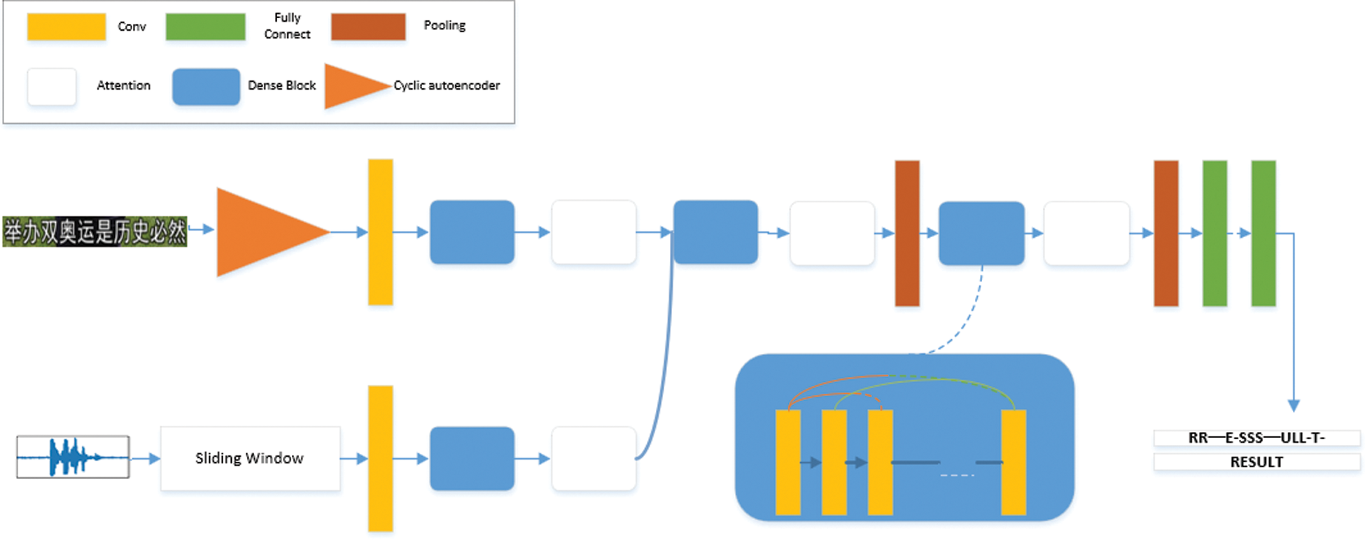
Figure 1: Network structure of our fully convolutional sequence modeling
The formal definition of a caption recognition task based on multimodal data fusion is as follows, assuming a grayscale input of an image with height H and width W:
An audio input with a duration of T seconds and a sample rate of P is:
The final output of the model is a sequence of text results:
For preprocessing, the audio is converted to mono and the sampling frequency of the audio is fixed, then the audio is converted to a spectrum using a sliding window and the Short Time Fourier Transform (STFT) is computed for the audio. A cyclic autoencoder is introduced in the feature compression section, which enables the model to compress the original image features non-equally without losing any feature information while ensuring that the compressed features are still temporally sequential. The features of the multimodal data in the feature extraction layer are each entered into the cyclic self-encoder to obtain features of equal length, and then the two features are concatenated on the channel dimension, each column in the sequence is separately inputted to the full connection layer for classification. We use CTC as the final loss function to obtain sequence identification results.
The traditional method of image scaling to compress the image is likely to lead to a large loss of image information, making image feature extraction difficult [22,23]. The most commonly used feature compression method today is autoencoder. The autoencoder is a network model for compressing the feature vector dimensions, which consists of an encoder and a decoder. The input content of the model is labeled as the true value of the output content, and then through unsupervised learning, the model is enabled to learn the given Patterns of data hidden in feature vectors to eliminate redundancy and dimensionality reduction of data features.
Assume that the input image to be compressed is:
Where i and j represent the length and width of the image. The resulting output is given as:
Where k, l stands for the length and width of the output image, it should be noted that the length and width of the output image should be smaller than the input image, and the size of the output image varies with the input.
The autoencoder is defined formally as follows, assuming the input feature vector is:
Where d is the dimension of the input vector and assumes that the output feature vector is:
Where e is the hidden layer feature vector dimension. Our goal is to find a mapping function Ed,e (x) such that:
The features of the input vector are preserved as much as possible while the dimension of the output vector is smaller than the dimension of the input vector.
The ultimate goal is to be able to obtain a mapping function Ed,e (x) of the encoder that projects the input to the hidden layer and allows the feature vector reconstructed by the mapping function
As shown in Fig. 2 (left), the autoencoder is able to compress the dimensions of the feature vector well, however, the model has several shortcomings: (i). The autoencoder's intermediate hidden layer must have fewer feature vectors than the dimensions of the input features, as the autoencoder will only copy the original data. (ii) The feature vectors learned by the autoencoder do not necessarily preserve the spatial structural properties of the input feature vectors, due to the structural nature of fully connected neural networks that result in connections between network layers that are not locally sensitive. As shown in Fig. 2 (right), autoencoder based on convolutional neural network with local connections using convolutional operation both reduce the model training parameters and ensure that the compressed feature vector continues to maintain its original temporal characteristics, which is a good solution to the second shortcoming of the autoencoder. However, the first defect is still not solved, and the compression ratio of the feature vector is still insufficient, making it impossible for the two modal data to be aligned.
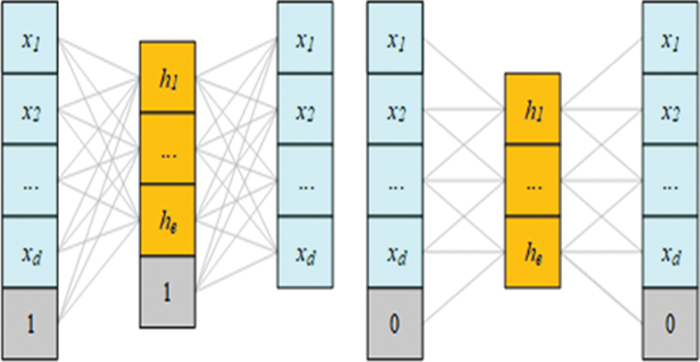
Figure 2: Model structure of autoencoder (left) and autoencoder based on convolutional neural network (right)
To address the above existing problems, this paper proposes a cyclic autoencoder based on convolutional neural network. Our model learns patterns from the input data, records the pattern features from the previous round of training, and applies them to the next round of training, enabling the model to learn information that was missed in the previous round, thus allowing the two modalities of data to be aligned separately in terms of feature dimensions. Our cyclic autoencoder also improves the performance of image feature compression, making the model more flexible and adaptable.
The form of the model is defined below:
Our cyclic autoencoder is shown in Fig. 3. The model consists of two parts, the encoder consists of two dense blocks and a convolutional layer with a stride 1x2. The size of the convolution kernel in both convolutional layers is 3 × 3. The stride of the convolutional operation is set to 2. The formula for calculating the output size of a convolutional operation is as follows.
Where
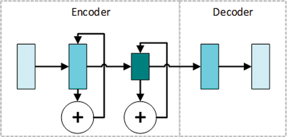
Figure 3: Cyclic autoencoder network diagram
The output size of each network layer is half of the input size, which makes the network layer in a way that produces a pooling effect of It also does not ignore any information in the input features. Also, our encoder that uses convolution operation with a stride of 2 has a smaller computation than a conventional encoder. The length and width of the feature map obtained from the encoder part are 1/4 of the original input image, which means that the compression ratio of the image can reach 1:16.
Moreover, the number of convolutional kernels in each convolutional layer is the sum of the number of convolutional kernels in the current round and the number of convolutional kernels in the previous round. That is, assuming that the preset number of convolutional kernels in a single round is k when in the i-th round of training, then the number of convolutional kernels in the current convolutional layer is i*k. However, not all of the convolutional kernel parameters need to be trained, because training in the previous i-1 rounds yielded the convolutional kernel parameters are already sufficient to express part of the image pattern information. Thus there are only k convolutional kernels that can be modified in the i-th round of training. To be able to stop the training at the appropriate time, we set a termination condition for the model's training. Training is stopped when the accuracy of the model in the validation set reaches 98% or more.
Since our ultimate goal is to be able to stably compress the features of the image without the need to restore the compressed data, after training, only the parameters of the convolution kernel of the encoder will be left and merged into the subsequent modules, and the parameters of the decoder will simply be discarded.
We expand the cyclic autoencoder by timeline, as shown in Fig. 4. Each dashed box represents a complete cyclic autoencoder structure, and the light blue rectangles in the dashed boxes represent the input and output. Since the compression performance of autoencoder is judged by whether the model's output can be kept in line with the input, therefore the true value image used in training the model should be the input image. From left to right, the number of training rounds increases, the connecting line between the two dashed boxes represents the concatenating of the parameters of the convolutional layer and sets this part of the convolutional kernel to not train. Training is stopped when it reaches the number of rounds of the pre-training setup or the termination condition we set. The advantage of cyclic training is the ability to increase the channel dimension of the intermediate feature vector while ensuring that the available intermediate vector dimension is less than the input dimension of the vector dimension of the feature.
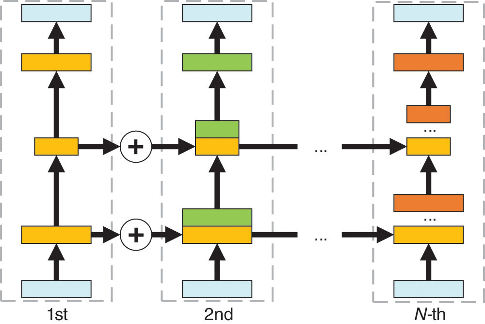
Figure 4: The unrolled diagram of our cyclic autoencoder by time line
3.3 Bi-direction Residual Attention Module
He et al. [24] proposed a network structure called residual module to improve the training method of the network and solve the degradation problem. First of all, assuming that there is a neural network with fewer layers that have reached the saturation accuracy, then adding multiple identity mapping layers (identity mapping, i.e., y = x) after it will not affect the accuracy. In this way, while increasing the number of network layers, at least it will not reduce the accuracy. The important inspiration of the residual module comes from the idea of using the identity mapping to directly pass the output of the previous layer to the back layer. The structure of the residual module is in Fig. 5:
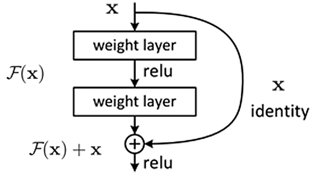
Figure 5: The Structure of Residual Module
Assuming that the current layer input of the neural network is x, and the expected output is, according to the above, when the accuracy rate is close to saturation, the current learning goal will be converted into an identity map, so that the degradation problem will not lead to accuracy decline. According to the structure diagram of the residual module in Fig. 5, we directly take the input x as the initial value of the output and define the final output value as. It can be found that when, the entire map is transformed into an identity map. Using this method to define the output value of the network layer, the learning goal of the network layer will be converted into the difference between the target value and the input, which is also the origin of the term residual. At this time, the training goal of the network becomes to make close to 0. The proposed residual module effectively solves the degradation problem caused by too many network layers and brings the possibility of training ultra-deep networks with large network depth.
To enable the text detection model to have a certain sensitivity to the target semantic information in the shallow features of the feature extractor. We introduce a new attention mechanism to strengthen the regions of interest in the image and weaken the regions of non-interest so that we can improve the performance of the model in extracting the features of the text area without further increasing the depth of the model. BRAM adds two new soft mask branches based on the original image feature forward branch: forward soft mask branch and negative soft mask branch. Assuming that the attention mechanism module is in the two neural network layers, x represents the feature input of the previous network layer,
Where i is the product of the height and width of the input feature, representing the spatial coordinate value in the specified input feature. c represents the channel position in the input feature.
The bidirectional residual attention module is usually added in the middle of two adjacent convolutional neural network layers. Namely, the feature input received by the module and the feature output provided by the module should have the same size in the length and width dimensions.
The structure of the module is shown in Fig. 6. The yellow dotted box is the overall structure of the two-way residual attention mechanism. The module has three branches in total: the main branch, the forward soft mask branch, and the negative soft mask branch. The main branch can be simplified as a basic residual convolution block, which contains t layers of residual convolution units. Without considering the influence of the two soft mask branches, the module can directly implement the most common image feature extraction function. The two soft mask branches are roughly the same in structure and are composed of an encoder-decoder based on the residual block. The difference is that the mask results obtained by the two branches respectively enhance and suppress the feature maps in the main branch, which makes the representation of the feature map clearer.
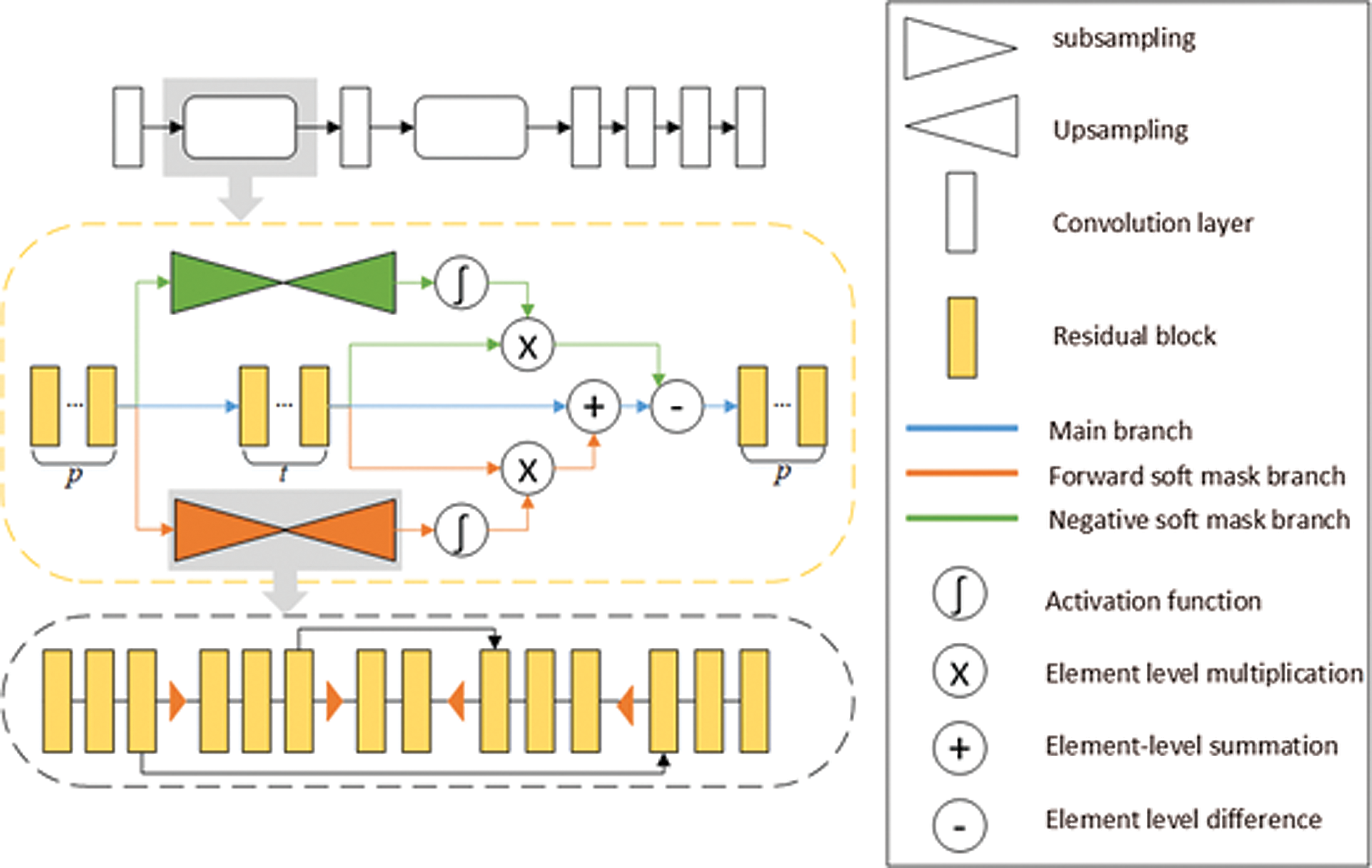
Figure 6: Bi-direction residual attention module
This module contains two hyperparameters that can be selected and set, p represents the number of residual blocks that serve as a buffer before and after the attention module, and t represents the number of residual blocks that need to be extracted in the main branch.
The model structure of the early image text sequence prediction is shown in Fig. 7. The images are the first feature extracted by a convolutional neural network, and then the obtained feature map is expanded in columns to obtain the set of feature vectors and input to a derivative network such as RNN or LSTM [25]. However, since recurrent neural networks are used in the model to predict sequences, there is an inevitable need to address the problems: The model cannot be trained in parallel, and the training process is prone to gradient disappearance and gradient explosion problems. To solve some of the above problems, this paper proposes a text line sequence recognition model based on the fully convolutional network. By replacing the original recurrent neural network with a convolutional neural network layer, the problem is eliminated while maintaining the original prediction performance.
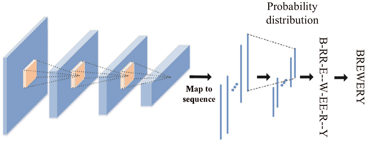
Figure 7: Early text line sequence recognition models
The most representative network in the field of computer vision is the convolutional neural network. Based on the fact that convolutional kernels have local connections, the network model computes the features of each pixel from the surrounding neighboring pixels, making the convolutional neural network context-sensitive, which varies with the size of the convolutional kernel, in line with our needs for sequence-to-sequence text image recognition tasks and speech recognition tasks. Therefore, this paper replaces the original recurrent neural network model with a convolutional neural network and shows that densely connected convolutional neural networks perform modeling of feature classification.
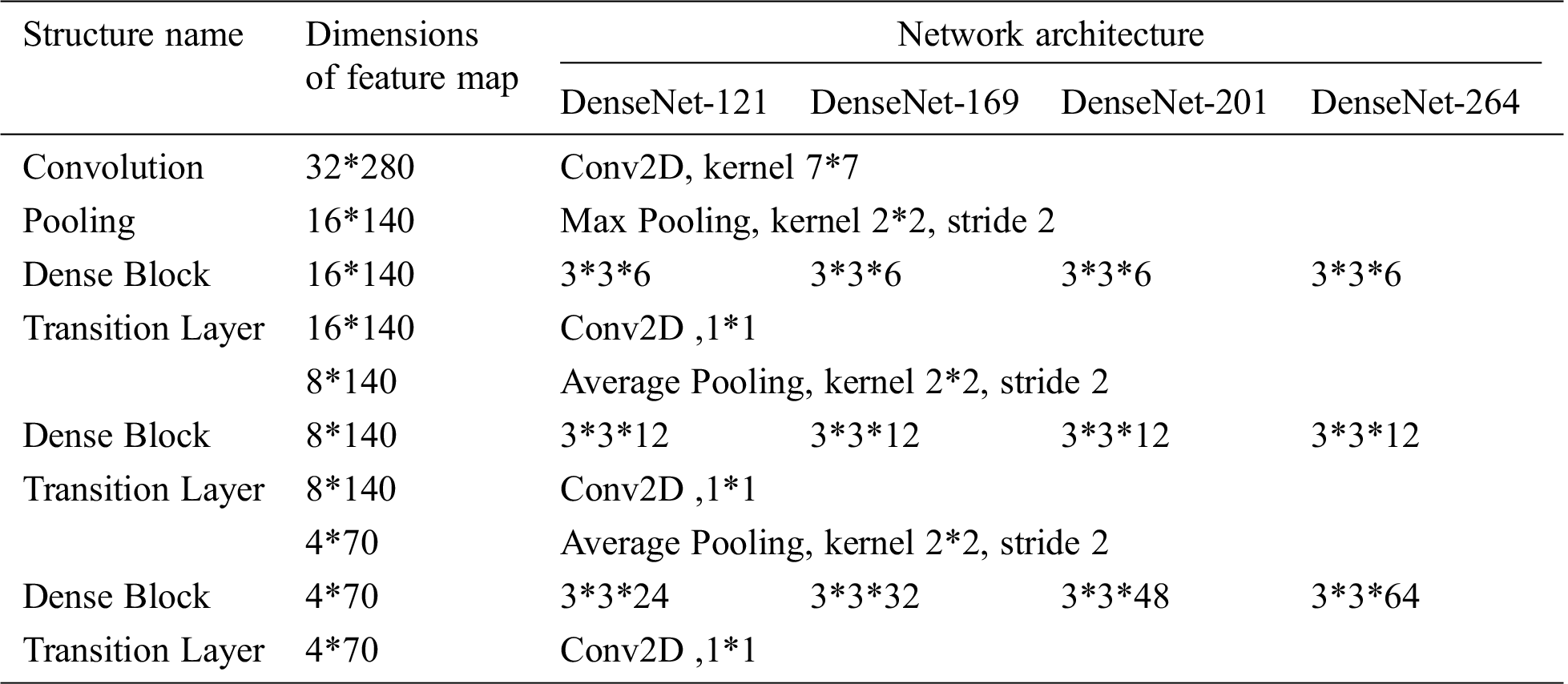
DenseNet's [26] model architecture connects all layers directly to each other to ensure maximum information flow between the network layers. To maintain the feedforward feature, each layer will get additional input from all previous layers and pass its feature map to all the subsequent layers. Because of the densely connected nature, this network structure obtains shallow image morphological features by accepting additional input from the preceding network layer without learning redundant feature maps. In this paper, the densely connected convolutional network structure is used to solve the feature learning redundancy problem of the VGG16 model, and also to solve the problem that the shallow features are not well represented in the residual neural network due to the direct summation of the features.
The dimensionality of the input features can be very high since the input of each layer in a dense convolutional block contains the output of each preceding layer. To be able to downscale the input features, the network adopts a structure similar to the bottleneck layer in a residual network. The bottleneck layer is implemented as a 1 × 1 convolution of the input features, which greatly reduces the number of parameters in the model structure.

Figure 8: Densely Connected Convolutional Network
Table 1: Parameters of Commonly Used Densely Connected Network
In order to verify the feasibility and validity of our proposed model, we have made the following experiments.
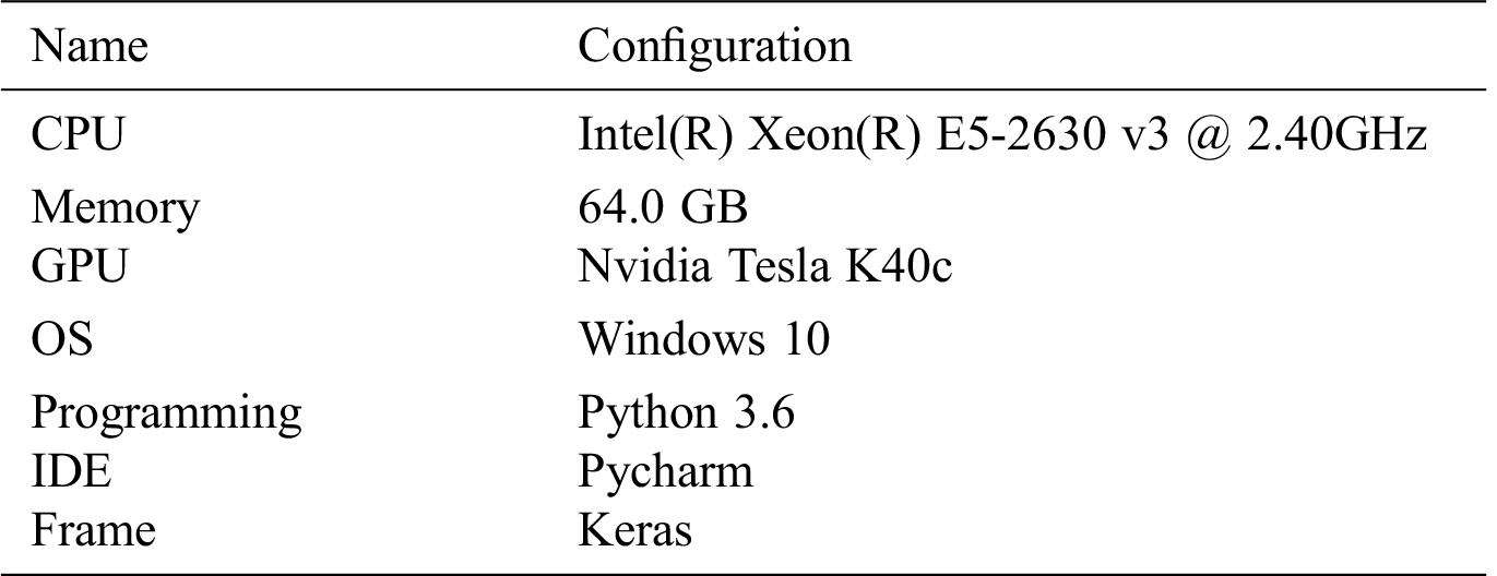
Our experimental environment and configuration are shown in Tab. 2.
Table 2: Experimental Environment Configuration
Existing multimodal datasets for text recognition are typically video-audio modal datasets, which are currently audio-image modal datasets still does not exist, so we have designed a production flow for the audio-image modal dataset. And the experimental datasets required for this chapter were generated based on this production flow.
The Fig. 9 shows a flowchart for the production of an audio-image modal dataset, with the two sides of the dotted line representing the two methods of producing the two datasets. The left side of the dashed line is plotted by plotting the corresponding textual truth values of the audio into the natural scene image. The right side of the dashed line is used to distinguish the time frame positions of the corresponding subtitles in the video by detecting the cut of the audio endpoints and using the OCR tool extracts and identifies the subtitles, and then merges them with the corresponding audio to generate a training data set.
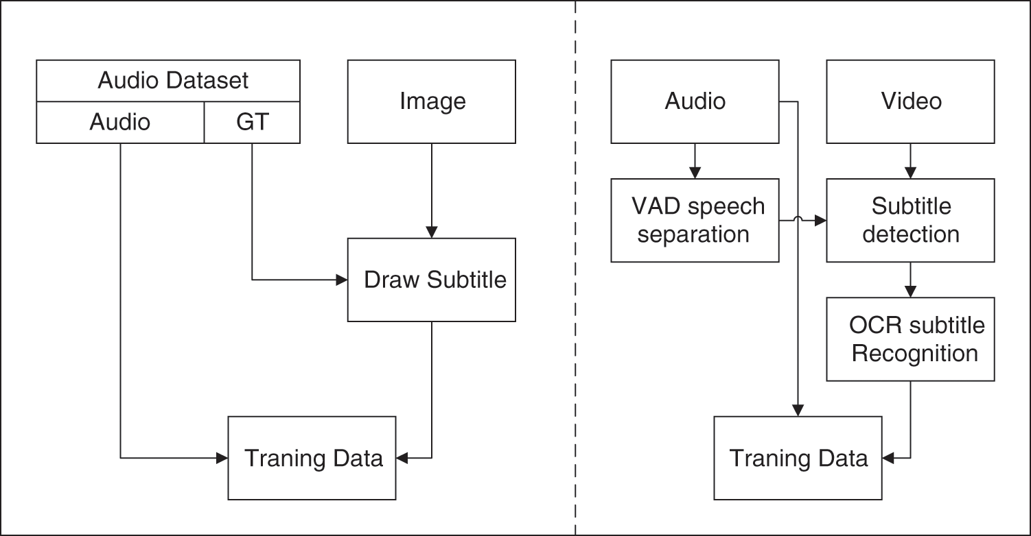
Figure 9: Audio-image Modal Video Subtitle Dataset
In the first method of creating a dataset, we use the audio counterpart's textual content as a dataset by plotting it in a natural scene image. We selected AISHELL-ASR0009-OS1, a Chinese Mandarin open-source speech database by Hill Shell. The dataset contains 400 speakers from different accent regions in China who participated in the recording. In the caption recognition experiment, we plotted the captions on the COCO dataset to generate a new video caption dataset. The COCO dataset is a realistic, publicly available dataset from Microsoft for tasks such as target detection, semantic segmentation, and image classification. The scene image dataset, which contains a total of 82,783 images, and annotations for target detection and semantic segmentation Results.
The text’s true values corresponding to the audio are plotted anywhere in the image of the complex scene image dataset COCO, and the obtained text lines are cut to obtain the text line image data for complex scenes. Besides, in order to ensure that the image and audio branches do not conflict with each other in terms of missing obscure characters, we unify the two sides' font size. Since the text in the resulting text line image is still a standard text image, to be able to test the generality of the model, we Further transformations such as zooming, panning, rotating, and distorting text lines are performed by affine transformations. Additional operations to add noise, smudge, and blocking to the image are also applied to our dataset. A partial sample of the final generated dataset is shown in Fig. 10.
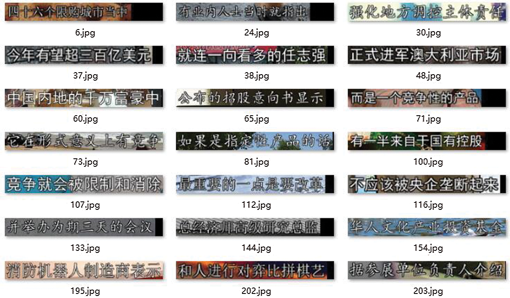
Figure 10: Video caption dataset
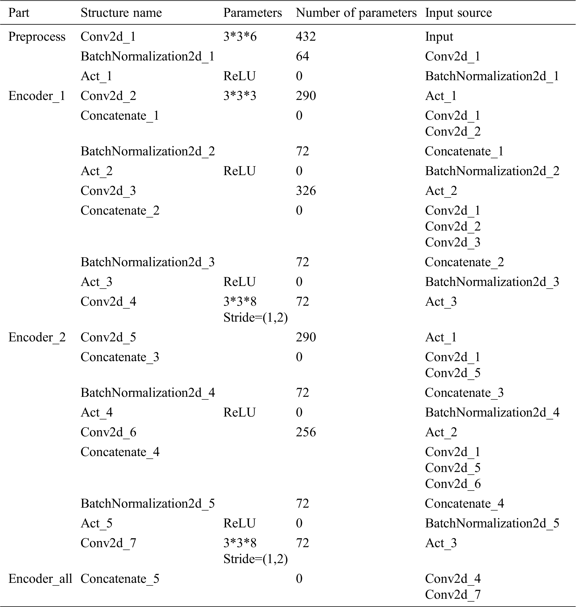
To demonstrate that cyclic autoencoder is capable of low-loss, non-equally proportional compression of images, we use 3 × 3 sized convolutional kernels (16 in total), perform convolution on the subtitle images, and then input the resulting features to the encoding structure in the cyclic autoencoder. Due to an inherent flaw in the Keras, stitching the convolutional layers of each round of encoders into a new convolutional layer is difficult, and we can achieve the same result by concatenating the convolution results from different rounds in the channel dimension. To be able to illustrate in detail how the feature size varies in the model, we assume that the model is only trained for 2 rounds, and the detailed parameters of the coding structure in the model are presented in Tab. 3.
Table 3: Parameters of Network Model Structure in the Second Round of Training
We trained the cyclic autoencoder for a total of 450 iterations over 20 rounds using the above experimental setup, and the training and validation results recorded during the training process are shown in Fig. 11 below.
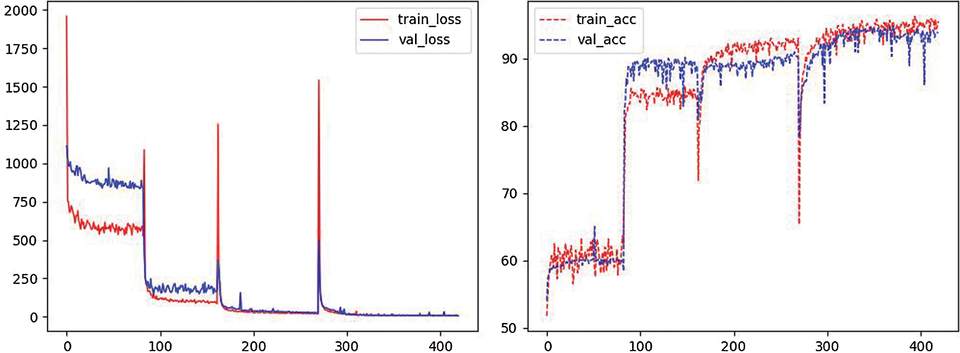
Figure 11: Training process of cyclic autoencoder
As shown in Fig. 11, four distinct spans in the variation of the curve, which is because the fact that every five iterations, a new encoder structure is added to the cyclic autoencoder. Since the emerging structure has not yet been trained, the loss value initially rises, but then quickly drops and does not have an impact.
From Fig. 12, we can see that even if the image size is compressed to 1/6th of the original size, we can still achieve nearly 60% accuracy after reduction to the original size, and as the number of compressed feature channel dimensions increases, the trend of increasing accuracy gradually slows down, indicating that our cyclic autoencoder has already learned most of the features of the pattern in the image at the early stage, and subsequent learning is learning deeper features that were not learned previously.
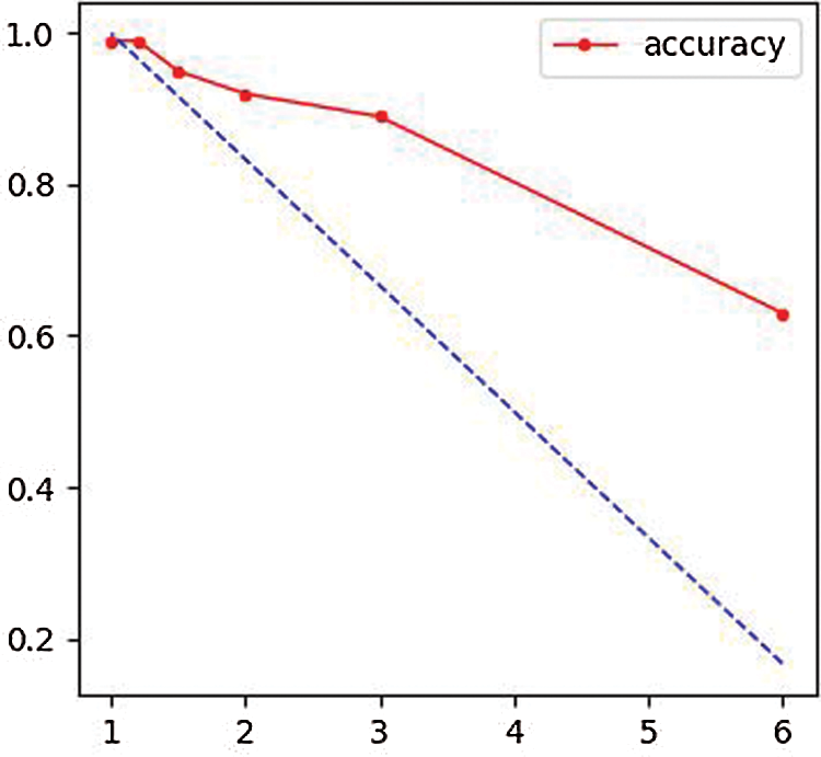
Figure 12: Accuracy at different compression ratios of the cycle autoencoder
We need to reproduce the current best performing method and test it on our dataset, this research method is more time consuming but has the advantage of being able to compare on the same computer hardware environment.
The evaluation criteria used in the text recognition task in this paper are sentence accuracy and soft accuracy. There is no difference between the calculation method of the two indicators and the ordinary accuracy calculation method. The difference between the two is that the positive sample judgment for sentence accuracy is based on whether all characters in a text line are correctly classified, while the positive sample judgment for word accuracy is based on whether all characters are correctly classified.
In Fig. 13, red markers indicate that the text was not recognized, blue markers indicate that the text recognition result does not exist in the true value, and green markers indicate misrecognition.

Figure 13: Identification results of different methods on test data samples
Tab. 4 shows the best performance of each method on our custom datasets. We have finally selected 15 methods for our model performance comparison experiments.
Table 4: Performance comparison results
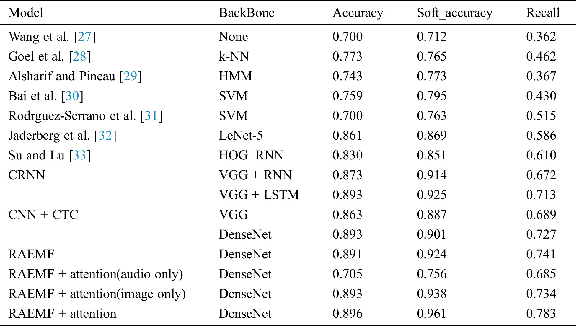
As can be seen from Fig. 14, the accuracy rate at the level of text lines does not open up a big gap between each method, but our method still has some advantages over the other methods. Besides, to prove that using multi-modal data for text line recognition can achieve the performance that cannot be achieved by using the two modal data alone. The results show that the performance achieved by using the image data alone is at most on par with the best available method, while the audio data alone is far below our expected performance index. Therefore, the fusion of audio and image data can indeed bring richer features to the model, and can also effectively improve the model's recognition performance for textual line sequences.
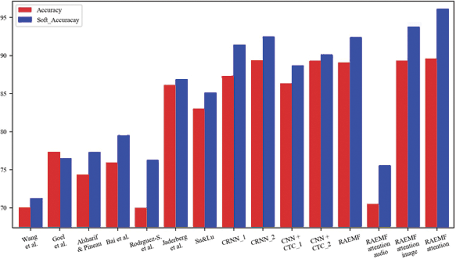
Figure 14: Visualization of model experiment comparison results
In this paper, we propose a novel fully convolutional network for video subtitle recognition, which addresses the existing problem that the dimensional sizes of image data and audio data do not match at all. Cyclic autoencoder based on a convolutional neural network is introduced, which enables the model to compress the image size without losing any feature information while ensuring that the compressed features still have temporal features. By inputting the features of the image and audio modal data outputted from the feature extraction layer to the cyclic autoencoder respectively, the features of equal length are obtained, and then the two features are concatenated in the channel dimension and then each column of the sequence is inputted to the full connection layer for identification. The final sequence identification is obtained using the CTC (Connectionist Temporal Classification) as the final loss function. Our method can deal with video caption recognition in complex scenarios. The extensive experimental results on the custom datasets demonstrate the superiority of our approach compared with the state-of-the-art.
Conflicts of Interest: The authors declare that they have no conflicts of interest to report regarding the present study.
Funding Statement: This work is supported by the National Natural Science Foundation of China (61872231).
1. J. Zeng, Y. Dai, F. Li, J. Wang and A. K. Sangaiah, “Aspect based sentiment analysis by a linguistically regularized CNN with gated mechanism,” Journal of Intelligent & Fuzzy Systems, vol. 36, no. 5, pp. 3971–3980, 2019. [Google Scholar]
2. F. Xu, X. Zhang, Z. Xin and A. Yang, “Investigation on the Chinese text sentiment analysis based on convolutional neural networks in deep learning,” Computers, Materials & Continua, vol. 58, no. 3, pp. 697–709, 2019. [Google Scholar]
3. P. Cen, K. X. Zhang and D. S. Zheng, “Sentiment analysis using deep learning,” Journal on Artificial Intelligence, vol. 2, no. 1, pp. 17–27, 2020. [Google Scholar]
4. C. Zhu, Y. K. Wang, D. B. Pu, M. Qi, H. Sun et al., “Multi-modality video representation for action recognition,” Journal on Big Data, vol. 2, no. 3, pp. 95–104, 2020. [Google Scholar]
5. W. Song, J. Yu, X. Zhao and A. Wang, “Research on action recognition and content analysis in videos based on dnn and mln,” Computers, Materials & Continua, vol. 61, no. 3, pp. 1189–1204, 2019. [Google Scholar]
6. Y. Q. Cao, C. Tan and G. L. Ji, “A multi-label classification method for vehicle video,” Journal on Big Data, vol. 2, no. 1, pp. 19–31, 2020. [Google Scholar]
7. F. Bi, X. Ma, W. Chen, W. Fang, H. Chen et al., “Review on video object tracking based on deep learning,” Journal of New Media, vol. 1, no. 2, pp. 63–74, 2019. [Google Scholar]
8. J. Liu, Y. H. Yang and H. H. He, “Multi-level semantic representation enhancement network for relationship extraction,” Neurocomputing, vol. 403, no. 11, pp. 282–293, 2020. [Google Scholar]
9. S. W. Chang and J. Liu, “Multi-lane capsule network for classifying images with complex background,” IEEE Access, vol. 8, no. 1, pp. 79876–79886, 2020. [Google Scholar]
10. J. Liu and S. Lv Y.Yang, “J.Wang and H.Chen, Attention-based BiGRU-CNN for Chinese question classification,” Journal of Ambient Intelligence and Humanized Computing, vol. 10, no. 1, pp. 126–019, 2019. [Google Scholar]
11. E. N. Graves, S. Fernández, F. Gomez and J. Schmidhuber, “Connectionist temporal classification: Labelling unsegmented sequence data with recurrent neural networks, ” in 23rd Int. Conf. on Machine learning, pp. 369–376, 2006. [Google Scholar]
12. A. Bissacco, M. Cummins and Y. Netzer, “PhotoOCR: Reading text in uncontrolled conditions,” in IEEE Int. Conf. on Computer Vision, 2013. [Google Scholar]
13. B. Shi, X. Bai and C. Yao, “An end-to-end trainable neural network for image-based sequence recognition and its application to scene text recognition,” IEEE Trans. on Pattern Analysis & Machine Intelligence, vol. 3911, no. 2298, pp. 2304, 2017. [Google Scholar]
14. N. S. Tara, M. Abdel-rahman, K. Brian and R. Bhuvana, “Deep convolutional neural networks for LVCSR, ” in IEEE Int. Conf. on Acoustics, Speech and Signal Processing, 2013. [Google Scholar]
15. P. Rodriguez, J. Wiles and J. L. Elman, “A recurrent neural network that learns to count,” Connection Science, vol. 11, no. 1, pp. 5–40, 1999. [Google Scholar]
16. N. Audebert, S. B. Le and S. Lefevre, “Beyond RGB: very high resolution urban remote sensing with multimodal deep networks,” Journal of Photogrammetry & Remote Sensing, vol. 140, no. 99, pp. 20–32, 2018. [Google Scholar]
17. A. Fukui, D. H. Park and D. Yang, “Multimodal compact bilinear pooling for visual question answering and visual grounding, ” in EMNLP, 2016. [Google Scholar]
18. Z. Yu, Y. Cui and J. Yu, “Multimodal unified attention networks for vision-and-language interactions, ” in Computer Vision and Pattern Recognition, 2019. [Google Scholar]
19. G. Krishnamurthy, N. Majumder and S. Poria, “A deep learning approach for multimodal deception detection, ” in 19th Int. Conf. on Computational Linguistics and Intelligent Text Processing, 2018. [Google Scholar]
20. S. Poria, E. Cambria and D. Hazarika, “Context-dependent sentiment analysis in user-generated videos,” in 55th Annual Meeting of the Association for Computational Linguistics, 2017. [Google Scholar]
21. N. Majumder, D. Hazarika and A. Gelbukh, “Multimodal sentiment analysis using hierarchical fusion with context modeling,” Knowledge Based Systems, vol. 161, no. 2, pp. 124–133, 2018. [Google Scholar]
22. Q. X. Meng, D. Catchpoole, D. Skillicom and J. K. Paul, “Relational autoencoder for feature extraction, ” in Int. Joint Conf. on Neural Networks (IJCNN2017. [Google Scholar]
23. F. Huszar, L. Shi Theis and Cunningham, “A lossy image compression with compressive autoencoders," in Int. Conf. on Learning Representations, 2017. [Google Scholar]
24. K. He, X. Zhang, S. Ren and J. Sun, “Deep residual learning for image recognition, ” in CVPR, 2016. [Google Scholar]
25. S. Hochreiter and J. Schmidhuber, “Long short-term memory,” Neural Computation, vol. 9, no. 8, pp. 1735–1780, 1997. [Google Scholar]
26. G. Huang, Z. Liu and K. Q. Weinberger, “Densely connected convolutional networks,” in IEEE Conf. on Computer Vision and Pattern Recognition (CVPRpp. 4700–4708, 2017. [Google Scholar]
27. K. Wang, B. Babenko and S. Belongie, “End-to-end scene text recognition, ” in IEEE Int. Conf. on Computer Vision. Barcelona, Spain2011. [Google Scholar]
28. V. Goel, A. Mishra and K. Alahari, “Whole is greater than sum of parts: Recognizing scene text words, ” in Document Analysis and Recognition (ICDAR2013. [Google Scholar]
29. O. Alsharif and J. Pineau, “End-to-end text recognition with hybrid HMM maxout models,” Computer Science, vol. 1, no. 2, pp. 127–131, 2013. [Google Scholar]
30. X. Bai, C. Yao and W. Liu, “A learned multi-scale representation for scene text recognition, ” in IEEE Conf. on Computer Vision and Pattern Recognition (CVPR2014. [Google Scholar]
31. J. A. Rodriguez-Serrano, A. Gordo and F. Perronnin, “Label embedding: A frugal baseline for text recognition,” Int. Journal of Computer Vision, vol. 113, no. 3, pp. 193–207, 2015. [Google Scholar]
32. M. Jaderberg, K. Simonyan and A. Vedaldi, “Reading text in the wild with convolutional neural networks,” Int. Journal of Computer Vision, vol. 116, no. 1, pp. 1–20, 2016. [Google Scholar]
33. B. Su and S. Lu, “Accurate scene text recognition based on recurrent neural network, in Asian Conf. on Computer Vision, 2014. [Google Scholar]
 | This work is licensed under a Creative Commons Attribution 4.0 International License, which permits unrestricted use, distribution, and reproduction in any medium, provided the original work is properly cited. |