DOI:10.32604/csse.2021.016273
| Computer Systems Science & Engineering DOI:10.32604/csse.2021.016273 | |
| Article |
An Improved Q-RRT* Algorithm Based on Virtual Light
1Department of Computer Information and Cyber Security, Jiangsu Police Insitute, Nanjing, 210031, China
2Jiangsu Electronic Data Forensics and Analysis Engineering Research Center, Jiangsu Police Insitute, Nanjing, 210031, China
3Jiangsu Provincial Public Security Department Key Laboratory of Digital Forensics, Jiangsu Police Insitute, Nanjing, 210031, China
4University of Technology Sydney, Sydney, 2007, Australia
*Corresponding Author: Chengchen Zhuge. Email: zgcc1986@163.com
Received: 29 December 2020; Accepted: 28 February 2021
Abstract: The Rapidly-exploring Random Tree (RRT) algorithm is an efficient path-planning algorithm based on random sampling. The RRT* algorithm is a variant of the RRT algorithm that can achieve convergence to the optimal solution. However, it has been proven to take an infinite time to do so. An improved Quick-RRT* (Q-RRT*) algorithm based on a virtual light source is proposed in this paper to overcome this problem. The virtual light-based Q-RRT* (LQ-RRT*) takes advantage of the heuristic information generated by the virtual light on the map. In this way, the tree can find the initial solution quickly. Next, the LQ-RRT* algorithm combines the heuristic information with the optimization capability of the Q-RRT* algorithm to find the approximate optimal solution. LQ-RRT* further optimizes the sampling space compared with the Q-RRT* algorithm and improves the sampling efficiency. The efficiency of the algorithm is verified by comparison experiments in different simulation environments. The results show that the proposed algorithm can converge to the approximate optimal solution in less time and with lower memory consumption.
Keywords: Path planning; RRT*; Q-RRT*; LQ-RRT*; virtual light
Path planning is a thriving research area in the field of mobile robots. It mainly involves how to find a feasible path connecting the start point to the goal point for the mobile robot when some indicators are satisfied. An increasing demand exists for intelligent mobile robots in industry, aerospace, and the military. In these areas, the mobile robot needs to complete complex tasks such as search and rescue, reconnaissance, and other activities. The working environment may be harmful to human health including conditions of strong radiation or high temperature and hypoxia. Various types of mobile robots, such as unmanned ground vehicles [1], unmanned aerial vehicles [2,3], and surface/underwater vehicles [4,5], have been designed and developed. Many path-planning algorithms have been proposed to make the mobile robot move safely in a complex environment.
Path-planning algorithms can be divided into two categories: one is based on a deterministic graph, and the other is based on random sampling. The grid-based path-planning algorithm is commonly used in deterministic graphics algorithms such as A* [6], D* [7], and their variants. In this kind of algorithm, the workspace of the mobile robot is divided into many grids. The algorithm generates a path by searching the grids that are not occupied by obstacles. This kind of algorithm can ensure the completeness of the solution, but the result of the path is affected by the resolution of the grid. The higher-resolution grid can represent a more precise environment and planning path. However, it leads to lengthy search times and large demands on memory space. There is another problem in the grid-based path-planning algorithm, namely that the generated path cannot be guaranteed smooth for mobile robots since the workspace is discretized. Some improved algorithms, for example, Theta* [8], have been proposed, but they are still difficult to apply directly to mobile robots with non-holonomic constraints.
In the random sampling-based algorithm, the planner randomly samples a state point in the workspace each time and detects the collision to obtain the obstacle information in the workspace. This kind of algorithm does not need to accurately model the workspace. Therefore, compared with the grid-based algorithm, the sampling-based path planning algorithm can also work effectively in the complex high-dimensional space. However, the sampling-based algorithm can only guarantee that it is probabilistic completeness. In other words, the solution of the problem can be found when the sampling number approaches infinity.
The classical Rapidly-exploring Random Tree (RRT) algorithm was proposed by LaValle [9]. RRT has received extensive attention, and various improved RRT algorithms have been proposed. The RRT-Connect [10] algorithm constructs two trees: one roots at the start point and the other roots at the goal point. Each tree grows towards the other one based on the greedy strategy. The algorithm is terminated when the two trees are connected. Earlier work [11] introduced the heuristic function to guide the tree grow towards the goal with the lowest possible cost. The results of experiments show that the efficiency of searching space can be effectively improved by introducing heuristic information.
The obvious disadvantage of the RRT algorithm is that the generated path is random due to the stochastic characteristic of RRT. This means that it cannot guarantee to find the optimal path in a limited time. Some algorithms have been proposed to improve the quality of the resulting path, such as those described in previous studies [12,13]. The Anytime RRT [12] algorithm generates the initial path first. Next, the cost of the initial path is used as the upper bound of the next iteration search. In the next iteration search, each sample state is evaluated. If the cost of the state is lower than the upper bound, the state will be added to the tree. The result will be improved in each iteration search for as long as the remaining time allows. Further work [13] introduced the cache point to the Anytime RRT algorithm. The cache points are chosen from the path generated in the last iteration and reused in the new iteration, which can improve the growth efficiency of the tree. However, these algorithms still cannot guarantee to find the approximate optimal solution in finite time.
RRT* [14] was proposed by Karaman and Frazzoli in 2011. It optimizes the connection of the tree by introducing two new functions. The two functions are named ChooseParent and Rewire. When the sampling times tend to be infinite, the probability of finding the optimal solution approaches one. This was proved in earlier work [14]. The obvious disadvantage of RRT* is that it needs a lot of time to converge to the optimal or approximately optimal solution. Many variants of RRT* have been proposed to accelerate the convergence and overcome this problem. RRT*-smart [15] optimizes the path according to the triangular inequality and visibility graph. After the initial solution is found, some points called beacons are chosen from the initial solution to improve the solution in the subsequent iterations. Informed-RRT* [16] introduced an elliptical heuristic sampling domain to limit the sampling space. The sampling domain gradually decreases with the convergence of the solution. Informed-RRT* increases the convergence rate significantly if the volume of the elliptical domain is smaller than that of the configuration space [17]. In other words, if the elliptical domain is larger than the configuration space, the algorithm is no longer applicable. Jeong et al. [17] modified the ChooseParent and Rewire functions and proposed the Quick-RRT* (Q-RRT*) algorithm. In ChooseParent and Rewire, the parent vertices are also taken into account for connecting and reconnecting the branches of the tree. The results of experiments show that the Q-RRT* algorithm increases the convergence rate without increasing the computation cost significantly.
In this paper, an improved Q-RRT* algorithm based on virtual light (LQ-RRT*) is proposed. The virtual light, which is set at the goal, lights up the map, and the light intensity decreases with increasing distance from the virtual light. The tree can search for a solution towards the region with increasing light intensity quickly using the characteristics of light intensity attenuation. The LQ-RRT* algorithm can find the initial solution faster than Q-RRT*. Meanwhile, it can converge to the approximate optimal solution faster and with lower consumption of memory.
2.1 Path Planning Problem Definition
Let
The optimal path planning problem is to find a path,
where
The main pseudo-code of the RRT* algorithm is presented in Algorithm 1. The RRT* algorithm begins with a tree rooted at xstart and extends the tree incrementally like the RRT algorithm. The basic procedures are similar to the RRT algorithm used by RRT* and are described as follows:
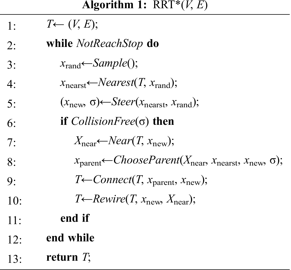
Sample: The Sample function samples a state xrand ∈ Xfree randomly.
Nearest(T, x): Given tree T and a state x ∈ Xfree, this function returns xnearest ∈ T.V, which is the closest one to x in terms of a given distance function.
Steer(x, x'): Given two states x, x' ∈ X, the Steer function steers from x to x' along a local path σ : [0,1] and returns a state xnew ∈ X such that σ(0) = x and σ(1) = xnew.
CollisionFree(x, x'): Given two states x, x' ∈ X, the Boolean CollisionFree function returns true if the path σ : [0,1] → Xfree such that σ(0) = x and σ(1) = xnew. If the CollisionFree function returns true, the new vertex and edge will be added to the tree.
NotReachStop: Returns true if the stop criteria for iterating or the goal point is not reached.
Note that the Nearest function returns all the vertices in the hypersphere with a specific radius centered at xnew which are used in the ChooseParent function.
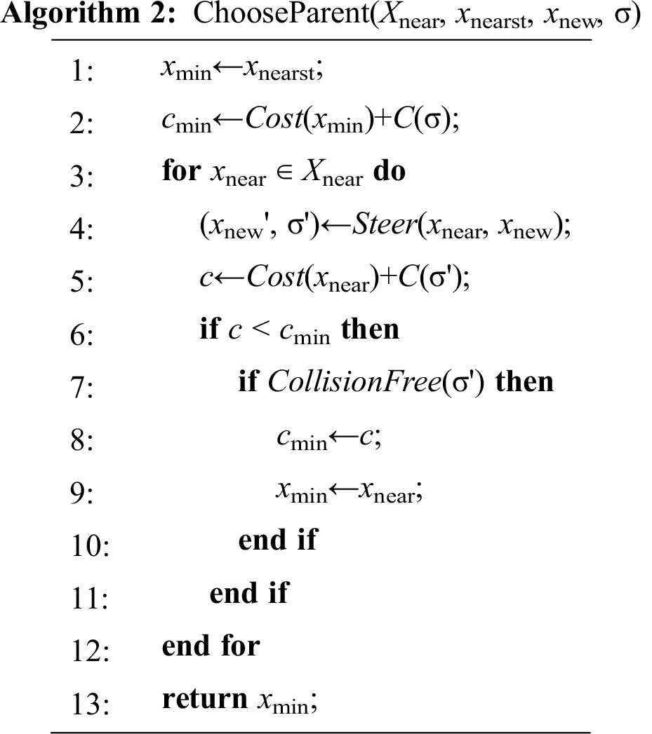
There are two optimization procedures in RRT*: ChooseParent and Rewire. The pseudo-codes of ChooseParent and Rewire are presented in Algorithm 2 and Algorithm 3, respectively. The ChooseParent function searches the vertices in the neighborhood of xnew to find a vertex that can get to xnew with the lowest total cost.
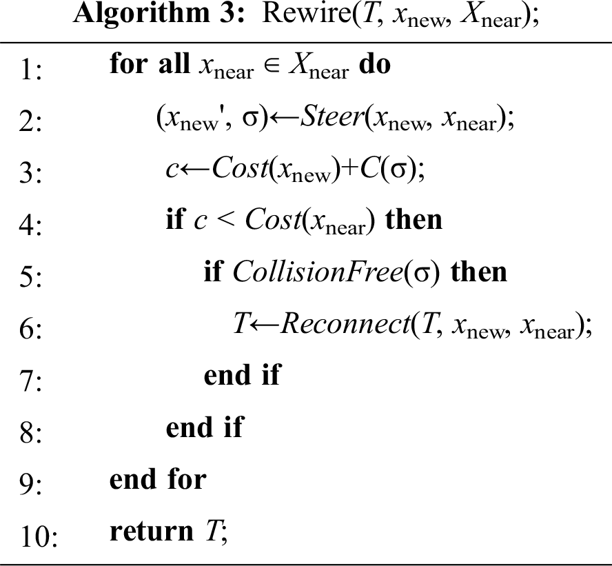
The Rewire function tries to find the vertices in the neighborhood of xnew, which can be reached by xnew with a lower cost than their current parents and rewires them.
There are two special changes in the Q-RRT* algorithm compared with RRT* as shown in Algorithm 4 and Algorithm 5. In the ChooseParent function, the parents of vertices in the neighborhood of xnew are also considered (Lines 8 and 9, Algorithm 4). The optimization efficiency can be improved by expanding the search scope. However, it does not increase the computation time too much since the vertices in Xnear usually have the same parent.
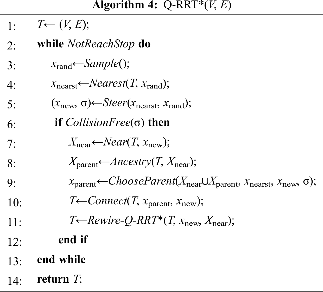
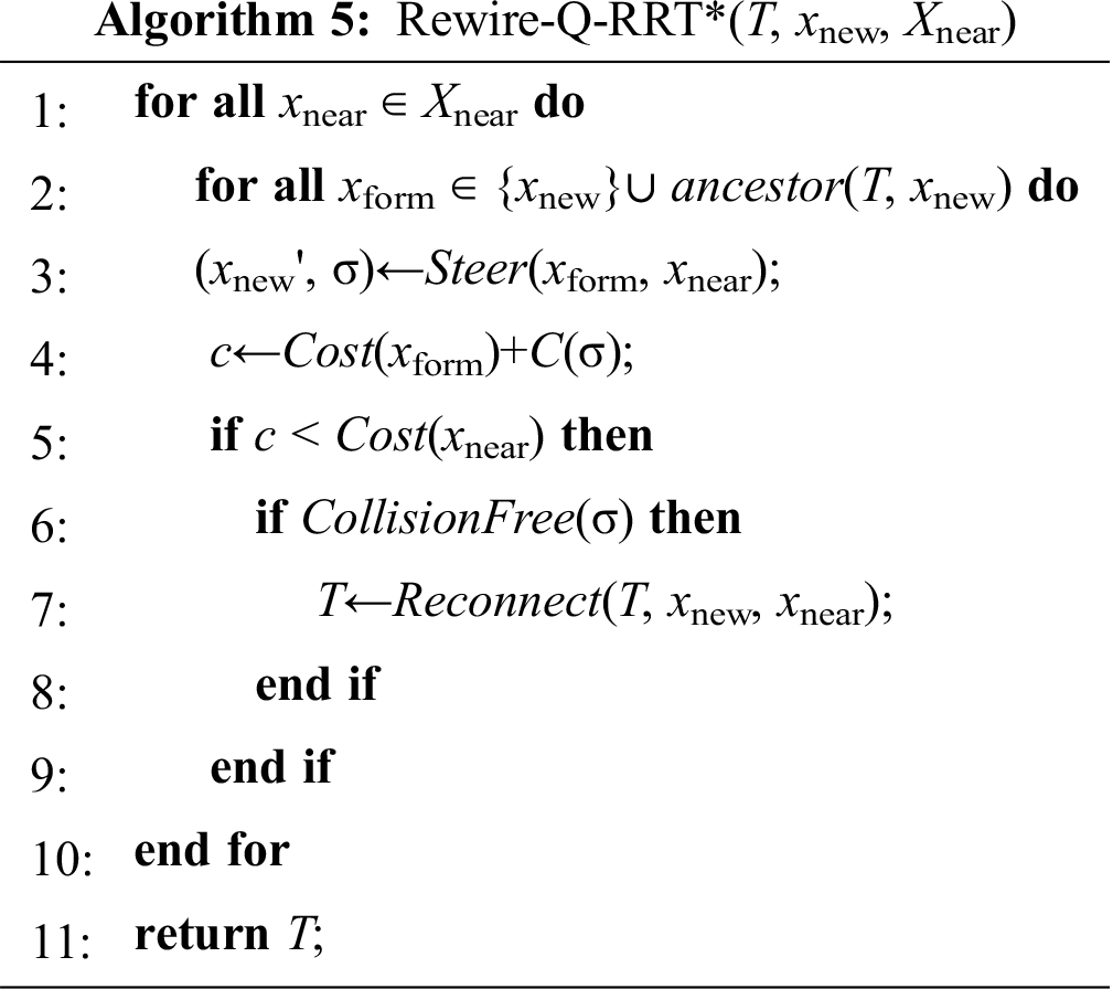
In the Rewire function, the parents of xnew are considered to further improve the optimization efficiency (Line 2, Algorithm 5). The two main new functions in Q-RRT* are as follows:
ancestor: Given a graph G = (V, E), a vertex x, and a natural number d ∈ ℕ, it returns the dth parent of x.
Ancestry: Given a graph G = (V, E) and a vertex x, it returns Ø if d = 0; otherwise, it returns
Earlier work [18] proposed an improved A* algorithm based on virtual light, which is called LA*. In the LA* algorithm, a virtual light is set up at xgoal. The virtual light lights up the map according to the characteristics of light propagation along a straight-line. The areas where light cannot reach are marked as dark. The light intensity is the strongest at xstart and decreases as the propagation distance of the light becomes longer. Thus the light intensity can be regarded as a kind of heuristic information on the map. The planner can search for areas with higher light intensity. This kind of phototaxis mechanism can greatly speed up finding the solution.
The beam spreads from the virtual light just like the beam spreads from a flashlight. The direction of the beam is towards xstart, and the beam angle is less than or equal to 180°. The beam starts from xgoal, and each vertex that is illuminated by the beam has a light intensity noted by BRIGHT as shown in Fig. 1a. As the BRIGHT value increases, the light intensity decreases in the actual program, which facilitates processing. Therefore, the BRIGHT value of xgoal is 0.
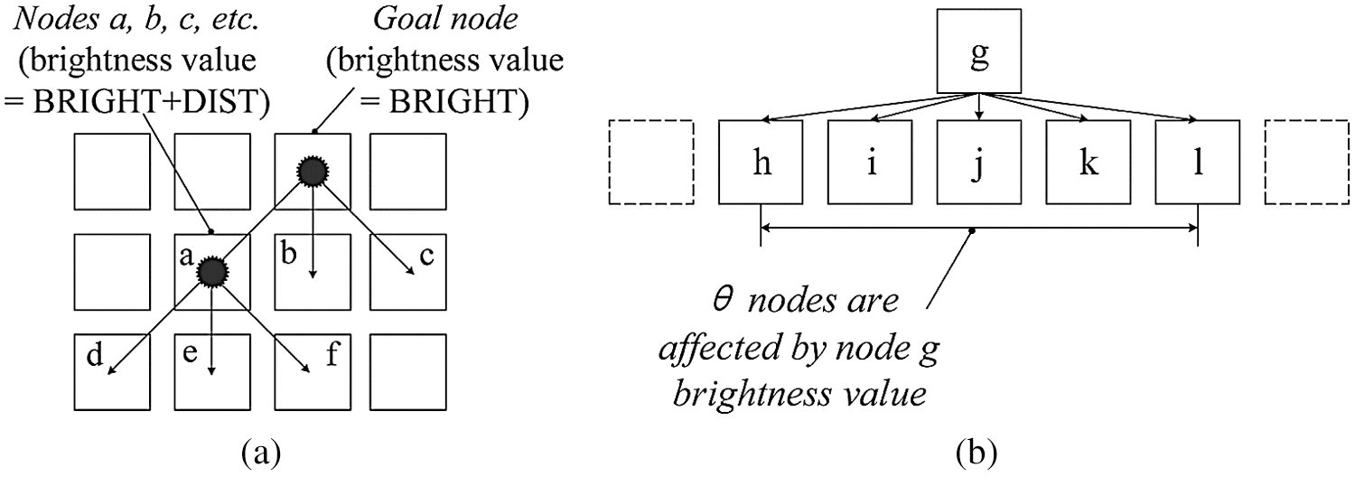
Figure 1: Diagram of the light propagation mechanism (a) 90° light beam pattern (θ = 3) (b) The generalized light beam angle pattern (any θ)
xgoal is set up at the top-middle position of the map as shown in Fig. 2b. The lighted map is represented by a grayscale image, and the light regions have a small BRIGHT value, while the dark regions have a high BRIGHT value. In the following description, the lighted map is noted by LMap for convenience. The number of successor affected vertices is given by θ (θ is an odd number). The case of when θ is 3 is shown in Fig. 1a. The successor-affected vertices of vertex a are d, e, and f. The BRIGHT value of the three vertices is equal to the BRIGHT value of a plus the distance from vertex a to each vertex. The unaffected vertices are marked DARK, which is a very large value. If a vertex is affected by multiple predecessor vertices, its BRIGHT value is set to be the minimum value, which means that the light travels along the shortest path.
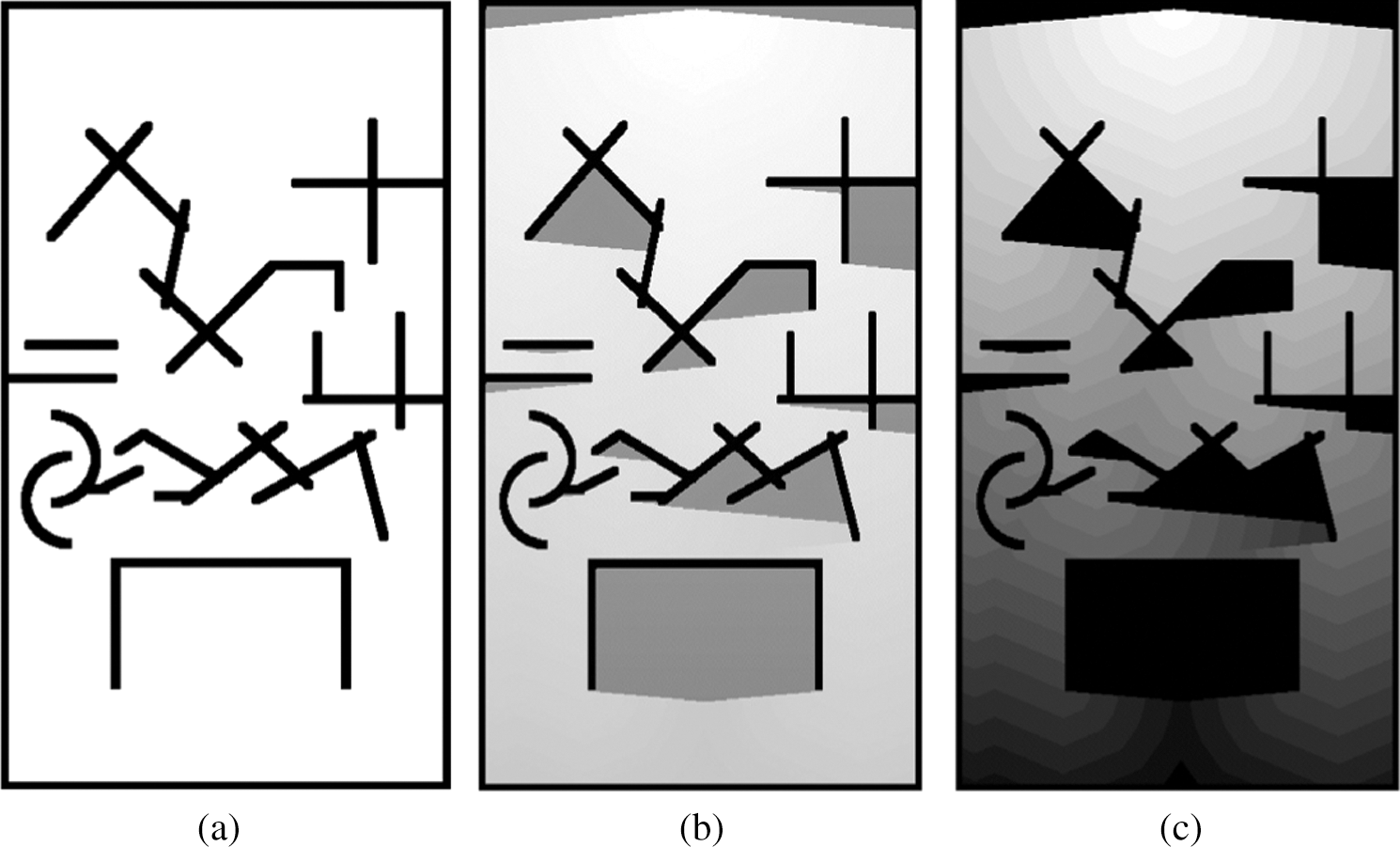
Figure 2: Maps under different representations (a) Original map (b) Lighted map (c) Contour map
The beam angle is determined by θ, θ ∈[3, max(w, h)], where w and h are the width and height of the map respectively. When θ is 3, the beam angle corresponds to the 90° pattern as shown in Fig. 1a. When θ is equal to max(w, h), it corresponds to the 180° pattern. The generalized light beam angle pattern is shown in Fig. 2b. If a vertex is blocked by an obstacle whose width is greater than θ and the light beam cannot reach the vertex, then the BRIGHT value of the vertex is set to be DARK.
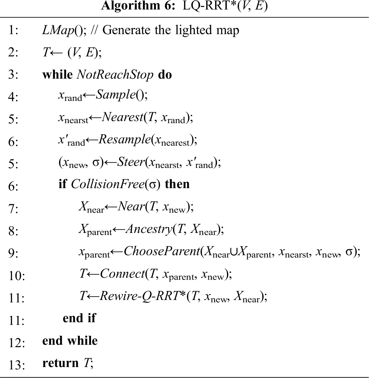
A novel algorithm called LQ-RRT* is proposed in this paper. The pseudo-code of LQ-RRT* is presented in Algorithm 6. The LMap function generates the lighted map according to the scheme described earlier (Line 1, Algorithm 6). A contour map, where the propagation of light intensity is depicted clearly, is shown in Fig. 2c to provide a better understanding of LMap. Unlike RRT* and Q-RRT*, LQ-RRT* constructs a light intensity perception region that is a semicircle centered at xnearest. The Resample function is designed to resample n vertices in the perception region in different directions as shown in Fig. 3. Next, it returns x'rand, which has the lowest BRIGHT value in the n vertices. In the LQ-RRT* algorithm, the Sample and Nearest functions are used to determine which vertex is to be expanded, and the Resample function determines the better direction to be expanded.
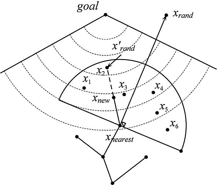
Figure 3: Diagram of Resample function
In this section, LQ-RRT* is compared with RRT* and Q-RRT* in three different environment maps as shown in Fig. 4. Map 1 is the obstacle-free scenario shown in Figs. 4a–4c. Map 2 and Map 3 are scenarios cluttered with different types of obstacles as shown in Figs. 4d–4i, respectively. The map size is 406 m × 710 m. xstart is set at the bottom of the map, and xgoal is set at the top of the map. The parameters in experiments are the depth d, resample number n, and beam angle θ. The parameters are the same in all experiments to allow a fair comparison. In the ancestor and Ancestry functions, the value of d is 1. The resample number n is 6, and the beam angle θ is 23.
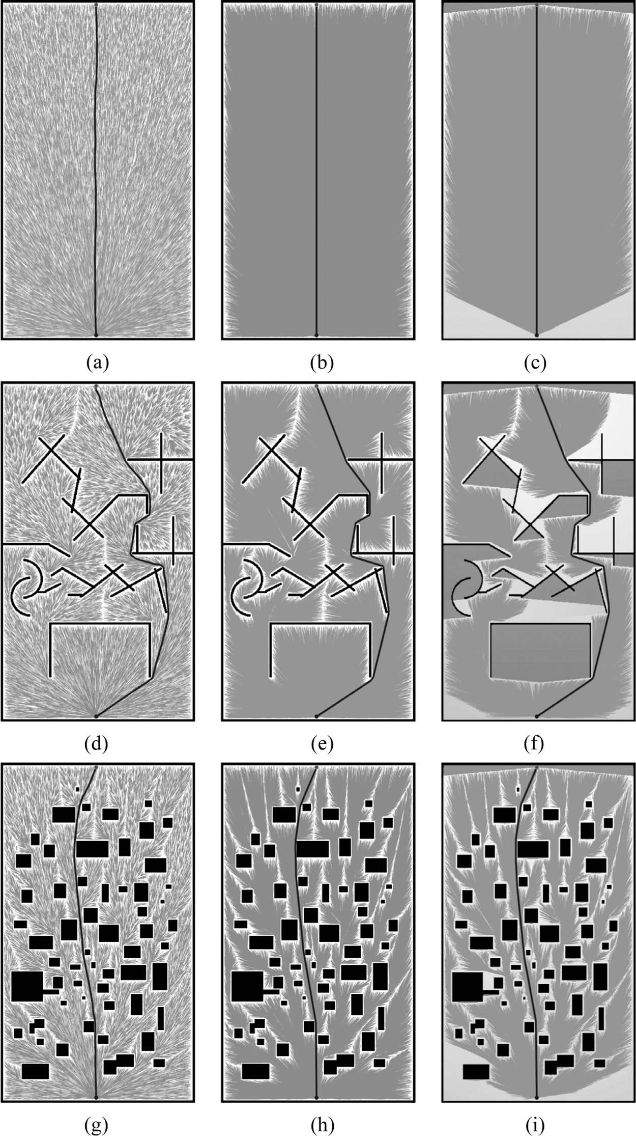
Figure 4: Generated path with 60000 samples in different maps (a) RRT* (b) Q-RRT* (c) LQ-RRT* (d) RRT* (e) Q-RRT* (f) LQ-RRT* (g) RRT* (h) Q-RRT* (i) LQ-RRT*
The final paths generated by different algorithms with 60,000 samples in the three maps are shown in Fig. 4. Although 60,000 samples have been used, the paths of RRT* are still not optimal (Fig. 4). In comparison, Q-RRT* and LQ-RRT* generate straighter paths. Meanwhile, the proposed algorithm can reduce the sample space effectively, especially when there are several areas marked with DARK on the map.
Statistical information is presented in Tabs. 1–3. Three indicators are utilized to compare the performance of the three algorithms. In Tabs. 1–3, the third and fifth columns are the length of the optimized path and the total vertices of the tree. The fourth column is the time to find a solution of 1.05*lenoptimal, where lenoptimal is the length of the optimal solution. lenoptimal of the three maps are 690 m, 851.36 m, and 699.11 m.
Table 1: Results comparison of Map 1
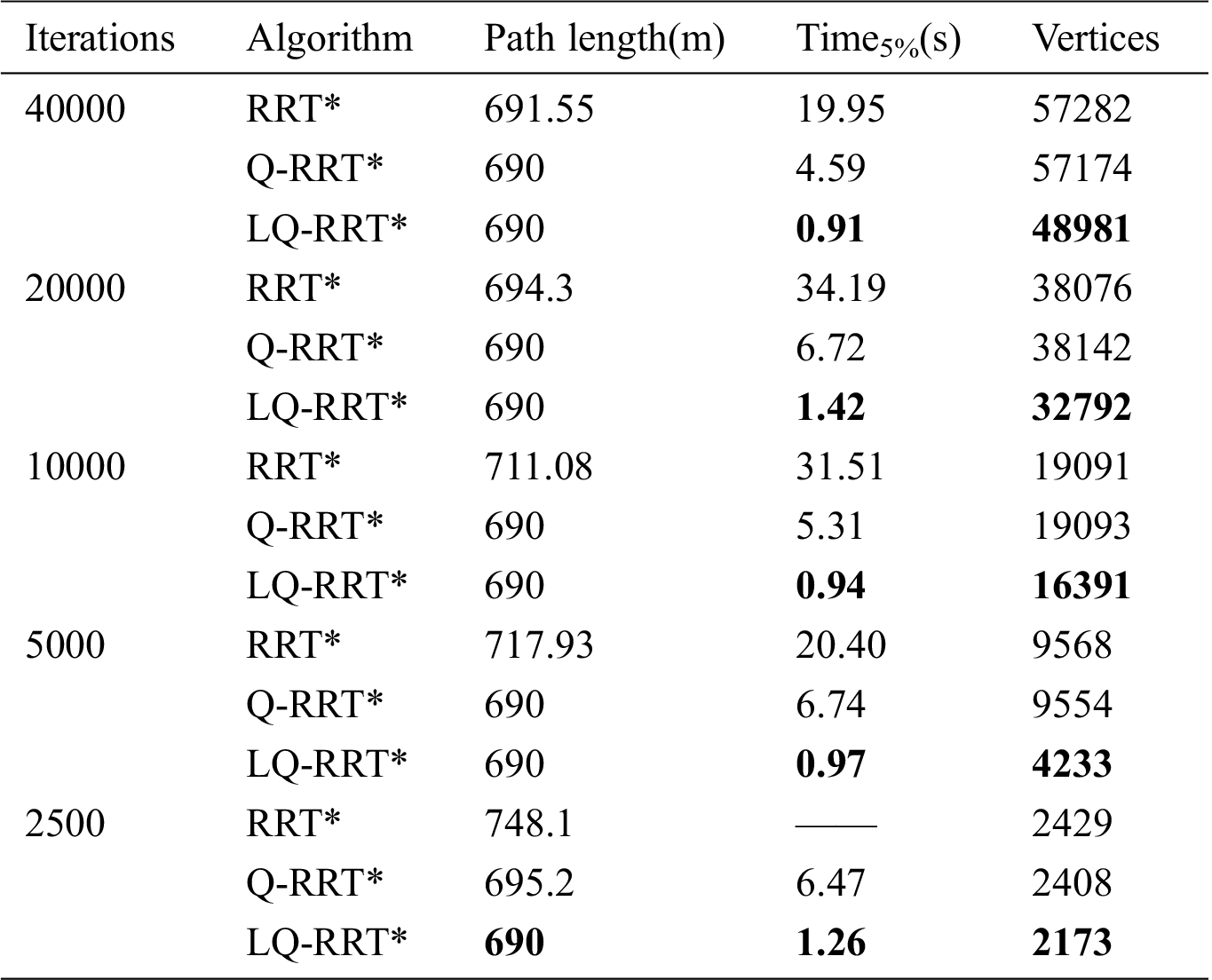
Table 2: Results comparison of Map 2
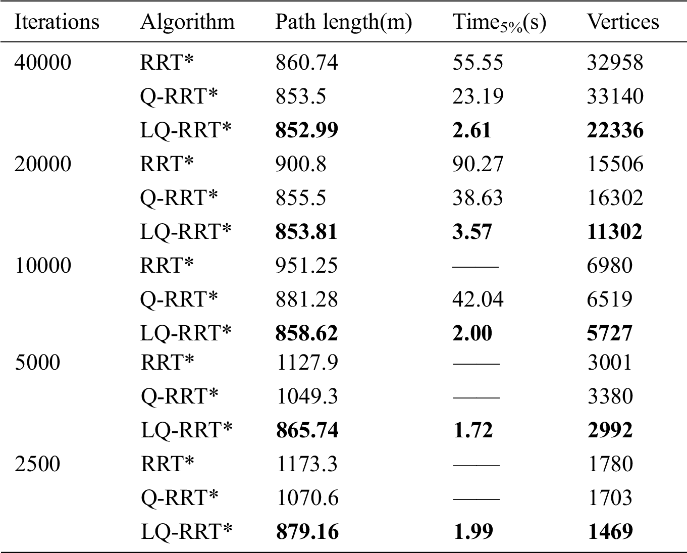
Table 3: Results comparison of Map 3
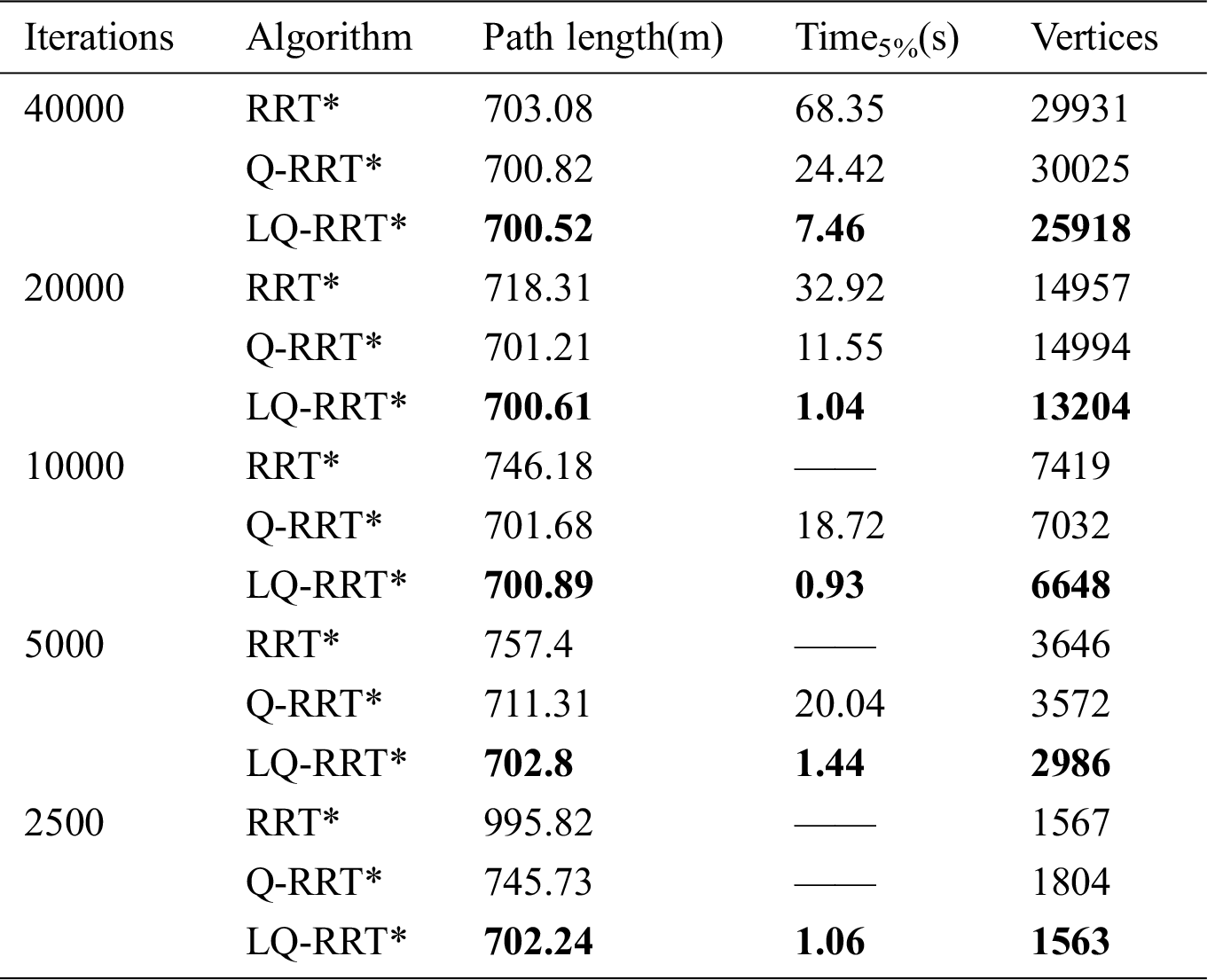
Q-RRT* and LQ-RRT* converge to the optimal solution when the number of iterations reduces from 40,000 to 5000 as shown in Tab. 1. Only the LQ-RRT* algorithm converges to the optimal solution when the number of iterations reduces to 2500. The indicator “Time5%” shows that LQ-RRT* has a faster convergence rate than the other two algorithms, and the indicator “Vertices” shows that LQ-RRT* consumes the lowest memory. The same conclusions can be obtained for the two indicators from Tabs. 2 and 3.
LQ-RRT* generates the shortest path in all experiments as shown in Tabs. 2 and 3. The path lengths of RRT* and Q-RRT* gradually increase when the total number of iterations decreases. Meanwhile, although the path length of LQ-RRT* also increases, it is still asymptotically optimal. RRT* and Q-RRT* cannot find a solution with path length less than lenoptimal when the number of iterations is small.
RRT* is an optimization algorithm. However, its main disadvantage is that the convergence rate is too low. An improved Q-RRT* algorithm, which we call LQ-RRT*, is proposed in this paper to overcome this problem. In Q-RRT*, ChooseParent and Rewire functions are modified to speed up the convergence. The concept of virtual light is introduced in this paper. Virtual light works like a flashlight. It lights up the map by light beam propagation and generates heuristic information on the map. Q-RRT* combined with the heuristic information can further accelerate the convergence of the solution. The results of experiments show that LQ-RRT* is quicker and consumes less memory than RRT* and Q-RRT*. In future work, it will be necessary to test the performance of LQ-RRT* in a dynamic environment.
Acknowledgement: The authors would like to thank the Jiangsu Electronic Data Forensics Analysis and Research Center (No. 2019SJPT002) and the Key Laboratory of Digital Forensics of Jiangsu Public Security Department. We also thank LetPub (www.letpub.com) for its linguistic assistance during the preparation of this manuscript.
Funding Statement: This work was supported by the Natural Science Foundation of the Jiangsu Higher Education Institutions of China [grant number 19KJB510022] and the Startup Research Foundation for Advanced Talents [grant number JSPIGKZ/2911119220].
Conflicts of Interest: The authors declare that they have no conflicts of interest to report regarding the present study.
1. Z. Chen, D. Wang, G. Chen, Y. Ren and D. Du, “A hybrid path planning method based on articulated vehicle model,” Computers, Materials & Continua, vol. 65, no. 2, pp. 1781–1793, 2020. [Google Scholar]
2. N. Lin, J. Tang, X. Li and L. Zhao, “A novel improved bat algorithm in UAV path planning,” Computers Materials & Continua, vol. 61, no. 1, pp. 323–344, 2019. [Google Scholar]
3. V. Mezhuyev, Y. Gunchenko, S. Shvorov and D. Chyrchenko, “A method for planning the routes of harvesting equipment,” Intelligent Automation & Soft Computing, vol. 26, no. 1, pp. 121–132, 2020. [Google Scholar]
4. D. Wu, Y. Liu, Z. Xu and W. Shang, “Design and development of unmanned surface vehicle for meteorological monitoring,” Intelligent Automation & Soft Computing, vol. 26, no. 5, pp. 1123–1138, 2020. [Google Scholar]
5. J. Wang, T. Zhang, B. Jin and S. Wu, “A novel sins/iusbl integration navigation strategy for underwater vehicles,” Journal of Cyber security, vol. 1, no. 1, pp. 1–10, 2019. [Google Scholar]
6. P. E. Hart, N. J. Nilsson and B. Raphael, “A formal basis for the heuristic determination of minimum cost paths,” IEEE Transactions on Systems Science and Cybernetics, vol. 4, no. 2, pp. 100–107, 1968. [Google Scholar]
7. A. Stentz, “Optimal and efficient path planning for partially known environments,” in Proc. ICRA, San Diego, CA, USA, pp. 3310–3317, 1994. [Google Scholar]
8. K. Daniel, A. Nash, S. Koenig and A. Felner, “Theta*: Any-angle path planning on grids,” Journal of Artificial Intelligence Research, vol. 39, pp. 533–579, 2010. [Google Scholar]
9. S. M. LaValle, “Rapidly-exploring random trees: A new tool for path planning,” in Technical Report, Ames, Iowa, USA: Iowa State University, No. 98-11, 1998. [Google Scholar]
10. J. J. Kuffner and S. M. LaValle, “RRT-connect: An efficient approach to single-query path planning,” in Proc. ICRA, San Francisco, CA, USA, 2, pp. 995–1001, 2000. [Google Scholar]
11. C. Urmson and R. Simmons, “Approaches for heuristically biasing RRT growth,” in Proc. IROS, Las Vegas, NV, USA, 2, pp. 1178–1183, 2003. [Google Scholar]
12. D. Ferguson and A. Stentz, “Anytime RRTs,” in Proc. IROS, Beijing, China, pp. 5369–5375, 2006. [Google Scholar]
13. Q. D. Zhu, Y. B. Wu, G. Q. Wu and X. Wang, “An improved anytime RRTs algorithm,” in Proc. Artificial Intelligence and Computational Intelligence, Shanghai, China, pp. 268–272, 2009. [Google Scholar]
14. S. Karaman and E. Frazzoli, “Sampling-based algorithms for optimal motion planning,” The International Journal of Robotics Research, vol. 30, no. 7, pp. 846–894, 2011. [Google Scholar]
15. F. Islam, J. Nasir, U. Malik, Y. Ayaz and O. Hasan, “RRT*-smart: Rapid convergence implementation of RRT* towards optimal solution,” in Proc. Mechatronics and Automation, Chengdu, China, pp. 1651–1656, 2012. [Google Scholar]
16. J. D. Gammell, S. S. Srinivasa and T. D. Barfoot, “Informed RRT*: Optimal sampling-based path planning focused via direct sampling of an admissible ellipsoidal heuristic,” in Proc. IROS, Chicago, IL, USA, pp. 2997–3004, 2014. [Google Scholar]
17. I. B. Jeong, S. J. Lee and J. H. Kim, “Quick-RRT*: Triangular inequality-based implementation of RRT* with improved initial solution and convergence rate,” Expert Systems with Applications, vol. 123, no. 2, pp. 82–90, 2019. [Google Scholar]
18. M. Hawa, “Light-assisted A⁎ path planning,” Engineering Applications of Artificial Intelligence, vol. 26, no. 2, pp. 888–898, 2013. [Google Scholar]
 | This work is licensed under a Creative Commons Attribution 4.0 International License, which permits unrestricted use, distribution, and reproduction in any medium, provided the original work is properly cited. |