Computer Systems Science & Engineering DOI:10.32604/csse.2021.014909
Article

Extended Rama Distribution: Properties and Applications

Khaldoon M. Alhyasat1,*, Kamarulzaman Ibrahim1, Amer Al-Omari2 and Mohd Aftar Abu Bakar1

1Department of Mathematical Sciences, Faculty of Science and Technology, Universiti Kebangsaan Malaysia, 43600 UKM, Bangi, Selangor, Malaysia
2Department of Mathematics, Faculty of Science, Al al-Bayt University, Mafraq, Jordan
*Corresponding Author: Khaldoon M. Alhyasat. Email: p105764@siswa.ukm.edu.my
Received: 26 October 2020; Accepted: 05 February 2021

Abstract: In this paper, the Rama distribution (RD) is considered, and a new model called extended Rama distribution (ERD) is suggested. The new model involves the sum of two independent Rama distributed random variables. The probability density function (pdf) and cumulative distribution function (cdf) are obtained and analyzed. It is found that the new model is skewed to the right. Several mathematical and statistical properties are derived and proved. The properties studied include moments, coefficient of variation, coefficient of skewness, coefficient of kurtosis and moment generating function. Some simulations are undertaken to illustrate the behavior of these properties. In addition, the reliability analysis of the distribution is investigated through the hazard rate function, reversed hazard rate function and odds function. The parameter of the distribution is estimated based on the maximum likelihood method. The distributions of order statistics for ERD are also presented. The performance of the suggested model is compared with several other lifetime distributions based on some goodness of fit tests on a real dataset. It turns out that the suggested model is more flexible than its competitors considered in this study, for modeling real lifetime data.

Keywords: Coefficient of kurtosis; coefficient of skewness; order statistics; two independent Rama random variables; Maximum likelihood estimation; Rama distribution

1  Introduction

Recently, some studies on the distribution of sum of random variables have acquired some significant importance in various branches of science for fitting real data. Many authors have studied the distribution of the sum of random variables and their applications based on various base distributions, to suggest new flexible distributions. As an example, [1] suggested a power length-biased Suja distribution, whereas [2] derived the distribution for the sums of uniformly distributed random variables. Moreover, [3] introduced the distribution of the sum of mixed independent random variables pertaining to special functions. Also, [4] proposed the sum and difference of two squared correlated Nakagami variates which are in connection with the McKay distribution. In contrast, the sum of t and Gaussian random variables is suggested by [5], while [6] proposed the sum of independent gamma random variables. Reference [7] studied the sum of independent gamma random variables, while generalizations of two-sided power distributions and their convolution are introduced by [8]. Besides, [9] derived the distribution of the mixed sum of independent random variables where one of them is associated with the H-function. On the other hand, [10] obtained the distribution of the sum of mixed independent random variables pertaining to certain special functions, while [11] proposed the weighted Suja distribution and its applications in engineering. Moreover, [12] suggested a Darna distribution as a mixture of exponential and gamma distributions. Reference [13] proposed a power size biased two-parameter Akash distribution, and [14] suggested a generalization of the new Weibull-Pareto distribution. In 2019, [15] introduced a transmuted Ishita distribution and [16] proposed a Marshall-Olkin length-biased exponential distribution.

In this paper, we modified the Rama distribution, which was firstly suggested by [17], while considering the sum of two independent variables in order to propose a new lifetime distribution, named extended Rama distribution. The probability density function (pdf) of the Rama distribution is given by

f(x;θ)=θ4θ3+6(1+x3)e−θx,x>0,θ>0, (1)

and the corresponding cumulative distribution function (cdf) is given by

F(x;θ)=1−(1+θ3x3+3θ2x2+6θxθ3+6)e−θx;x>0,θ>0. (2)

The rest of the paper is organized as follows. In Section 2, the new distribution is presented in terms of its functions and shapes. Some statistical properties are given in Section 3, while in Section 4, the parameter of the distribution is estimated using the maximum likelihood method. Distributions of order statistics based on samples selected from ERD are presented in Section 5. Moreover, the reliability analysis based on ERD is given in Section 6. An application using a real data set is provided in Section 7. Finally, the paper is concluded in Section 8.

1.1 The New Model

Let X and Y be two independent random variables defined on the interval [0,∞) follows the Rama density with parameter θ . Suppose that the density of the random variable Z=X+Y indicates the distribution of interest, and fX,fY and fZ denote the densities for random variables X, Y and Z, respectively. Therefore,

fX(x)=fY(x)=θ4θ3+6(1+x3)e−θx,x>0,θ>0, (3)

and

fZ(x)=∫0∞f(x−t).f(t)dt. (4)

Hence, a random variable X is said to follow the ERD if its pdf is given by

f(x;θ)=θ8(6+θ3)2(x+x42+x7140)e−θx,x>0,θ>0. (5)

It is easy to show and validate Eq. (5) as follows:

It is of interest to note here that

Theorem 1: Let X be a random variable follows the ERD with parameter θ. The cumulative distribution function of X is defined as

F(x;θ)=1−(x2θ2[42x3θ3+7x4θ4+x5θ5+(3+θ3)(840+280xθ+70x2θ2)]140(6+θ3)2+1+xθ)e−xθ. (6)

Proof: The cdf of the ERD can be derived as follows:

To study the behavior of the ERD, we consider x ∈ (0, 2]. In Fig. 1, the plots of the pdf and cdf of the ERD for various values of the parameter of the distribution are presented.

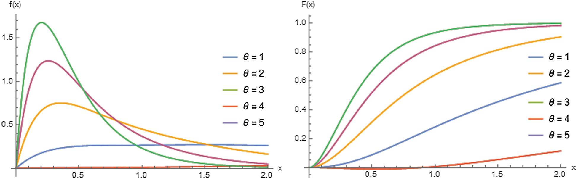
Figure 1: The pdf and cdf of ERD for θ = 1, 2, 3, 4, 5

Referring to Fig. 1, it is clear that ERD is asymmetric and skewed to the right over the interval (0, 2]. The degree of the skewness depends on the parameter value.

2  Some Properties of ERD

This section presents the rth moment, mean, variance, coefficient of variation, coefficient of skewness and coefficient of kurtosis for the ERD. Some numerical calculations for these properties are also provided.

2.1 Moments

Theorem 2: Let X∼f(x;θ) . Then, the rth moment of X is given by

E(Xr)=θ−r(70θ3(2θ3Γ(r+2)+Γ(r+5))+Γ(r+8))140(θ3+6)2,θ>0;r=1,2,3,... (7)

Proof: The rth moment of the ERD can be obtained by

Based on Eq.7, we can obtain the first four moments of the ERD as

μ1′=48+2θ36θ+θ4,μ2′=6432+60θ3+θ6θ26+θ32,μ3′=241080+105θ3+θ6θ36+θ32 and μ4′=1202376+168θ3+θ6θ46+θ32, (8)

respectively. Therefore, the variance of the ERD is

σ2=2(θ6+84θ3+144)θ2(θ3+6)2. (9)

2.2 The Coefficient of Skewness

The coefficient of skewness determines the degree of skewness of a distribution and for the ERD it is given by

Sk=μ3′−3μ1′σ2−(μ1′)3σ3=2(θ9+198θ6+324θ3+864)θ3(θ3+6)3(θ6+84θ3+144θ2(θ3+6)2)3/2. (10)

2.3 The Coefficient of Kurtosis

The coefficient of variation of the ERD is defined as

ku=μ4−4μ1μ3+6μ12σ2+3μ14σ4=6(θ3+6)2(θ6+264θ3+360)(θ6+84θ3+144)2. (11)

2.4 The Coefficient of Variation

The coefficient of variation of the ERD is defined as

Cv=σμ=θ6+84θ3+1442(θ3+24). (12)

To investigate the behavior of these measures, we calculate the values of μ,σ,Cv,Sk and Ku for the ERD for various values of θ . The results are presented in Tab. 1.

Table 1: The values of μ,σ,Cv,Sk and Ku for the ERD for different values of θ

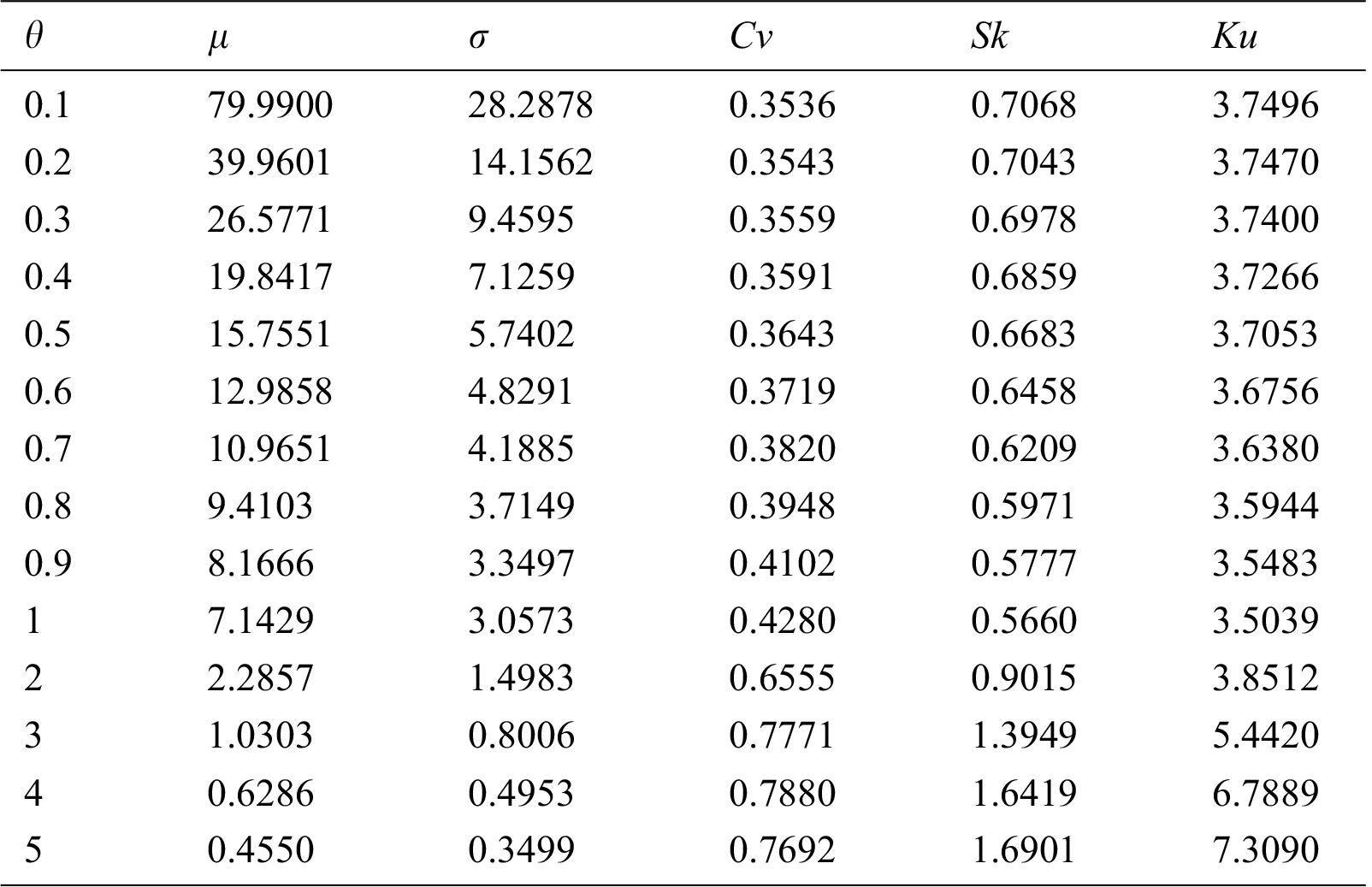
Based on Tab. 1, it can be deduced that:

1.   As the values of θ are increasing, the values of mean and standard deviation are decreasing.

2.   As the values of θ are increasing, the values of the coefficient of variation are increasing.

3.   The coefficient of skewness and coefficient of kurtosis are decreasing as the values of theta are increasing up to θ=1 , then start increasing.

Theorem 3: The moment generating function of the ERD is given by

E(etx)=θ8(θ3−t3+3θt2−3θ2t+6)2(θ3+6)2(t−θ)8. (13)

Proof: The moment generating function can be derived as follows

3  Maximum Likelihood Estimation

Let X1,X2,...,Xn be a random sample of size n chosen from the ERD with parameter θ . The maximum likelihood estimator for the ERD parameter can be derived as follows. The likelihood function of θ is given by

L(θ)=∏i=1nθ8(6+θ3)2(xi+xi42+xi7140)e−θxi=(θ8(6+θ3)2)n∏i=1n(xi+xi42+xi7140)e−θxi=θ8n(6+θ3)2ne∑i=1n−θxi∏i=1n(xi+xi42+xi7140)=θ8n(6+θ3)2ne−nθx¯∏i=1n(xi+xi42+xi7140) .

Then, the log-likelihood function is

lnL(θ)=ln[θ8n(6+θ3)2ne−nθx¯∏i=1n(xi+xi42+xi7140)]=8nln(θ)−2nln(6+θ3)−nθx¯+∑i=1nln(xi+xi42+xi7140). (14)

By taking the first derivative of Eq.14 with respect to θ and setting the results to 0, we obtain

∂lnL(θ)∂θ=8nθ−6nθ2θ3+6−nx¯=0. (15)

Since there is no closed form solution for Eq. 15, i.e. the MLE of θ , denoted as θ^ , is the numerical solution for this equation.

4  Order Statistics

Assume that X1,X2,...Xn denote a random sample of size n from the ERD distribution. Also, suppose that X(1:n),X(2:n),...,X(n:n) denote the corresponding order statistics of the sample. The density function of the ith order statistic X(i:n) for 1≤i≤n is given by

f(i:n)(x)=n!(i−1)!(n−i)![F(x)]i−1[1−F(x)]n−if(x). (16)

By substituting the pdf and cdf of the ERD in Eq. (16), the pdf of X(i:n) is

f(i:n)(x,θ)={n!θ8(x7140+x42+x)(1−(θ2x2(θ5x5+7θ4x4+42θ3x3+(θ3+3)(θ+70θ2x2+1120))140(θ3+6)2+θx+1)e−θx)i−1((θ2x2(θ5x5+7θ4x4+42θ3x3+(θ3+3)(θ+70θ2x2+1120))140(θ3+6)2+θx+1)e−θx)n−i}(θ3+6)2(i−1)!(m−i)!e−θx. (17)

From Eq. (17), the pdfs of the smallest order statistic X(1:n) and the largest order statistic X(n:n) are, respectively be given by

f(1:n)(x;θ)=n!θ8(x7140+x42+x)(θ2x2(θ5x5+7θ4x4+42θ3x3+(θ3+3)(θ+70θ2x2+1120))140(θ3+6)2+θx+1)n−1(θ3+6)2(n−1)!e−θnx, (18)

and

f(n:n)(x;θ)=n!θ8(x7140+x42+x)(1−e−θx(θ2x2(θ5x5+7θ4x4+42θ3x3+(θ3+3)(θ+70θ2x2+1120))140(θ3+6)2+θx+1))n−1(θ3+6)2(n−1)!e−θx. (19)

5  Reliability Analysis

This section defines the reliability (survival) function, hazard rate function, reversed hazard rate function and odd function for the suggested model. The reliability function of the ERD is given by

R(x;θ)=1−F(x;θ)=(θ2x2(θ5x5+7θ4x4+42θ3x3+(θ3+3)(θ+70θ2x2+840+280))140(θ3+6)2+(θx+1))e−θx. (20)

On the other hand, the hazard rate function of the ERD is given by

H(x;θ)=f(x;θ)1−F(x;θ)=θ8(x7140+x42+x)(θ3+6)2(θ2x2(θ5x5+7θ4x4+42θ3x3+(θ3+3)(θ+70θ2x2+1120))140(θ3+6)2+θx+1). (21)

Meanwhile, the reversed hazard rate function for the ERD distribution is defined as

RH(x;θ)=f(x;θ)F(x;θ)=θ8(x7140+x42+x)e−θx(θ3+6)2(1−e−θx(θ2x2(θ5x5+7θ4x4+42θ3x3+(θ3+3)(θ+70θ2x2+1120))140(θ3+6)2+θx+1)). (22)

The odds function for ERD is defined as

O(x;θ)=F(x;θ)1−F(x;θ)=eθxθ2x2(θ5x5+7θ4x4+42θ3x3+(θ3+3)(θ+70θ2x2+1120))140(θ3+6)2+θx+1−1. (23)

Figs. 2–4 reveal that the reliability and reversed hazard rate functions decrease as the values of x increase. In contrast, the hazard and odd functions are increasing with x for various values of the parameter θ.

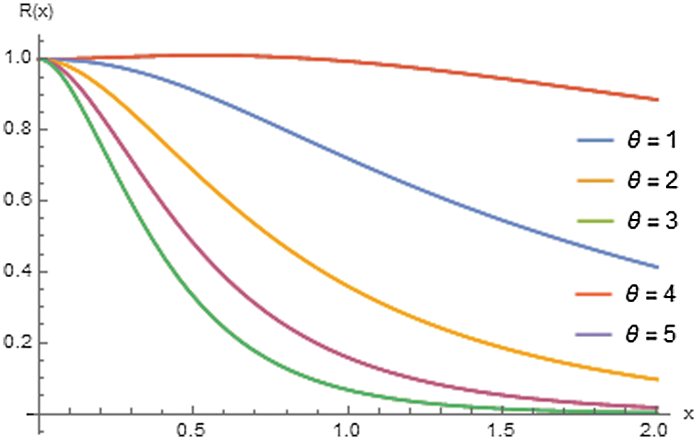
Figure 2: Reliability plots of the ERD for θ =1, 2, 3, 4, 5

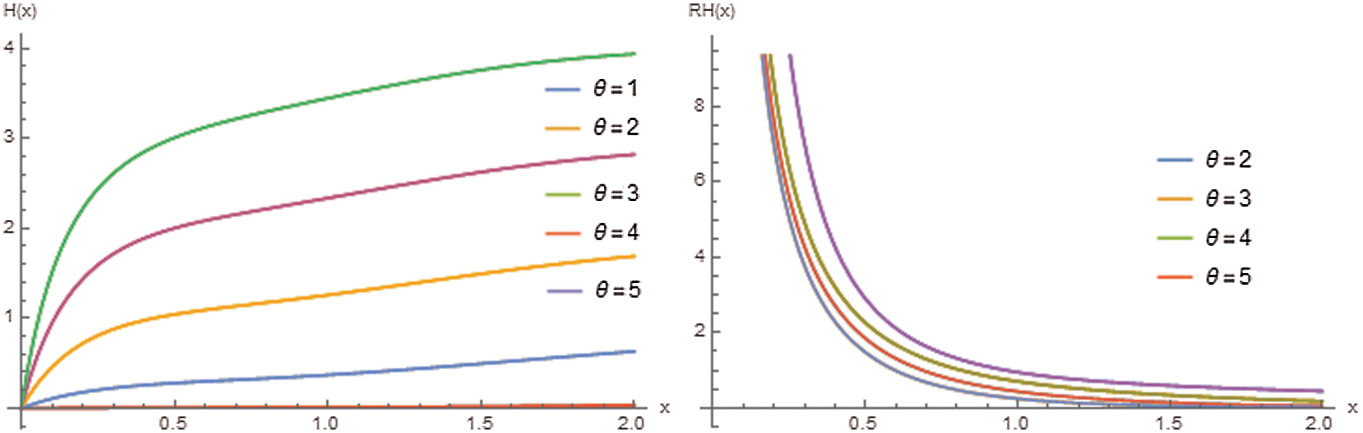
Figure 3: Plots of hazard and reversed hazard rate functions of the ERD for different values of θ

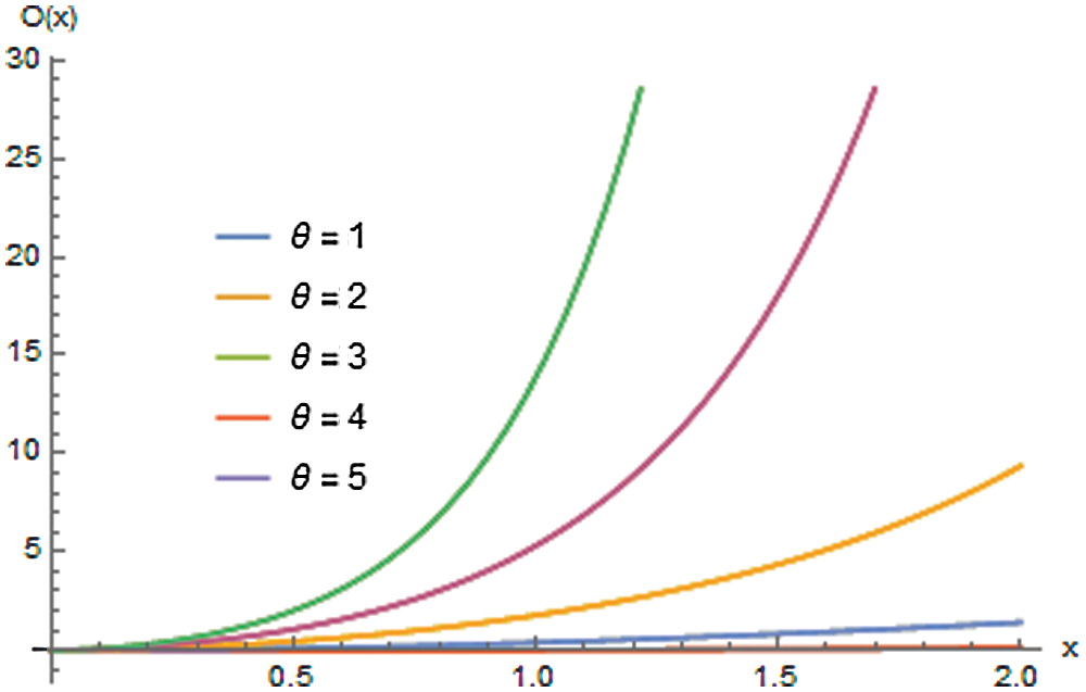
Figure 4: The plots of odds function of ERD for θ =1, 2, 3, 4, 5

6  Practical Illustration

This section compares the performance of ERD with Rama distribution, exponential distribution, Rani distribution and Maxwell length-biased distribution for fitting a real data set. The probability density functions for these distributions are as follows:

a) Rama distribution (RD) [17]:

f(x;θ)=θ4θ3+6(1+x3)e−θx,x>0,θ>0. (24)

b) Exponential distribution (ED):

f(x;λ)=λe−λx,λ>0. (25)

c) Rani distribution (RND) [18]:

f(x;θ)=θ5θ5+24(θ+x4)e−θx,θ>0. (26)

d) Maxwell length-biased distribution (MLBD) [19]:

f(x;α)=x32α4e−x22α2,x>0,α>0. (27)

The dataset explains the strength of the aircraft window glass as recorded by [20], which is given as follows:

Data: 18.83, 20.80, 21.657, 23.03, 23.23, 24.05, 24.321, 25.50, 25.52, 25.80, 26.69, 26.77, 26.78,27.05, 27.67, 29.90, 31.11, 33.20, 33.73, 33.76, 33.89, 34.76, 35.75, 35.91, 36.98, 37.08,37.09, 39.58, 44.045, 45.29, 45.381.

For comparison, we consider the Akaike Information Criterion (AIC), consistent Akaike information criterion (CAIC), Bayesian information criterion (BIC), Hannan-Quinn information criterion (HQIC) and Kolmogorov-Smirnov (KS) test statistics for measuring the goodness of fit (GOF) of the different models to the data. Parameters of the models are estimated using maximum likelihood. These (GOF) measures are defined as follows:

where φ is the number of parameters and n is the sample size. The Kolmogorov-Smirnov (KS) test is defined as KS=Supn|Fn(x)−F(x)| , where Fn(x)=1n∑i=1nIxi≤x is the empirical distribution function and F(x) is the cumulative distribution function. Generally, the smallest value of these particular measures indicates the respective model best fits the data. For assessing the goodness of fit for all the models considered, the measures are computed and the results are given in Tab. 2.

Table 2: The MLE, AIC, CAIC, BIC, HQIC and the p-value for modelling the data

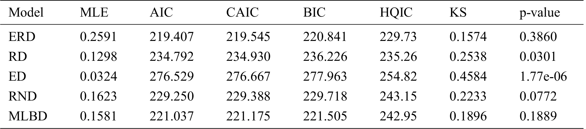
Based on Fig. 5, we notice that ERD provides the best fit for modelling the dataset. The p-value of the KS test is 0.39 which is greater than the 0.05 level of significance, indicating that ERD model is adequate for the data. In addition, the other measures of goodness of fit are found the smallest for the ERD, with the respective larger p-values, which further support that ERD as the best model.

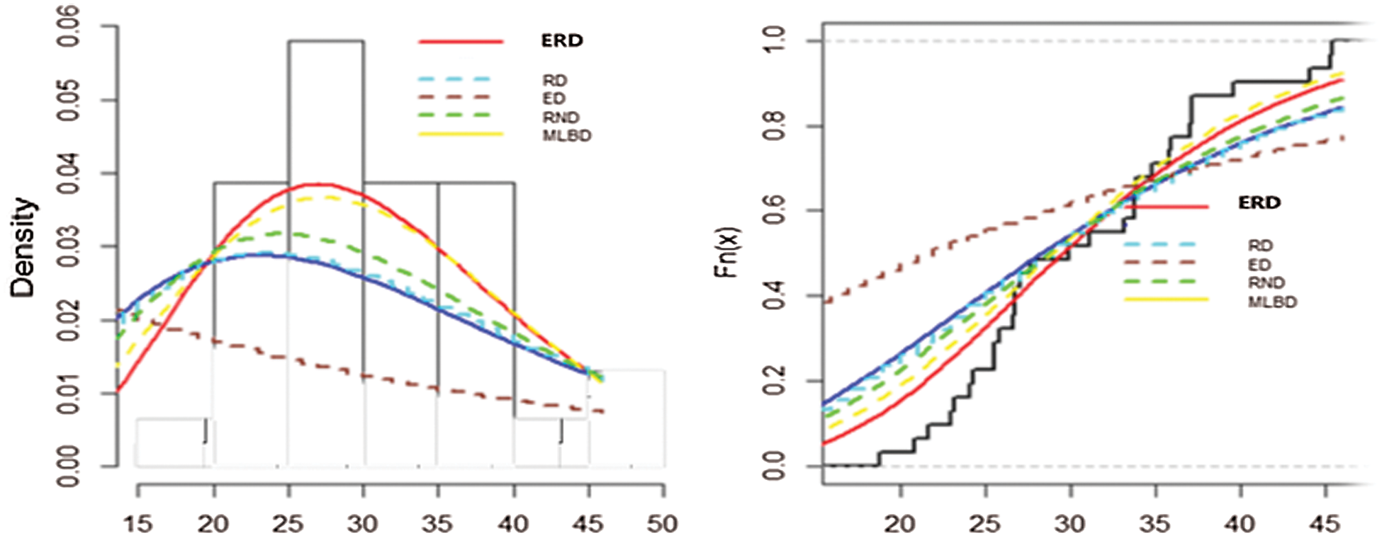
Figure 5: The histogram and empirical distribution functions of the fitted models to the data

7  Conclusions

In the present paper, an extended Rama distribution is proposed. Many mathematical and statistical properties of the new distribution are provided. The reliability, hazard rate, reversed hazard rate and odd functions of the ERD are also presented. The parameter of this distribution is obtained using MLE. In addition to a simulation study, the performance of ERD in fitting a real dataset is compared to several other models which are often used to describe the lifetime data based on several goodness of fit tests. It turns out that the ERD can be considered as a viable alternative model when modelling lifetime data. As for future work, one can estimate the parameter of the distribution using the ranked set sampling method [21–24].

Acknowledgement: The authors are sincerely grateful to the anonymous referees and the editor for their time and effort in providing constructive, and valuable comments and suggestions that have led to a substantial improvement in the paper.

Funding Statement: The authors extend their appreciation to Universiti Kebangsaan Malaysia for providing a partial funding for the work under the grant number GGPM-2017-124 and TAP-K017073 which were obtained by Mohd Aftar Abu Bakar.

Conflicts of Interest: The authors declare that they have no conflicts of interest to report the findings of the present study.

References

 1.  A. I. Al-Omari, K. M. Alhyasat, K. Ibrahim and M. A. A. Bakar, “Power length-biased Suja distribution: properties and application,” Electronic Journal of Applied Statistical Analysis, vol. 12, no. 2, pp. 429–452, 2019. [Google Scholar]

 2.  J. Albert, “Sums of uniformly distributed variables,” College Mathematics Journal, vol. 33, no. 3, pp. 201–206, 2018. [Google Scholar]

 3.  V. Chaurasia and J. Singh, “The distribution of the sum of mixed independent random variables pertaining to special functions,” International Journal of Engineering Science and Technology, vol. 2, no. 7, pp. 2601–2606, 2010. [Google Scholar]

 4.  H. Holm and M. Alouini, “Sum and difference of two squared correlated Nakagami variates in connection with the McKay distribution,” IEEE Trans. on Communications, vol. 52, no. 8, pp. 1367–1376, 2004. [Google Scholar]

 5.  G. Nason, “On the sum of and Gaussian random variables,” Statistics and Probability Letters, vol. 76, no. 12, pp. 1280–1286, 2006. [Google Scholar]

 6.  S. Provost, “On sums of independent gamma random variables,” Statistics, vol. 20, no. 4, pp. 583–591, 1989. [Google Scholar]

 7.  P. Moschopoulos, “The distribution of the sum of independent gamma random variables,” Annals of the Institute of Statistical Mathematics, vol. 37, no. 3, pp. 541–544, 1985. [Google Scholar]

 8.  J. Van Dorp and S. Kotz, “Generalisations of two-sided power distributions and their convolution,” Communications in Statistics–Theory and Methods, vol. 32, no. 9, pp. 1703–1723, 2003. [Google Scholar]

 9.  M. Gupta, “The distribution of mixed sum of independent random variables one of them associated with H – function,” Ganita Sandesh, vol. 22, no. 2, pp. 139–146, 2008. [Google Scholar]

10. V. Chaurasia and J. Singh, “The distribution of the sum of mixed independent random variables pertaining to special functions,” Int. Journal of Engineering Science and Technology, vol. 2, no. 7, pp. 2601–2606, 2010. [Google Scholar]

11. I. K. Alsmairan and I. K. A. I. Al-Omari, “Weighted Suja distribution with an application to ball bearings data,” Life Cycle Reliability and Safety Engineering, vol. 9, no. 2, pp. 195–211, 2020. [Google Scholar]

12. D. H. Shraa and A. I. Al-Omari, “Darna distribution: properties and applications,” Electronic Journal of Applied Statistical Analysis, vol. 12, no. 2, pp. 520–541, 2020. [Google Scholar]

13. K. M. Alhyasat, K. Ibrahim, A. I. Al-Omari and M. A. A. Bakar, “Power size biased two-parameter Akash distribution,” Statistics in Transition New Series, vol. 21, no. 3, pp. 73–91, 2020. [Google Scholar]

14. A. I. Al-Omari, A. Al-khazaleh and L. M. Alzoubi, “A generalization of the new Weibull-Pareto distribution,” Revista Investigacion Operacional, vol. 41, no. 1, pp. 138–146, 2020. [Google Scholar]

15. M. Garaibah and A. I. Al-Omari, “Transmuted Ishita distribution and its applications,” Journal of Statistics Applications & Probability, vol. 8, no. 2, pp. 67–81, 2019. [Google Scholar]

16. R. M. Usman, M. A. Haq, S. Hashmi and A. I. Al-Omari, “The Marshall-Olkin length-biased exponential distribution and its applications,” Journal of King Saud University-Science, vol. 31, no. 2, pp. 246–251, 2019. [Google Scholar]

17. R. Shanker, “Rama Distribution and Its Application,” Int. Journal of Statistics and Applications, vol. 7, no. 1, pp. 26–35, 2017. [Google Scholar]

18. R. Shanker, “Rani distribution and its application,” Biometrics & Biostatistics Int. Journal, vol. 6, no. 1, pp. 256–265, 2017. [Google Scholar]

19. A. Saghir, A. Khadim and Z. Lin, “The Maxwell length biased distribution: properties and estimation,” Journal of Statistical Theory and Practice, vol. 11, no. 1, pp. 26–40, 2016. [Google Scholar]

20. E. R. Fuller Jr., S.W. Freiman, J. B. Quinn, G. D. Quinn and C. Carter, “Fracture mechanics approach to the design of glass aircraft windows: a case study,” in Proc. of SPIE - The Int. Society for Optical Engineering, San Diego, CA, 2286, pp. 419-â˘A, 1994. [Google Scholar]

21. A. I. Al-Omari and C. N. Bouza, “Ratio estimators of the population mean with missing values using ranked set sampling,” Environmetrics, vol. 26, no. 2, pp. 67–76, 2015. [Google Scholar]

22. A. I. Al-Omari, “Estimation of the population median of symmetric and asymmetric distributions using double robust extreme ranked set sampling,” Revista Investigacion Operacional, vol. 31, no. 3, pp. 200–208, 2010. [Google Scholar]

23. A. A. Jemain, A. I. Al-Omari and K. Ibrahim, “Multistage median ranked set sampling for estimating the population median,” Journal of Mathematics and Statistics, vol. 3, no. 2, pp. 58–64, 2007. [Google Scholar]

24. A. A. Jemain, A. I. Al-Omari and K. Ibrahim, “Some variations of ranked set sampling,” Electronic Journal of Applied Statistical Analysis, vol. 1, no. 1, pp. 1–15, 2008. [Google Scholar]

This work is licensed under a Creative Commons Attribution 4.0 International License, which permits unrestricted use, distribution, and reproduction in any medium, provided the original work is properly cited.