DOI:10.32604/csse.2021.015030
| Computer Systems Science & Engineering DOI:10.32604/csse.2021.015030 | |
| Article |
Layout Optimization for Greenhouse WSN Based on Path Loss Analysis
1National Engineering Research Center for Information Technology in Agriculture, Beijing, 100097, China
2Beijing Research Center for Information Technology in Agriculture, Beijing Academy of Agriculture and Forestry Sciences, Beijing, 100097, China
3Key Laboratory of Agri-informatics, Ministry of Agriculture, Beijing, 100097, China
4Department of Biosystems, Mechatronics, Biostatistics and Sensors, KU Leuven, Heverlee, 3001, Belgium
*Corresponding Author: Xiao Han. Email: hxyu33@sina.com
Received: 03 November 2020; Accepted: 21 December 2020
Abstract: When wireless sensor networks (WSN) are deployed in the vegetable greenhouse with dynamic connectivity and interference environment, it is necessary to increase the node transmit power to ensure the communication quality, which leads to serious network interference. To offset the negative impact, the transmit power of other nodes must also be increased. The result is that the network becomes worse and worse, and node energy is wasted a lot. Taking into account the irregular connection range in the cucumber greenhouse WSN, we measured the transmission characteristics of wireless signals under the 2.4 Ghz operating frequency. For improving network layout in the greenhouse, a semi-empirical prediction model of signal loss is then studied based on the measured data. Compared with other models, the average relative error of this semi-empirical signal loss model is only 2.3%. Finally, by combining the improved network topology algorithm and tabu search, this paper studies a greenhouse WSN layout that can reduce path loss, save energy, and ensure communication quality. Given the limitation of node-degree constraint in traditional network layout algorithms, the improved algorithm applies the forwarding constraint to balance network energy consumption and constructs asymmetric network communication links. Experimental results show that this research can realize the energy consumption optimization of WSN layout in the greenhouse.
Keywords: Path loss model; vegetable greenhouse; network topology; network layout
The Internet of Things (IoT), as a network that connects things to things and things to people, is considered the main driving force for 5G development. Wireless sensor networks (WSN) play an important role in the basis of the IoT. Sensors in various terminal devices perform real-time monitoring and collect a large amount of information. After data collection, the networks will analyze the data and serve the upper software. It can be seen that in-depth research on WSN helps to improve IoT performance in an all-round way. Greenhouse WSN can control production factors in time and space and improve crop yield and quality [1]. Precision operation depends on the data acquisition that includes crops, climate, soil, fertilizer, water, and so on [2,3]. Many researchers have applied WSN to support vegetable disease identification, real-time control, decision-making, etc. [4–7]. In agriculture, sensors must transmit a large amount of data and usually require a long monitoring period. Due to the limited energy, frequent replacement or redeployment of nodes will not only bring about high cost, but also lose the monitoring data, and result in a failure to make control decisions timely. Besides, the communication ability can be affected by many factors (vegetable plants, etc.), which complicates network connectivity [8].
By planning the sensor location and communication path, a connected network with small path loss can be built [9], which is beneficial to reduce network energy consumption and prolong network lifetime. Cama-Pinto et al. [10] have studied the signal characteristics in a tomato greenhouse. They proposed that when the line-of-sight communication link between nodes is blocked by dense vegetation, the WSN performance could be affected due to extra signal loss. However, they did not further explain how to applied their research to optimize the greenhouse WSN. In other researches, it is generally considered that the signal is transmitted in an ideal space, ignoring the signal attenuation complexity in the actual environment. The greenhouse is closed and mostly made of steel tubes. Signal transmission in the greenhouses is quite different from that in an ideal space. Therefore, research on signal transmission can optimize the greenhouse WSN layout, thereby improving communication quality, extending network lifetime, and maintaining long-term data monitoring.
Protected vegetable and greenhouse materials could cause excessive signal scattering and refraction. The corresponding signal loss will affect the connectivity and energy consumption between sensors. This paper first describes the influence of signal transmission distance and vegetation depth on signal strength. On this basis, the irregular node connectivity range is explored. Combined with the tabu search algorithm and improved network topology algorithm, we simulate the greenhouse WSN layout with low path loss. Simulation results prove that this method can provide a reference for the construction and application of greenhouse WSN with low energy consumption and reliable connectivity.
Signal transmission characteristics are the foundation of building a reliable and efficient WSN. Free space loss model (FPSL) and two-ray model are usually used to predict signal loss. The FSPL model is adopted in ideal propagation conditions, and the two-ray model simplifies the transmit signal to a direct wave and a ground reflected wave. Signal transmission is affected by factors such as multipath effects, node locations, and space obstacles. The path loss for the same distance may also be different. Rappaport proposed a log-distance model. Based on the measured empirical data, the signal loss models of mango greenhouse, tomato greenhouse and jungle vegetation environment were obtained in Cama-Pinto et al. [10–12]. These log-distance models did not take into account the specific vegetation environment and prediction accuracy is limited. Therefore, empirical [13,14] and theoretical [15] models for the vegetation environment have been established. The empirical model depends on the specific environment, whose expression is simple and can be applied directly. The theoretical signal loss models are based on the wireless signal transmission theory, which has complex mathematical expressions. These expressions need to input many model parameters, including plant geometry, signal multi-path, and so on, and it is almost impossible to determine all the influenced factors and relevant environmental parameters.
Secondly, when the signal loss is greater than a given threshold, the packet loss will increase sharply, which disturbs network reliability and reduce the transmission quality. The above studies did not discuss how to optimize greenhouse WSN layout under the corresponding signal loss model. WSN layout is usually divided into the physical layout and logical layout. The physical layout mainly refers to the physical location of sensor nodes. Optimizing the physical layout can increase the monitoring area. The logical layout refers to the network communication topology, which aims to reduce network energy consumption.
The physical layout strategies include deterministic optimization and stochastic optimization. Many studies divide the monitoring area into triangles [16], hexagons [17] and parallelograms according to monitoring requirements, then deploy the network layouts for the reachable area to cover more targets with as few nodes as possible. For monitored areas that are difficult to reach or whose terrain is not ideal, heuristic optimization algorithm [18,19], virtual force, voronoi diagram [20], and related improved methods are used to optimize the physical location. Physical network layout is also associated with other network performance improvements. Based on the fixed communication radius, Nguyen et al. [21] combined the current network energy and data fusion requirements to determine WSN layout. Adasme [22] assumed that each node belongs to a connected subset, and utilized the subtree generation method to wake up different connected nodes at different times, which achieved partial space coverage. Wang et al. [23] dynamically controlled the logical layout by predicting link quality, thus improving the energy utilization. Also based on the fixed node physical location, ant colony optimization algorithm was applied to get the energy-saving network layout with expected energy level and path length [24], which prolongs the network lifetime. Kannagi [25–27] respectively utilized the minimum distance tree, game theory and clustering methods to set up network logic topology with low energy consumption, long lifetime, and high reliability.
By planning sensor locations, the network sensing area could be increased to realize effective monitoring for a given area. On this basis, the network logic layout method relies on information such as node energy to optimize the network communication topology to extend its energy consumption and lifetime. However, the signal path loss will bring down the communication quality between different nodes, thus affecting the network logic layout. If a network logic layout is optimized only at a fixed physical location, the improvement effect is limited [28]. In this paper, the signal attenuation characteristics and logical network layout are considered to determine the network physical layout, and the network performance is optimized by improving the network utilization on the basis of meeting the given coverage.
3 Analysis of Signal Loss Model in the Greenhouse
The basic elements of WSN monitoring are network connectivity and coverage. But affected by vegetables etc., signal transmission in the greenhouse shows irregular attenuation characteristics. The WSN node layout in the greenhouse is not suitable to use the brown connected model. This paper studies a signal loss model involving vegetables, and on this basis explores a connected network layout with low path loss and balanced energy consumption.
3.1 Large-scale Path Loss Models
Scattering, diffraction, and reflection usually occur in signal transmission, which limits the communication range of networks. The large-scale path loss model can be used to predict signal loss. Common large-scale models include the FSPL model, two-ray model, and log-distance model. The FPSL model assumes that the signal is transmitted in free space without any obstacles around.

where d is the TX-RX distance and f is the operating frequency.
The two-ray model is for near-earth line-of-sight signal transmission. The path loss expression is obtained by considering the influence of the direct signal and ground reflection signal:

where ht is transmitter height and hr is receiver height.
In fact, due to obstacles, terrain changes, and other factors, the same Tx-Rx distance may result in different path loss. The log-distance model is proposed:

where, P(d0) is the path loss at the reference distance d0, and  is the attenuation index related to the transmission environment. The log-distance loss model is commonly used in path prediction because it considers the signal attenuation caused by obstacles, multi-path, and so on. However, for the vegetation scattering and absorption, not only the greenhouse has large scale path loss, but also the signal attenuation caused by small-scale path loss cannot be ignored.
3.2 Small-scale Path Loss Caused by Vegetables
The empirical vegetation models characterized by simple expressions and wide application range, which are often used to predict small-scale path loss in the greenhouse. Weissberger [13] first proposed a modified exponential decay model:

where dv represents the vegetation depth in meters, and f is the operating frequency in Ghz. The applicable frequency range of this model is  . Based on the UHF operating frequency, ITU-R model is proposed and verified [14]:

where,  . Through the path loss experiment in a small forest, the Cost 235 model is proposed as follows [14]:

The above empirical models do not include the physical wireless signal characteristics, and the given model parameters always lead to excessive attenuation for the predicted signal loss in other vegetation scenarios. To solve the problem of poor environmental adaptability of the above model, Rutherford Appleton laboratory developed a Non-Zero Gradient Model (NZG, a semi-empirical model) model [29]:

 and
and  are the initial and final attenuation values respectively, and k is the final attenuation offset.
  ,
,  and k are usually determined by fitting measured empirical data. Therefore, the NZG model is called a semi-empirical model, which not only includes the physical characteristics of the wireless signal, but also adapts to the actual environment, and has a better prediction effect.
The total signal loss in the greenhouse is composed of the path loss caused by free space and the extra loss caused by vegetables. It can be expressed as:

By studying the signal transmission loss model in vegetable greenhouse, we can get the communication quality between different nodes, which provides the basis for the physical layout and logical topology optimization of greenhouse WSN.
4 Network Layout Optimization Based on the Signal Loss in the Greenhouse
The above path loss models reflect that the communication quality of wireless nodes is affected by protected vegetables. When the received signal strength attenuates too much, the packet loss rate can reach 100%, causing connectivity failure. We divide the greenhouse WSN design into the following problems:
(1) Network connectivity: the communication range is usually considered as a circle with fixed radius. In the above signal attenuation studies, we found that the sensor’s transmission range is not uniform due to the scattering and absorption of plants as shown in Fig. 1. If the signal strength is lower than the threshold, it cannot be received correctly. In other words, when the power loss is lower than the threshold Prth, it is judged that two nodes can communicate:

Set node vi to carry out signal transmission at maximum transmitted power pMax. If the path loss is less than Prth, the node is considered to be a neighbor node of vi. There is a communication link between any two nodes in a network, and the network is connected.
(2) Network coverage: network connectivity ensures that data transmission is feasible, but the coverage range of each wireless sensor node is limited. It is necessary to make all nodes provide enough area coverage. Let the node sensing radius be R, when the distance d between a target and a node is less than R, the coverage probability is 1, otherwise, it is 0. The target area is uniformly dispersed into multiple pixel points. The probability that a pixel pixk is covered by sensor set V is:

The total covered area is  .
.
(3) Forwarding times: wireless sensors have limited energy and are difficult to charge. If a node undertakes too many forwarding tasks, it will lead to unbalanced network energy consumption and poor robustness. In most studies, the network energy consumption is balanced by limiting the number of nodes that connect to node vi. However, compared with the node-degree constraint, the more times a node is used as a forwarding node, the more energy needs to be consumed, which could better reflect the balance of energy consumption:

where,  represents the number that the node vi acts as a forwarding node in the shortest transmission path, and
  represents the total communication link number in the network. This index can better reflect the energy consumption pressure.
Figure 1: The communication range of a sensor node in the greenhouse
The network optimization problem in this paper can be expressed as a simple weighted undirected connected graph G(V,E,W). Vertex  represents a set composed of selected nodes. E represents the edges between nodes communicating with each other, and
  represents the edge weight matrix. In this paper, the edge weight is obtained by calculating the path loss according to Eq. (8).
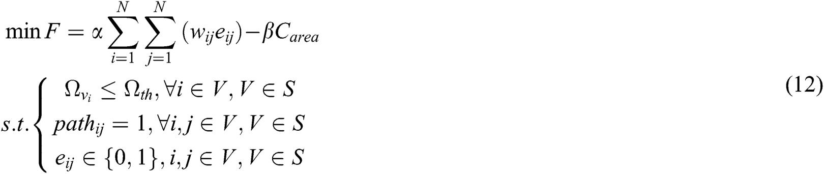
When the path loss between nodes vi and vj is less than threshold Prth, it is defined 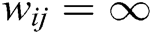 . The objective function that simultaneously optimizes network coverage and path loss is as Eq. (12). S represents the candidate sensor location set. V is the current location selected.
  ,
,  are the weight coefficient and
  represents the constraint on the number of forwarding.
  guaranteed that the communication probability between any two nodes vi, vj is 1. In addition, when the WSN logical topology contains the communication link between nodes vi and vj, eij = 1.
Then, this paper combines the tabu search algorithm and improved logical layout algorithm to solve Eq. (12). Tabu search algorithm is a heuristic algorithm simulating the human thinking process. It searches for the global solution by marking and avoiding local optimal solutions. First, the tabu search algorithm is used to select a given number of nodes from candidate locations to improve current network coverage. And the improved logical layout algorithm obtains network communication topology depending on the selected nodes under the forwarding constraint. Determine whether the local optimal objective function value is less than the global optimal solution, and update the physical layout and logical layout.
Traditional researches usually balance the network burden with the node-degree constraint. However, this paper studies a forwarding constraint. First, calculate the path loss between each node and other nodes depending on the maximum transmit power, and get the neighbor nodes of each node. Based on the adjacency matrix, the shortest path generation algorithm is used to obtain an initially logical network layout with the minimum path loss. Calculate the number of forwards for each forwarding node in the generated logical layout. If it is greater than the threshold, delete the direct link with the maximum path loss between this node and another node whose degree is not 1. The network logical layout is then regenerated until the forward constraint is met with minimal path loss.
The path loss experiment was conducted in No. 7 cucumber greenhouse, xiaotangshan national precision agriculture base, Beijing, China. The time was the cucumber fruit period with the most serious path loss. This greenhouse’s area is about  . In the greenhouse, each row was 0.5 m wide, with 15 plants, and the plant spacing was 0.3 m. The average cucumber height is about 1.7 m.
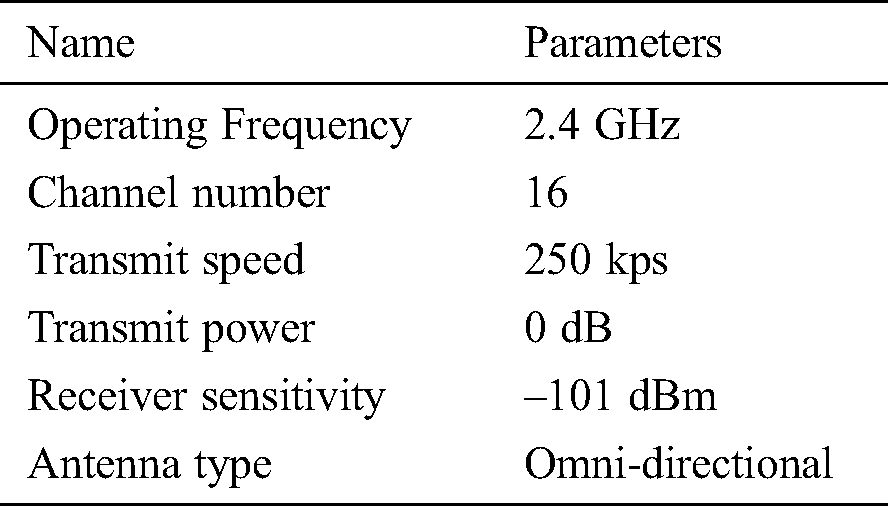
Both the transmitter nodes and receiver nodes use CC2530 wireless sensors which operate in 2.4 G frequency band. The node parameters are shown in Tab. 1.
(1) Node location: as shown in Fig. 2, place wireless nodes evenly in the greenhouse first packet trench, and use two packet trenches as a unit to make the transmitter nod es and receiver nodes at the same horizontal height.
(2) Node height: affected by plant growth, path loss in the greenhouses not only changes with location but also has certain differences at different heights. Therefore, we tested path loss at four heights according to the plant height with the same location, which are 0.5 m, 1 m, 1.5 m, and 2 m respectively. The channel quality at different heights is then obtained.
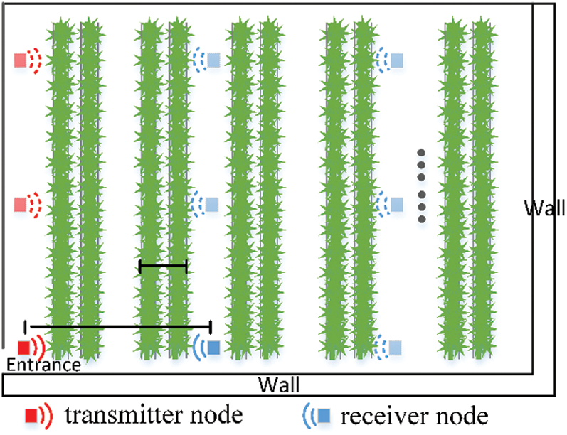
Figure 2: The schematic diagram of the experiment scheme
5.2.1 Path Loss in the Greenhouse
Fig. 3 shows the path loss data in different greenhouse locations. It can be seen that with the distance increase, RSSI (Received Signal Strength Indication) decreases gradually, but the decrease amplitude reduces with the distance increase. It will eventually decay to the receiver sensitivity. At different heights, the plant density is different, and the depth of the plant that the signal needs to cross is different. Therefore, RSSI varies with sensor heights. In Fig. 3, when the sensor height is 1 m and 0.5 m, the signal attenuation is severe due to the influence of plant occlusion and absorption. In this paper, the cucumber canopy is about 1.7 m, and it can be deduced that the fruits, stems and leaves are relatively mature at 1 m and 0.5 m. The signal loss increases with the increase of plant volume and density.
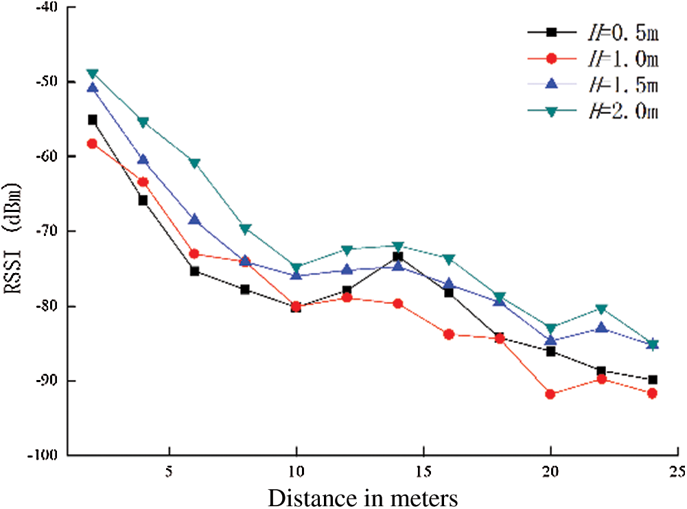
Figure 3: Measured data with different node heights
Taking 1.5 m height as an example, we use the existing vegetation model in Section 3.2 to predict path loss between different Tx-Rx distance. Figs. 4 and 5 shows predicted data and measured data. Compared with the combination of the FSPL model and vegetation models, the prediction errors for the combination of the two-ray model and vegetation models are larger, and the predicted data are generally smaller. Because the two-ray model only considers the main line-of-sight propagation and ground reflection rays of the signal, and there are walls, plastic ceiling, and other structures in the greenhouse, which leads to the signal multi-path propagation.
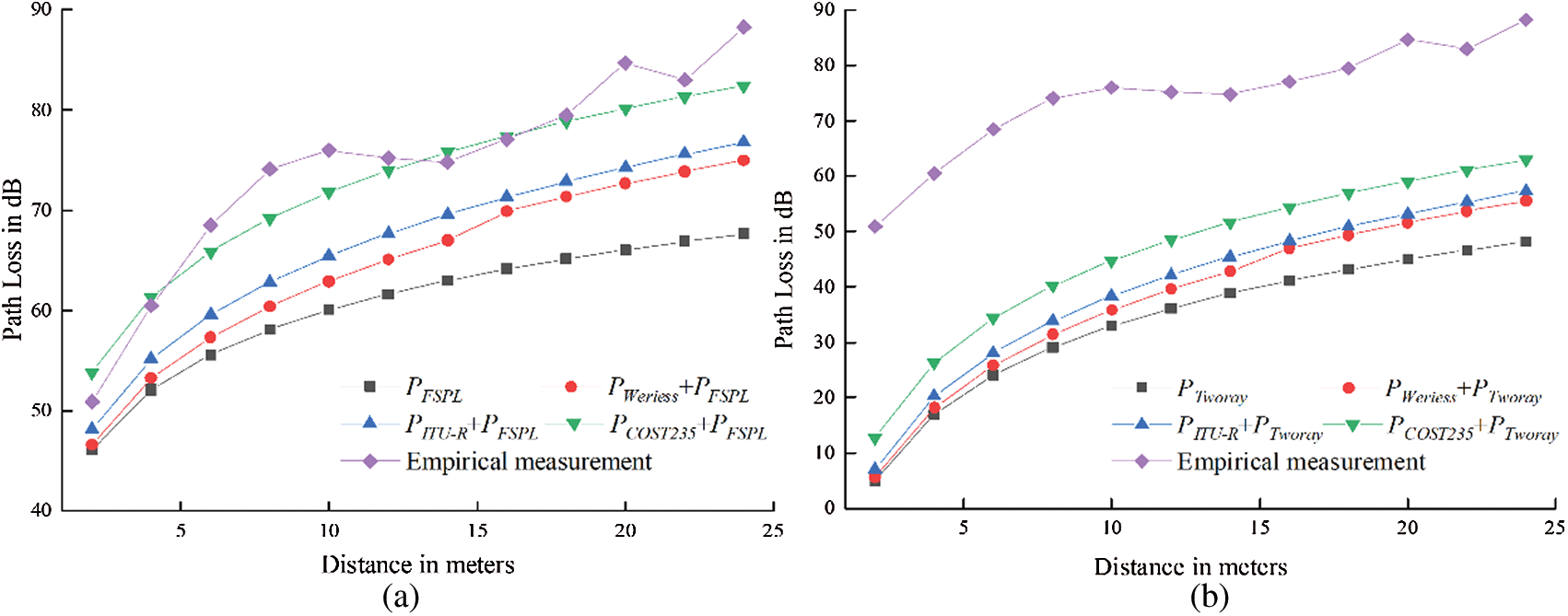
Figure 4: Measured empirical data at 1.5 m height vs empirical models combined with large-scale path loss models (a) Experimental data with antenna height at 1.5 m vs. FSPL model + empirical vegetation models (b) Experimental data with antenna height at 1.5 m vs. Two-ray model + empirical vegetation models
Tabs. 2 and 3 shows the relative error loss 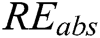 between the predicted data and measured data, which conforms to the trend in Figs. 4 and 5. The combination of the FSPL model and COST235 model can be close to the measured data, and the average relative error loss is only 3.2%, while the average error loss of the two-ray model combined with COST_235 model is 35.8%. We know that FSPL model can better predict the other factor (except vegetables) influence on the path loss.

where, y is the measured value, and yprecdict is the predicted value.
Table 2: The relative error between the data predicted by the FSPL model + empirical models and the measured data at 1.5 m height
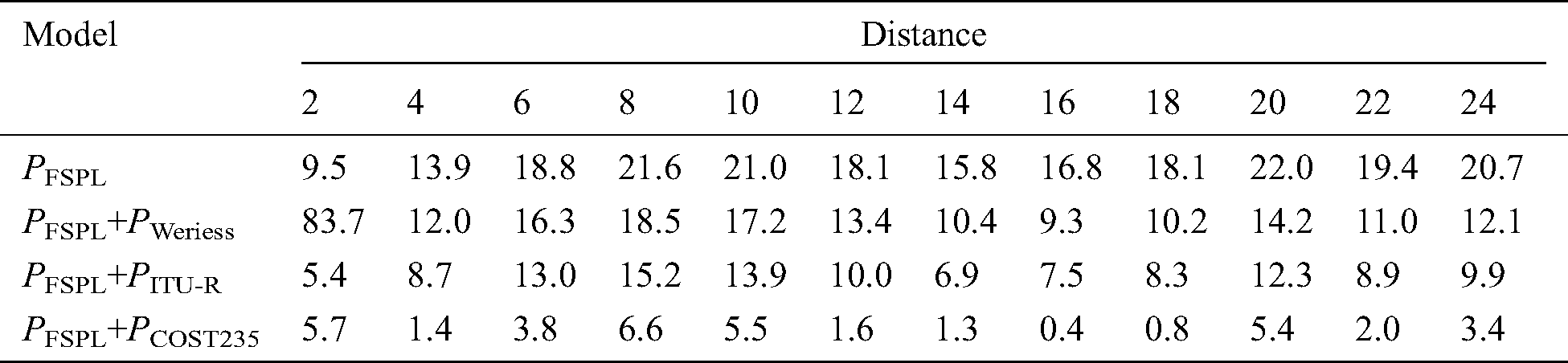
Table 3: The relative error between the predicted data of the two-ray model + empirical models and the measured data at 1.5 m height
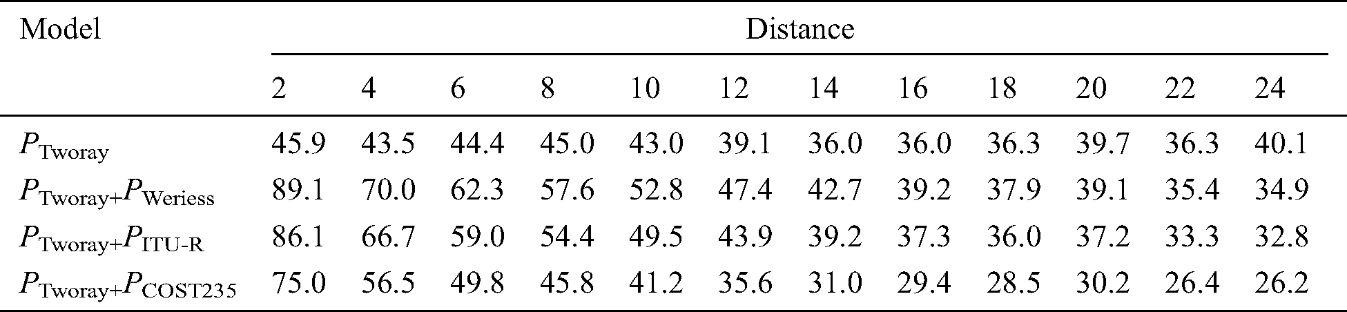
Although the combination of the FSPL model and COST 235 model performs a good prediction, it still has a significant error. From the above, the prediction effect of the FSPL model combined with other vegetation models is better than that of the two-ray model combined with other models. Therefore, based on the FSPL model, the least square method is used for fitting model parameters according to Eqs. (7) and (8). The results are as Tab. 4.
The new regression fitting model can achieve a smaller relative error loss of 2.3%. It accords with the characteristics of signal transmission and attenuation in the vegetable greenhouse.
Table 4: The fitting results of the model in this paper
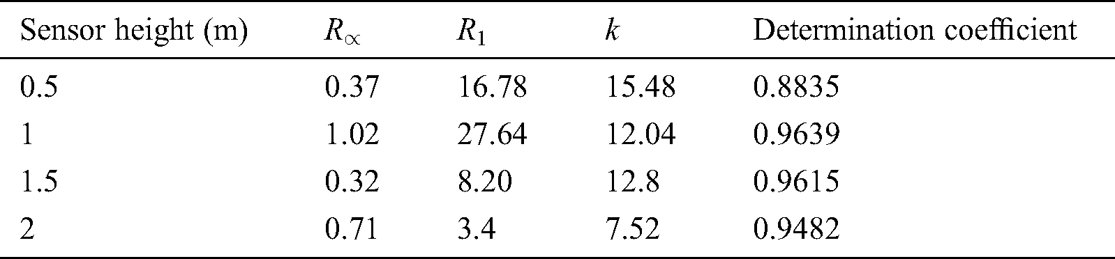
Semi-empirical model fitting is carried out for the measured signals at the heights of 0.5 m, 1 m, 1.5 m, and 2 m, respectively. The regression parameters are shown in Tab. 5. The determination coefficient determines the correlation between the fitting equation and the measured data. The closer it is to 1, the higher the reference value of the fitting expression. The determination coefficient shown in Tab. 5 indicates that for sensors at different heights, a stable greenhouse wireless signal path loss model can be fitted in this paper.
Table 5: Regression parameters of semi-empirical path loss model
5.2.2 Layout Simulation of Greenhouse WSN Based on Path Loss
We simulate 6 sensor nodes with a sensing radius of 3 m in the greenhouse for accurate sensing. By calculating, the maximum coverage that can be achieved is 0.92. In this section, the signal transmission at 1.5 m is taken as an example to analyze the performance of our optimization algorithm for WSN layout. According to Section 5.1, the path loss between sensors at 1.5 m height is:

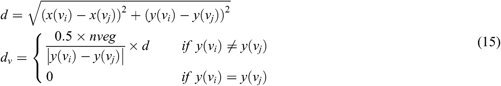
When the path loss is greater than 80 dB, the corresponding nodes are considered to be disconnected. In addition, d is the distance between vi, vj. dv is the vegetable depth that the signal crosses:
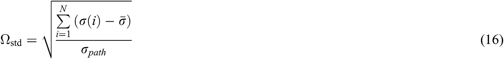
Taking the path loss between nodes as the edge weight in Eq. (12), we utilize the tabu search algorithm and improved topology method to get the WSN layout at 1.5 m. Fig. 10b shows the physical distribution of wireless sensor nodes in the greenhouse, and Fig. 9b shows the corresponding logical layout. In order to verify the studied algorithm performance, this paper first compares it with the network topology algorithm without the forwarding constraint and the maximal coverage hybrid search algorithm (MCHSA) in Panag et al. [19]. The comparison indexes include average node-degree, average path hops and so on. For each node’s energy consumption pressure, this paper uses the standard deviation between the shortest path number experienced by each node and the mean value of the shortest path to measure:
As shown in Tab. 6, three algorithms can obtain the greenhouse network layouts with good effective coverage, same average node-degree and same average hop number. The standard deviation of our algorithm is small, indicating that the energy consumption balance is improved, which provides a good foundation for subsequent network life extension. Fig. 5 shows the optimized network layout of three algorithms. In Fig. 5b, with node 3 as the forwarding node, the paths with minimum signal loss are:  ,
,  , four times in total. In order to reduce the forwarding times of node 3, this algorithm obtains the asymmetric shortest communication paths:
  ,
,  ,
,  ,
,  , which reduces the energy consumption of node 3. The Fig. 5c shows that after MCHSA determines the node locations, the network layout obtained by the improved algorithm also optimizes the node forwarding times. However, since the path loss is not considered in the physical layout, the path loss and average path energy consumption is worse.
Table 6: Performance comparison between our algorithm and other algorithms
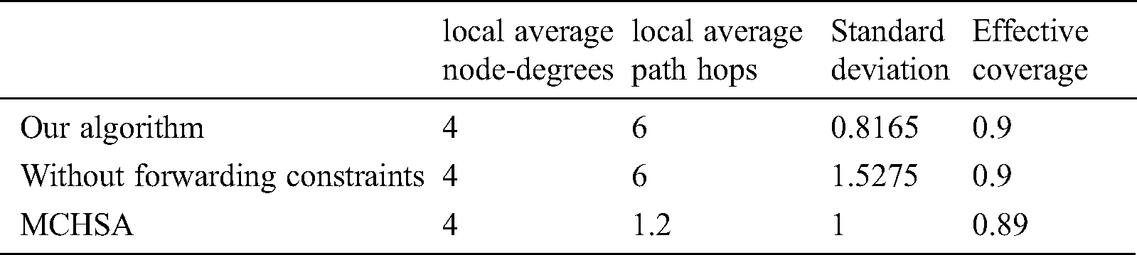
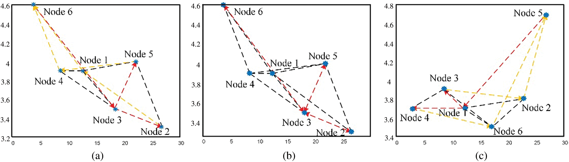
Figure 5: Network layouts formed by different algorithms (a) the topology obtained by our algorithm, (b) the topology obtained by the algorithm without forwarding constraint, (c) the topology obtained by the MCHSA algorithm with forwarding constraint
The WSN lifetime is related to many factors such as routing protocol and the MAC protocol. In order to further verify our algorithm effectiveness, we set a node as the sink node and the other nodes as the common nodes. Then we test the energy consumption of the three algorithms.
In Figs. 6a and 6b, the residual energy and standard deviation are compared. Our algorithm has the maximum residual energy and the minimum residual energy standard deviation. The algorithms without the forwarding constraint has a large standard deviation, although the residual energy trend is similar to that of our algorithm. MCHSA algorithm has smaller residual energy standard deviation, but less residual energy. With the increase of rounds, our algorithm has more obvious advantages than the other two algorithms. Fig. 7 shows the residual energy of each node at the 20th round. The algorithm in this paper makes the residual energy between nodes more balanced and improves the average residual energy by consuming more energy of some nodes. Fig. 8 shows the death round of the first node in three algorithms. Compared with the other two algorithms, our algorithm can effectively prolong the node death time and reduce the energy consumption depending on the forwarding constraint and physical location optimization.
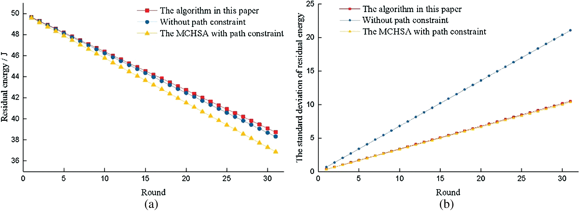
Figure 6: Network energy comparison of different algorithms
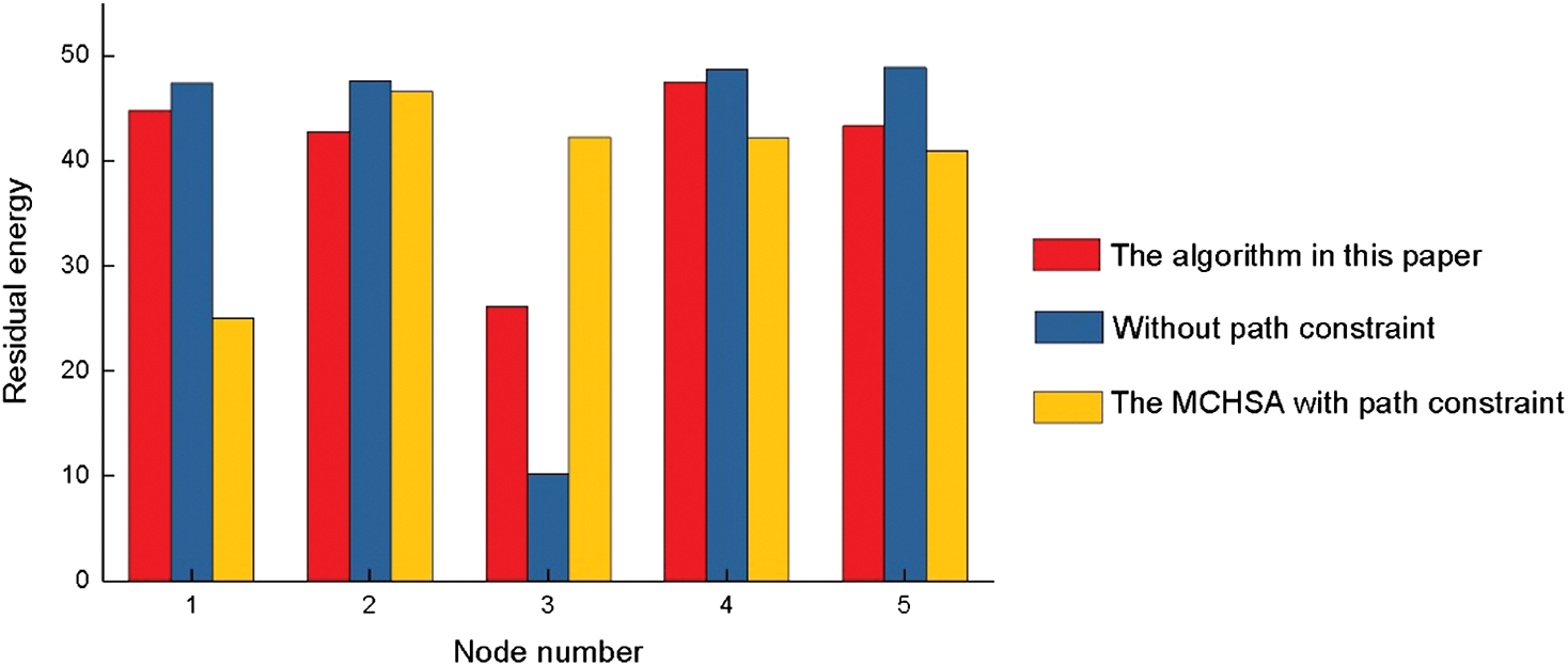
Figure 7: Residual energy of each node in the 20th round
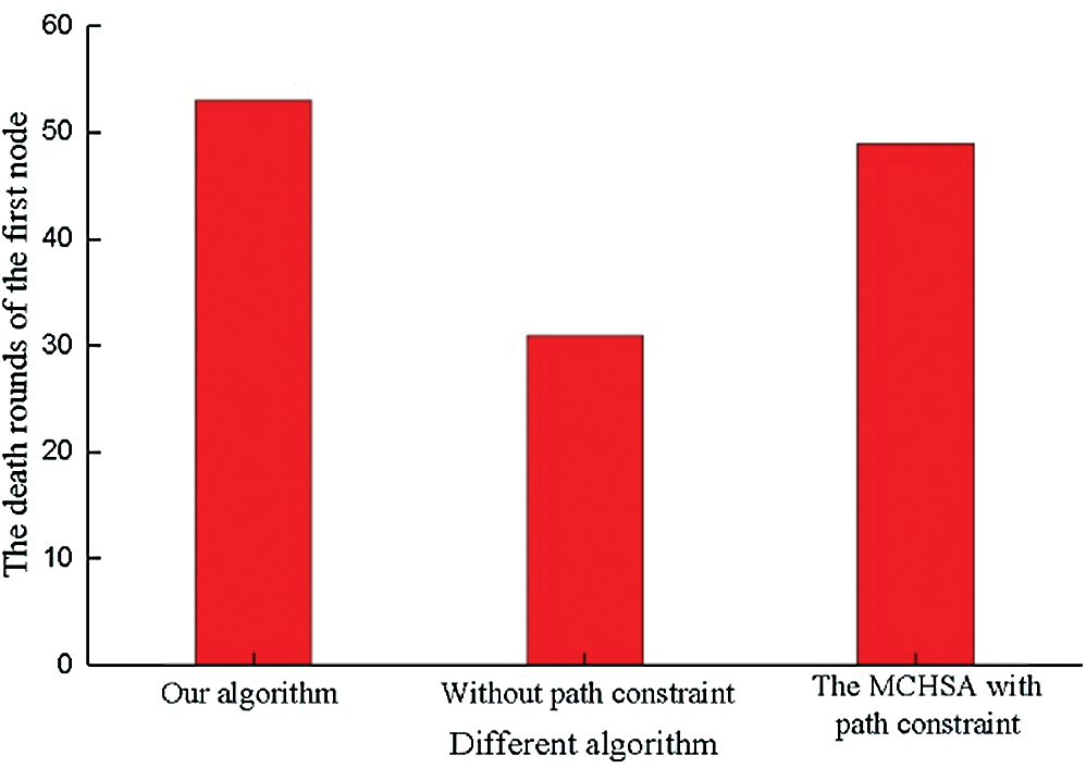
Figure 8: The death round of the first node
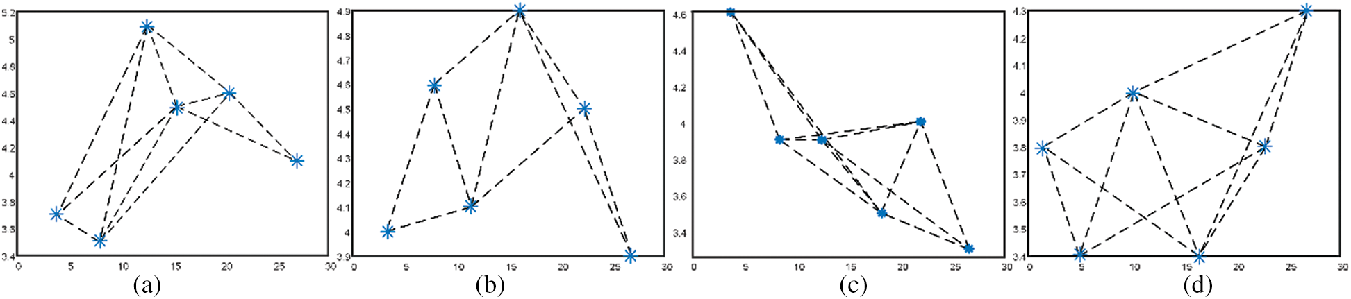
Figure 9: Network layout at different sensor heights (a) Wireless network topology in greenhouse with antenna height of 0.5 m (b) Wireless network topology in greenhouse with antenna height of 1.0 m (c) Wireless network topology in greenhouse with antenna height of 1.5 m (d) Wireless network topology in greenhouse with antenna height of 2.0 m
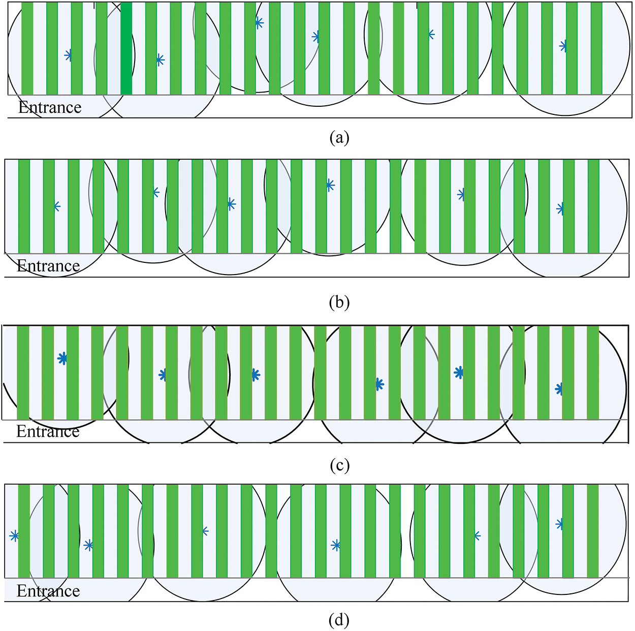
Figure 10: Network physical layout in the greenhouse at different sensor heights (a) Wireless network layout in greenhouse with antenna height of 0.5 m (b) Wireless network layout in greenhouse with antenna height of 1.0 m (c) Wireless network layout in greenhouse with antenna height of 1.5 m (d) Wireless network layout in greenhouse with antenna height of 2.0 m
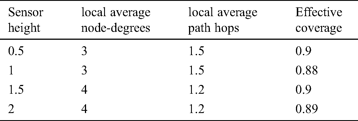
In addition, we verify our algorithm performance when the sensor height is 0.5 m, 1 m, 1.5 m, and 2.0 m respectively. The physical layout can cover an area as large as possible and forms a connected logical layout that can communicate between any two nodes. According to Section 5.1, when the height is lower, the signal path loss is greater due to the higher density of fruits and leaves. In Tab. 7, when the height is 0.5 m and 1 m, the average node-degree and local path average hops are relatively more. Our algorithm can get a layout scheme of WSN suitable for the greenhouses according to the actual application demand.
Table 7: Network logical layout performance at different sensor heights
In order to promote the practical application of WSN, this study discusses the extra signal loss caused by vegetables in the greenhouse. The path loss under different Tx-Rx distances is measured, and it is found that there is a relative error between the measured path loss and data predicted by vegetation models. A semi-empirical model established in this paper can more express the signal path loss in the greenhouse accurately. Based on this model, we improved the greenhouse WSN layout, which includes the physical and logical layout. Compared with the existing network layout algorithm, this paper replaces the node-degree constraint with the forwarding constraint and realizes the better greenhouse WSN construction by combining the tabu search algorithm and improved topology method.
Our further work mainly includes applying the research to practical application and measuring actual energy consumption about the optimized greenhouse WSN. In addition, considering the monitoring needs, different receivers and transmitters may have different height requirements, so we plan to develop research on the signal path loss characteristics and layout optimization in a three-dimensional environment.
Funding Statement: This work was funded by the National Natural Science Foundation of China (grant number 61871041); Technical System of the National Bulk Vegetable Industry (grant number CARS-23-C06).
Conflicts of Interest: The authors declare no conflict of interest.
1. D. P. Rubanga, K. Hatanaka and S. Shimada. (2019). “Development of a simplified smart agriculture system for small-scale greenhouse farming,” Sensors and Materials, vol. 31, no. 3, pp. 831–843. [Google Scholar]
2. S. Vougioukas, H. T. Anastassiu, C. Regen and M. Zude. (2013). “Influence of foliage on radio path losses (PLs) for wireless sensor network (WSN) planning in orchards,” Biosystems Engineering, vol. 114, no. 4, pp. 454–465. [Google Scholar]
3. Y. H. Ji, Y. Q. Jiang, T. Li, M. Zhang, S. Sha et al. (2016). , “An improved method for prediction of tomato photosynthetic rate based on WSN in greenhouse,” International Journal of Agricultural and Biological Engineering, vol. 9, no. 1, pp. 146–152. [Google Scholar]
4. C. C. Baseca, S. Sendra, J. Lloret and J. Tomas. (2019). “A smart decision system for digital farming,” Agronomy-Basel, vol. 9, no. 5, pp. 216. [Google Scholar]
5. Y. Mekonnen, S. Namuduri, L. Burton, A. Sarwat and S. Bhansali. (2020). “Review-machine learning techniques in wireless sensor network based precision agriculture,” Journal of The Electrochemical Society, vol. 167, no. 3, pp. 037522. [Google Scholar]
6. A. Catini, L. Papale, R. Capuano, V. Pasqualetti, D. Di Giuseppe et al. (2019). , “Development of a sensor node for remote monitoring of plants,” Sensors, vol. 19, no. 22, pp. 4865. [Google Scholar]
7. A. Khattab, S. E. D. Habib, H. Ismail, S. Zayan, Y. Fahmy et al. (2019). , “An IoT-based cognitive monitoring system for early plant disease forecast,” Computers and Electronics in Agriculture, vol. 166, pp. 105028. [Google Scholar]
8. I. Picallo, H. Klaina, P. Lopez-Iturri, E. Aguirre, M. Celaya-Echarri et al. (2019). , “A radio channel model for D2D communications blocked by single trees in forest environments,” Sensors, vol. 19, no. 21, pp. 4606. [Google Scholar]
9. S. M. Zhang, M. Madadkhani, M. Shafieezadeh and A. Mirzaei. (2019). “A novel approach to optimize power consumption in orchard WSN: Efficient opportunistic routing,” Wireless Personal Communications, vol. 108, no. 3, pp. 1611–1634. [Google Scholar]
10. D. Cama-Pinto, M. Damas, J. A. Holgado-Terriza, F. Gomez-Mula and A. Cama-Pinto. (2019). “Path loss determination using linear and cubic regression inside a classic tomato greenhouse,” International Journal of Environmental Research and Public Health, vol. 16, no. 10, pp. 1744. [Google Scholar]
11. A. Raheemah, N. Sabri, M. S. Salim, P. Ehkan and R. B. Ahmad. (2016). “New empirical path loss model for wireless sensor networks in mango greenhouses,” Computers and Electronics in Agriculture, vol. 127, pp. 553–560.
12. T. O. Olasupo and C. E. Otero. (2020). “The impacts of node orientation on radio propagation models for airborne-deployed sensor networks in large-scale tree vegetation terrains,” IEEE Transactions on Systems, Man, and Cybernetics: Systems, vol. 50, no. 1, pp. 256–269. [Google Scholar]
13. M. A. Weissberger. (1982). “An initial critical summary of models for predicting the attenuation of radio waves by trees.” Annapolis, MD, USA: Electromagnetic Compatibility Analysis Center, . [Online]. Available: https://www.zhangqiaokeyan.com/ntis-science-report_other_thesis/020711608124.html. [Google Scholar]
14. T. S. Rappaport. (1996). “Mobile radio propagation: Large-scale path loss,” in Wireless Communications: Principle and Practice, NJ United States, USA: Prentice Hall PTR, chapter 3, section 2, pp. 70–73. [Google Scholar]
15. J. Richter, R. F. S. Caldeirinha, M. O. Al-Nuaimi, A. Seville, N. C. Rogers et al. (2005). , “A generic narrowband model for radiowave propagation through vegetation,” in 2005 IEEE 61st Vehicular Technology Conference, Stockholm, Sweden. [Google Scholar]
16. W. Yi and C. Guohong. (2011). “On full-view coverage in camera sensor networks,” in 2011 Proc. IEEE INFOCOM, Shanghai, China, pp. 1781–1789. [Google Scholar]
17. A. Adulyasas, Z. L. Sun and N. Wang. (2015). “Connected coverage optimization for sensor scheduling in wireless sensor networks,” IEEE Sensors Journal, vol. 15, no. 7, pp. 3877–3892. [Google Scholar]
18. J. Wang, C. W. Ju, Y. Gao, A. K. Sangaiah and G. J. Kim. (2018). “A PSO based energy efficient coverage control algorithm for wireless sensor networks,” Computers Materials & Continua, vol. 56, no. 3, pp. 433–446. [Google Scholar]
19. T. S. Panag and J. S. Dhillon. (2019). “Maximal coverage hybrid search algorithm for deployment in wireless sensor networks,” Wireless Networks, vol. 25, no. 2, pp. 637–652. [Google Scholar]
20. X. C. Dang, C. G. Shao and Z. J. Hao. (2019). “Target detection coverage algorithm based on 3D-voronoi partition for three-dimensional wireless sensor networks,” Mobile Information Systems, vol. 2019, pp. 1–15. [Google Scholar]
21. T. T. Nguyen, J. S. Pan and T. K. Dao. (2019). “An improved flower pollination algorithm for optimizing layouts of nodes in wireless sensor network,” IEEE Access, vol. 7, pp. 75985–75998. [Google Scholar]
22. P. Adasme. (2019). “Optimal sub-tree scheduling for wireless sensor networks with partial coverage,” Computer Standards & Interfaces, vol. 61, pp. 20–35. [Google Scholar]
23. L. L. Wang, F. Xiao and C. Huang. (2019). “Adaptive topology control with link quality prediction for underwater sensor networks,” Ad Hoc & Sensor Wireless Networks, vol. 43, no. 3–4, pp. 179–212. [Google Scholar]
24. X. L. Li, B. Keegan, F. Mtenzi, T. Weise and M. Tan. (2019). “Energy-efficient load balancing ant based routing algorithm for wireless sensor networks,” IEEE Access, vol. 7, pp. 113182–113196. [Google Scholar]
25. A. Kannagi. (2018). “K-Partitioned smallest distance mining tree for path optimation in wireless sensor network,” Wireless Personal Communications, vol. 103, no. 4, pp. 3099–3112. [Google Scholar]
26. S. S. Banihashemian, F. Adibnia and M. A. Sarram. (2018). “Proposing a measurement criterion to evaluate the border problem in localization algorithms in WSNs,” Computing, vol. 100, no. 12, pp. 1251–1272. [Google Scholar]
27. M. Mirhosseini, F. Barani and H. Nezamabadi-pour. (2017). “Design optimization of wireless sensor networks in precision agriculture using improved BQIGSA,” Sustainable Computing: Informatics & Systems, vol. 16, pp. 38–47. [Google Scholar]
28. M. R. Senouci and A. Mellouk. (2019). “A robust uncertainty-aware cluster-based deployment approach for WSNs: Coverage, connectivity, and lifespan,” Journal of Network and Computer Applications, vol. 146, pp. 102414. [Google Scholar]
29. A. Seville. (1997). “Vegetation attenuation: modelling and measurements at millimetric frequencies,” in Tenth Int. Conf. on Antennas and Propagation, Edinburgh, UK, pp. 5–8. [Google Scholar]
 | This work is licensed under a Creative Commons Attribution 4.0 International License, which permits unrestricted use, distribution, and reproduction in any medium, provided the original work is properly cited. |
