New Soliton Wave Solutions to a Nonlinear Equation Arising in Plasma Physics

1  Introduction

Many natural and physical processes can be effectively described using partial differential equations (PDEs). For example, plasma physics, vibrations in materials, population growth, the flow of liquids and gases, electromagnetic fields, waves in liquids, radiation, optical fibers, heat transfer, and others can be efficiently and successfully studied using PDEs. In particular, many significant oceanic phenomena have been explained by soliton propagation, including nonlinear shallow or deep sea wave propagation, transverse waves in shallow water, magneto hydrodynamic waves in plasma, and phonon packets in nonlinear crystals. PDEs provide a comprehensive explanation for the future behavior of such phenomena. The future behavior of these problems is well-known from the exact and numerical solutions of the corresponding PDEs. In other words, to better understand the long-term behavior of non-linear phenomena, it is consequential to explore their exact solutions. Therefore, the development of fundamental and systematic methods for deriving analytical solutions to PDEs has become a popular and fascinating subject for most scholars. Among these techniques, we propose the improved exp⁡(−Δ(ζ))-expansion method [1], the improved Kudryashov technique [2], the first integral technique [3], the generalized direct algebraic method [4], the improved Q-expansion method [5], the Jacobian elliptic functions technique [6], and more others. More information on various techniques and analytical solutions, including dark and light solitons, can be found in the references [7–18].

The generalized long wave (GRLW) equation [19] reads

Φt+Φx+c1ΦqΦx−c2Φxxt=0,(1)

where c1,c2 and q are positive integers and u represents the wave amplitude.

Eq. (1) is used to model the transverse waves in shallow water and the development of an undular bore. In addition, Eq. (1) plays an important role in physics as it is mainly used to study some phenomena involving dispersion waves such as magneto-hydrodynamic waves in plasma and ion-acoustic waves. The modified regularized long-wave equation (MRLW) [19,20], which is a special case of Eq. (1), reads as follows:

Φt+Φx+13(Φ3)x−Φxxt=0.(2)

Eq. (2) efficiently describes the propagation of nonlinear dispersive waves which occur in elastic rods and shallow water. This equation was analyzed in detail in various studies in terms of its numerical and exact solutions. For example, Bulut et al. [21] applied the effective Sine-Gordon expansion technique to search for soliton, optical wave and kink structures for Eq. (2). Pervin et al. [22] used the cosine function method to extract four traveling wave solutions for the MRLW equation. In [23], some numerical solutions for the MRLW equation were successfully obtained utilizing finite difference and finite element methods. The finite element approach was used by Karakoc et al. [24] to develop a collocation solution for Eq. (2). Also, the quartic B-spline collocation method was invoked in [25] to establish some numerical solutions for Eq. (2). Eq. (2) was also solved numerically in [26] via the collocation approach. In [24], a Petrov-Galerkin method with a cubic B-spline function was perfectly performed on Eq. (2) to investigate its numerical solutions. Jena et al. [27] took advantage of a quartic B-spline strategy with a fifth order Runge-Kutta scheme to develop a numerical solution for Eq. (2). Raslan et al. [28] derived some effective numerical results for the MRLW problem by using the finite element method. Khan et al. [29] approximated the numerical solutions of Eq. (2) by utilizing a homotopy analysis technique. Karakoç et al. [30] implemented a septic B-spline collocation method on Eq. (2) to obtain its numerical solution. The stability of the method was also discussed in [30]. Finally, Essa et al. [31] applied the multigrid approach and the finite difference method to Eq. (2) to extract one, two and three soliton solutions for the proposed equation. It can be noted that previous studies on Eq. (2) have mostly focused on finding the numerical solutions rather than seeking to reduce the resulting error. However, our study was able to reduce the error and acquire the numerical solutions of Eq. (2).

The motivation for this paper stems from the recent developments presented in the literature review. The main purpose of this paper is to develop some traveling wave solutions of the MRLW equation using the generalized algebraic technique, the Jacobian elliptic functions method, and the improved Q-expansion technique. The proposed methods have wonderful advantages, which are as follows. These methods provide a variety of reliable traveling wave solutions in the form of trigonometric, hyperbolic and rational expressions which can be utilized to interpret some complex phenomena. Moreover, the improved Q-expansion method can be easily utilized to treat nonlinear equations with variable coefficients [32]. This paper also aims to implement the adaptive moving mesh method on Eq. (2) to extract its numerical solutions. It is significant to mention that the initial condition of the numerical scheme is obtained from the constructed exact results. The main idea behind the used numerical method is to distribute the points in the curvature regions of the solutions. Despite the fact that numerous researchers work analytically to find the traveling wave solutions of the MRLW equation, only few scientists investigate the numerical solutions of this problem with a very small error. The points are fairly distributed in the areas with high error using the adaptive moving mesh approach. This procedure, which is not available on the majority of numerical algorithms, perfectly decreases the error. Hence, the numerical approach used is employed to generate accurate and dependable results. One of the greatest ways to ensure that the solutions are accurate is to check the conformity of exact and numerical solutions. Even though some experts only find exact solutions, in this study, we compare the exact and numerical solutions to ensure that the solutions are perfectly accurate and correct.

This article is structured as follows. Section 2 is devoted to the description of the proposed methods, namely, the generalized algebraic method, the Jacobian elliptic functions method, and the improved Q-expansion approach. In Section 4, we analyze the numerical solutions of the proposed problem. In Section 5, the main results are presented and discussed. Finally, Section 6 concludes this study.

2  Summary of Proposed Methods

We consider a nonlinear evolution equation with some physical fields Φ(x,t) in two variables x, and t as follows:

Ψ1(Φ,Φt,Φx,Φxxt,…)=0.(3)

Step 1. We seek explicit traveling wave solutions on the form

Φ=ϕ(ξ),  ξ=k(x−ct),(4)

where k and c are the wave number and wave speed, respectively.

Step 2. Using Eqs. (3) and (4) is directly reduced to

Ψ2(ϕ,ϕξϕξ,ϕξξξ,…)=0,

where Ψ2 is a polynomial in ϕ(ξ) and its derivatives.

2.1 Generalized Algebraic Method

According to the generalized direct algebraic method [4], the solution of Eq. (2) is given by

ϕ(ξ)=∑j=0Najψj+∑j=1N(bjψj+cj(ψψ′)j)+∑j=2Ndjψj−2ψ′,(5)

where aj, bj, cj, dj are to be determined, N is an integer number obtained by taking the balance between the highest degree of the nonlinear terms and the highest order of the derivatives and ψ(ξ) is a solution of the following differential equation:

ψ′(ξ)=ε∑j=0mqjψj(ξ),(6)

where ε is a parameter, m and qj are given in Table 1 in [4].

2.2 Improved Q-Expansion Method

The improved Q-expansion method [5] introduces the traveling wave solution of Eq. (2) on the form

ϕ(ξ)=A0+∑j=1N(Aj(μ+Q(ξ))j+Bj(μ+Q(ξ))j),(7)

where Aj, Bj and μ are to be evaluated later. The function Q(ξ) represents a solution of the following differential equation:

Q′(ξ)=γ0+γ1Q(ξ)+γ2Q(ξ)2,(8)

where γ0, γ1, γ2 are given in Table 1 in [5].

2.3 Jacobian Elliptic Functions Method

The Jacobian elliptic functions technique [6] gives the general form of the solution ϕ(ξ) by the following expression:

ϕ(ξ)=∑l=0Nalsnlξ,(9)

where

ϕ′(ξ)=∑l=0Nl alsnl−1ξ cnξ dnξ.(10)

Note that snξ, cnξ, dnξ are the Jacobian elliptic sine functions [6]. These functions have the following relations:

nsξ=1snξ, ncξ=1cnξ, ndξ=1dnξ, scξ=cnξsnξ,csξ=snξcnξ, dsξ=dnξsnξ, sdξ=snξdnξ.

Furthermore, these functions satisfy the following equations:

sn2ξ+cn2ξ=1, dn2ξ+m2sn2ξ=1, ns2ξ=1+cs2ξ,ns2ξ=m2+ds2ξ, sc2ξ+1=nc2ξ, m2sd2+1=nd2ξ,

where 0<m<1 is a modulus. In addition, the derivatives of the Jacobi elliptic functions are given by

sn′ξ=cnξdnξ, cn′ξ=−snξdnξ, dn′ξ=−m2snξcnξ.

ns′ξ=−dsξcsξ, ds′ξ=−csξnsξ, cs′ξ=−nsξdsξ.

sc′ξ=ncξdcξ, nc′ξ=scξdcξ, cd′ξ=cdξndξ, nd′ξ=m2sdξcdξ.

We can obtain a periodic solution with Jacobi elliptic functions when m→1. If m→1 we have that snξ tends to tanhξ. Hence, the periodic traveling wave solution is given by

ϕ(ξ)=∑j=0Najtanhj⁡ξ.(11)

3  Exact Solutions

In this section, the exact traveling wave solutions of Eq. (2) are found using three different methods. Applying Eq. (4) on Eq. (2) yields

3wk2ϕ″+ϕ3+3(1−w)ϕ=0.(12)

Balancing the highest order derivative ϕ″ and non-linear term ϕ3 leads to N=1.

3.1 Application of Generalized Direct Algebraic Method

In this subsection the traveling wave solutions of Eq. (2) are acquired using the generalized direct algebraic method. Since N=1, Eq. (5) becomes

ϕ(ξ)=a0+a1ψ(ξ)+b1ψ+c1ψψ′.(13)

Inserting Eq. (13) into Eq. (12) along with Eq. (6), we obtain a polynomial in ψ(ξ). Collecting the coefficient of ψ(ξ)j, (j=−3,−2,−1,0,1,2,3…), yields a system of algebraic equations. Solving this system obtains the values of a0, a1, b1, c1 and c as follows:

Case 1: When q2>0, q4<0, and q0=q1=q3=0 (see Table 1 in [4]), the values of the constants are given by

a0=0,a1=±εk6q4ε2kq2−1,b1=0,c1=0,c=11−ε2kq2,

and then the traveling wave solution is given by

Φ1(x,t)=±εk6q4ε2kq2−1(ε−q2q4sech(kq2(x−t1−ε2kq2))).

Case 2: When q2<0, q4>0, q0=q224q4, and q1=q3=0, the traveling wave solution is expressed as

Φ2(x,t)=±εk6q4ε2kq2−1(ε−q22q4tanh⁡(k−q22(x−t1−ε2kq2))).

Case 3: When q2>0, q4>0, q0=q224q4, and q1=q3=0, the traveling wave solution is shown by

Φ3(x,t)=±εk6q4ε2kq2−1(εq22q4tan⁡(kq22(x−t1−ε2kq2))).

Here, we take let k=1 and ε=±1 to ensure that the obtained solutions are correct.

3.2 Application of the Improved Q-Expansion Method

In this subsection, the traveling wave solutions of Eq. (2) are introduced using the improved Q-expansion method. Since N=1, Eq. (7) becomes

ϕ(ξ)=A0+A1(μ+Q(ξ))+B1(μ+Q(ξ)).(14)

Substituting Eq. (14) into Eq. (12) along with Eq. (8) yields a polynomial in Q(ξ) from which we collect the coefficient of Q(ξ)j, (j=0,1,2,…) to end up with a system of algebraic equations. Finding the solutions of this system gives the values of A0, A1, B1, and c as follows:

A0=±(23γ2μ4γ0γ2−γ12−2−3γ14γ0γ2−γ12−2),A1=∓23γ24γ0γ2−γ12−2,B2=0,c=2−4γ0γ2+γ12+2.

In order to make sure that the exact solution of Eq. (2) is correct, we let k=1.

Case 1: When γ0>0, γ1=0, γ2=1, the exact solutions are

Φ4(x,t)=±6μ2γ0−1∓62γ0−1(μ+γ0tan⁡(γ0(x−t1−2γ0))),Φ5(x,t)=±6μ2γ0−1∓62γ0−1(μ−γ0cot⁡(γ0(x−t1−2γ0))).

Case 2: When γ0<0, γ1=0, γ2=1, the exact solutions are

Φ6(x,t)=±6μ2γ0−1∓62γ0−1(μ−−γ0tanh⁡(−γ0(x−t1−2γ0))),Φ7(x,t)=±6μ2γ0−1∓62γ0−1(μ−−γ0coth⁡(−γ0(x−t1−2γ0))).

Case 3: When γ0=0, γ1=0, γ2=1, the exact solutions are

Φ8(x,t)=±6μ2γ0−1∓62γ0−1(μ−(1−2γ0)(1−2γ0)x−t).

3.3 Application of Jacobian Elliptic Function Expansion Approach

The essential aim of this part is to construct the traveling wave solutions of Eq. (2) using the Jacobian elliptic function expansion approach. Since N=1, Eq. (9) becomes

ϕ=a0+a1sn(ξ)+b1cn(ξ),(15)

where a0, a1 and b1 are constants. From Eq. (15), we can develop the derivatives of ϕ as follows:

ϕ′=a1cn(ξ)dn(ξ)−b1sn(ξ)dn(ξ),(16)

ϕ″=−m2sn(ξ)a1+2a1sn(ξ)3m2+2m2sn(ξ)2cn(ξ)b1−a1sn(ξ)−b1cn(ξ).(17)

Substituting Eqs. (15)−(17) into (12) and equating all coefficients of sn3, sn2cn, sn2, sncn, sn, cn, sn0 to zero lead to the following system:

6wk2m2a1+(a13−3a1b12)=0,

6wk2m2b1+(3a12b1−b13)=0,

a0(a12−b12)=0,

a0a1b1=0,

3wk2a1(−1−m2)+(3a02a1+3a1b12)+3(1−w)a1=0,

−3wk2b1+(3a02b1+b13)+3(1−w)b1=0,

(a03+3a0b12)+3(1−w)a0=0.

Solving the above system, we obtain the values of a0,a1,b1 and w as given in the following cases:

Case 1:

a0=0,a1=0,b1=±6wkm,w=11+k2(1−2m2).

As long as m→1, the traveling wave solutions of Eq. (2) is degenerated by

Φ9(x,t)=±6wksech(k(x−wt)),w=11−k2.(18)

Case 2:

a0=0,a1=±3km−2+k2(m2−2),b1=−3km2+k2(2−m2),w=−2−2+k2(m2−2).

As long as m→1, the traveling wave solutions of Eq. (2) is degenerated by

Φ10(x,t)=±3k−2−k2tanh(k(x−wt))−3k2+k2sech(k(x−wt)),w=22+k2.

Case 3:

a0=0,a1=±3km−2+k2(m2−2),b1=3km2+k2(2−m2),w=−2−2+k2(m2−2).

As long as m→1, the traveling wave solutions of Eq. (2) is shown as

Φ11(x,t)=±3k−2−k2tanh(k(x−wt))+3k2+k2sech(k(x−2t2+k2)).

Case 4:

a0=0,a1=±6km−1−k2(1+m2),b1=0,w=11+k2(1+m2).

As long as m→1, the traveling wave solutions of Eq. (2) is written as

Φ12(x,t)=6k−1−2k2tanh(k(x−t1+2k2)).(19)

4  Numerical Results

Eq. (2) is discretised by applying a non-uniform mesh scheme, which will be discussed later. The derivation of this problem is obtained from some boundary conditions and the initial data which is taken by the exact solution Eq. (18) at t=0. Next, the finite difference technique and the method of lines are employed to find the numerical solution to this problem and discover the evolution of Φ(x,t). In our investigation explained below, we take the values of the parameters as follows: k=0.5, w=1/(1−k2), a=−20, and b=30. Then, the numerical solutions obtained by the uniform mesh and an adaptive moving mesh will be compared in terms of their convergence and accuracy.

4.1 Numerical Results on an Adaptive Mesh

In this subsection, we analyze the numerical solution of Eq. (2) using the adaptive moving mesh approach. The basic idea of the r-adaptive moving mesh techniques is to perfectly distribute the points on the variations of the solution [33]. Based on the equidistribution principle, many MMPDEs have been developed for time-dependent problems [34,35]. Huang et al. [36] and Budd et al. [34] have presented several continuous formulas for MMPDEs formed using the coordinate transformation and a monitor function. An appropriate choice of the monitor function often leads to good performance for the adaptive moving mesh approaches. We use the following boundary conditions:

Φx(a,t)=Φx(b,t)=0,Φxx(a,t)=Φxx(b,t)=0,(20)

where a and b are the end points of the physical domain. Moreover, the initial condition is established by evaluating the Eq. (18) at t=0. Eq. (18) is used when t=5 to investigate the accuracy and convergence of the computed solution using an adaptive moving mesh and the uniform mesh. Consider the coordinate transformation x=x(ξ,t):[0,1]→[a,b], t>0, where x denotes the physical coordinate, and ξ is the computational coordinate. Then, the solution is expressed as Φ(x,t)=Φ(x(ξ,t),t). Therefore, a moving mesh related to the solution Φ is formed as 𝒥h(ts):xj(ξ)=x(ξj,t), j=1,⋯,N+1, where the boundary mesh is provided by x1=ξ1,  xN+1=(b−a)ξN+1. A uniform mesh on the computational domain is given by 𝒥hc(t):ξj=(j−1)/N, j=1,⋯,N+1. We now use the chain rule on Eq. (2) to have

qt=Φξxξxt−fξxξ,(21)

q=Φ−1xξ(Φξxξ)ξ,(22)

f=Φ+Φ33.(23)

We then represent the boundary conditions in terms of the ODEs as follows: Φt,1=0,Φt,N+1=0, and the initial condition is assumed by Eq. (18) at t=0. Note that x(ξ) can be generated using MMPDEs [33,35,37]. The MMPDE6 is used in this work to obtain more reliable solutions. The semi-discretisation of MMPDE6 was developed in [33,37] as

MMPDE6:(xt,i+1−2xt,i+xt,i−1)=−1τ(ρ^i+1/2(xi+1−xi)−ρ^i−1/2(xi−xi−1)),

where ρ^(x,t) represents a monitor function, ρ^i+1/2=(ρ^i+1+ρ^i)/2, ρ^i−1/2=(ρ^i+ρ^i−1)/2 and τ∈(0,1) is a relaxation constant. The boundary conditions are shown as xt,1=0,xt,N+1=0 and the initial uniform mesh is taken by x(ξ,0)=(b−a)(j−1)/N,j=1,2,…,N+1. Finally, the monitor function ρ^(x,t) is selected as follows:

Curvature monitor function:ρ^(x,t)=1+α|ux|2,(24)

where α is a positive constant. Using a smooth function ρ^ is necessarily needed to enrich regular meshes [33,35,37]. Therefore, we execute the resulting low-pass filter double

ρ^i,j←ρ^i,j+1/8(ρ^i+1,j+ρ^i−1,j+ρ^i,j+1+ρ^i,j−1)+1/16(ρ^i+1,j+1+ρ^i−1,j−1+ρ^i−1,j+1+ρ^i+1,j−1).(25)

Fig. 1 shows time evolution of Φ(x,t) and its associated mesh x(ξ,t) obtained by applying the adaptive moving mesh scheme with N=1000.

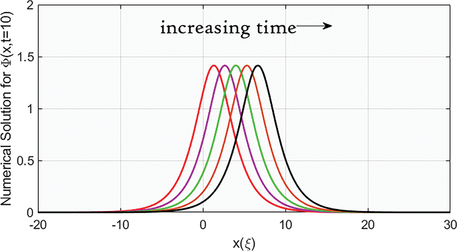
Figure 1: This figure presents time evolution (time t=0−10) of the solution Φ(x,t). The parameter values α=10, k=0.5, N=1000 and time t increasing among 0 and 10.

5  Results and Discussion

This section is to highlight the main results of this work. We use the generalized algebraic approach, the technique of elliptic Jacobian functions, and the improved Q-expansion approach to produce the exact solutions of Eq. (2). We also implement the adaptive moving mesh approach to extract the numerical solutions to the proposed problem.

Comparisons are perfectly made between the analytical solutions obtained and those from other studies. In [22], the authors developed four traveling wave solutions for the MRLW equation using the cosine function method. These solutions were given in terms of an inverse cosine function. In contrast, we use methods that provide multiple solutions in different forms. For example, the generalized direct algebraic approach provides many traveling wave solutions in the form of trigonometric functions and hyperbolic functions. Additionally, the improved Q-expansion process leads to abounding solutions in the form of trigonometric and hyperbolic functions. We can conclude that the used methods provide more traveling wave solutions than the cosine function method.

The obtained numerical solution of Eq. (2) coincides with the exact solution of this equation, as can be seen in Fig. 2a. Fig. 2a illustrates a single soliton solution to Eq. (2). Fig. 2b displays the curvature monitor function associated with the numerical solution presented in Fig. 2a. In Fig. 2b, we plot two solitary waves with the same amplitude when t=10. Moreover, in Figs. 3a and 3b, we observe that the numerical solution of Eq. (18) nearly behaves like its exact solution under the used parameter values which are k=0.5, w=4/3, a=−20, b=30, N=500, τ=10−4 and α=10. Fig. 4c presents the curvature-based mesh density function associated with the solutions. Fig. 4d presents the time evolution of the equidistributing coordinate transformation x(ξ,t).

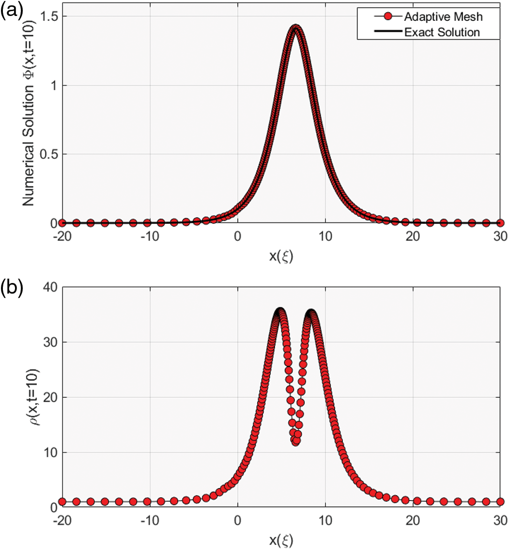
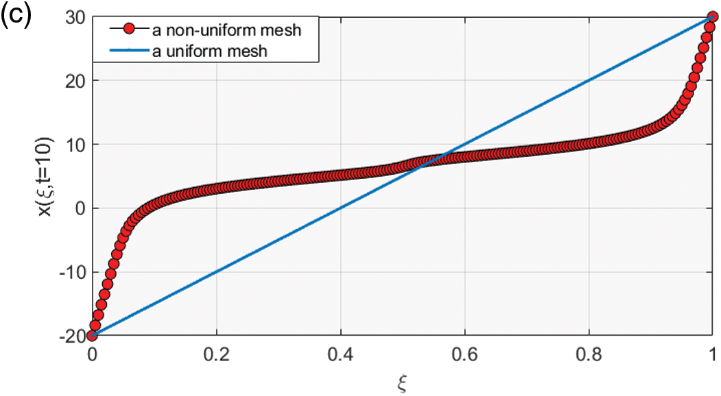
Figure 2: (a) shows a single wave for the exact and numerical solutions of Φ(x,t=10). (b) Illustrates curvature-based density function and (c) depicts development of time using a non-uniform mesh and a uniform mesh. The parameter values are given by α=10, k=0.5, N=1000.

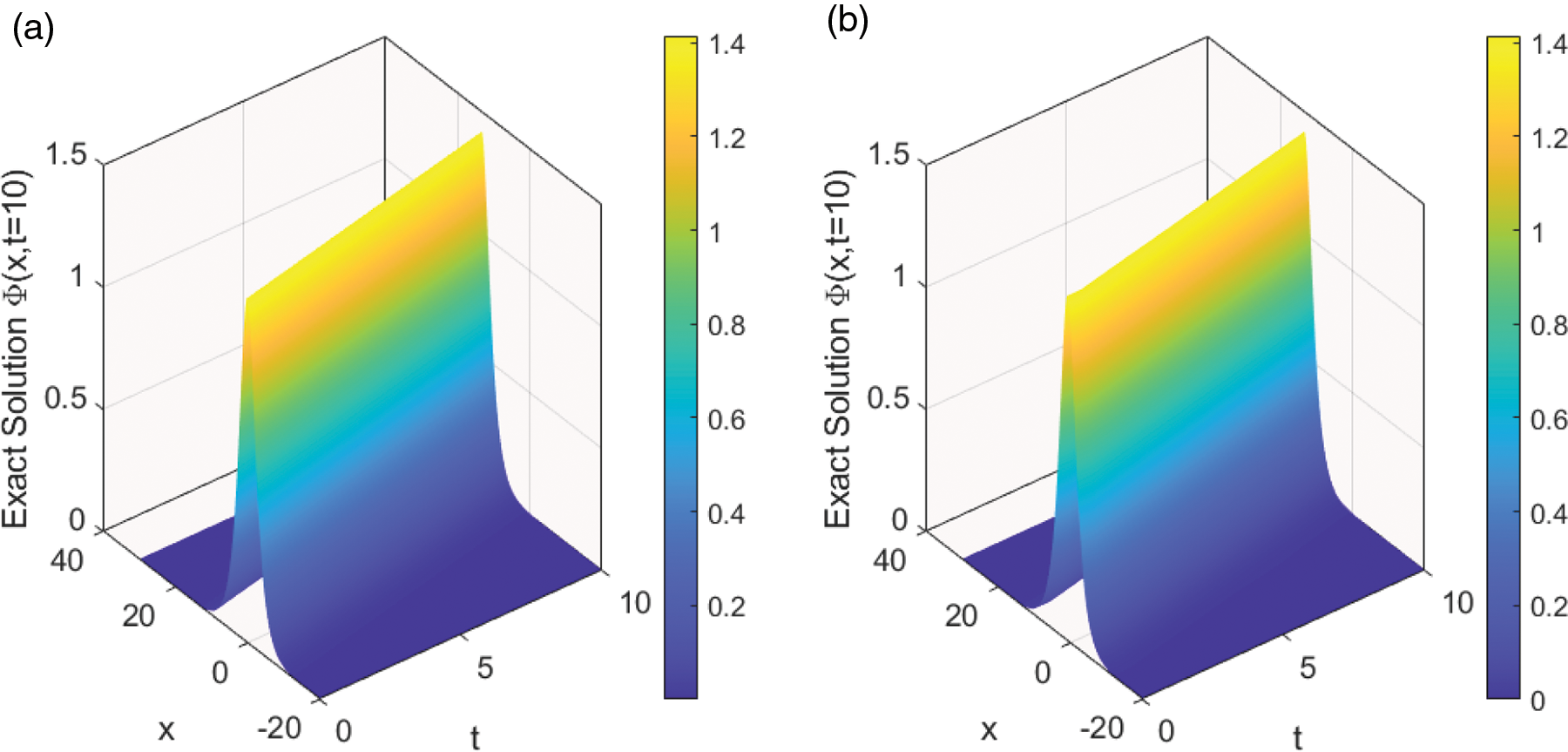
Figure 3: A pulse exact solution of Eq. (18) is shown in the left figure while the right figure presents the numerical solution of this equation. The parameter values are taken by k=0.5, w=4/3, a=−20, b=30, N=1000, τ=10−4, α=10 and time t increasing between 0 and 10.

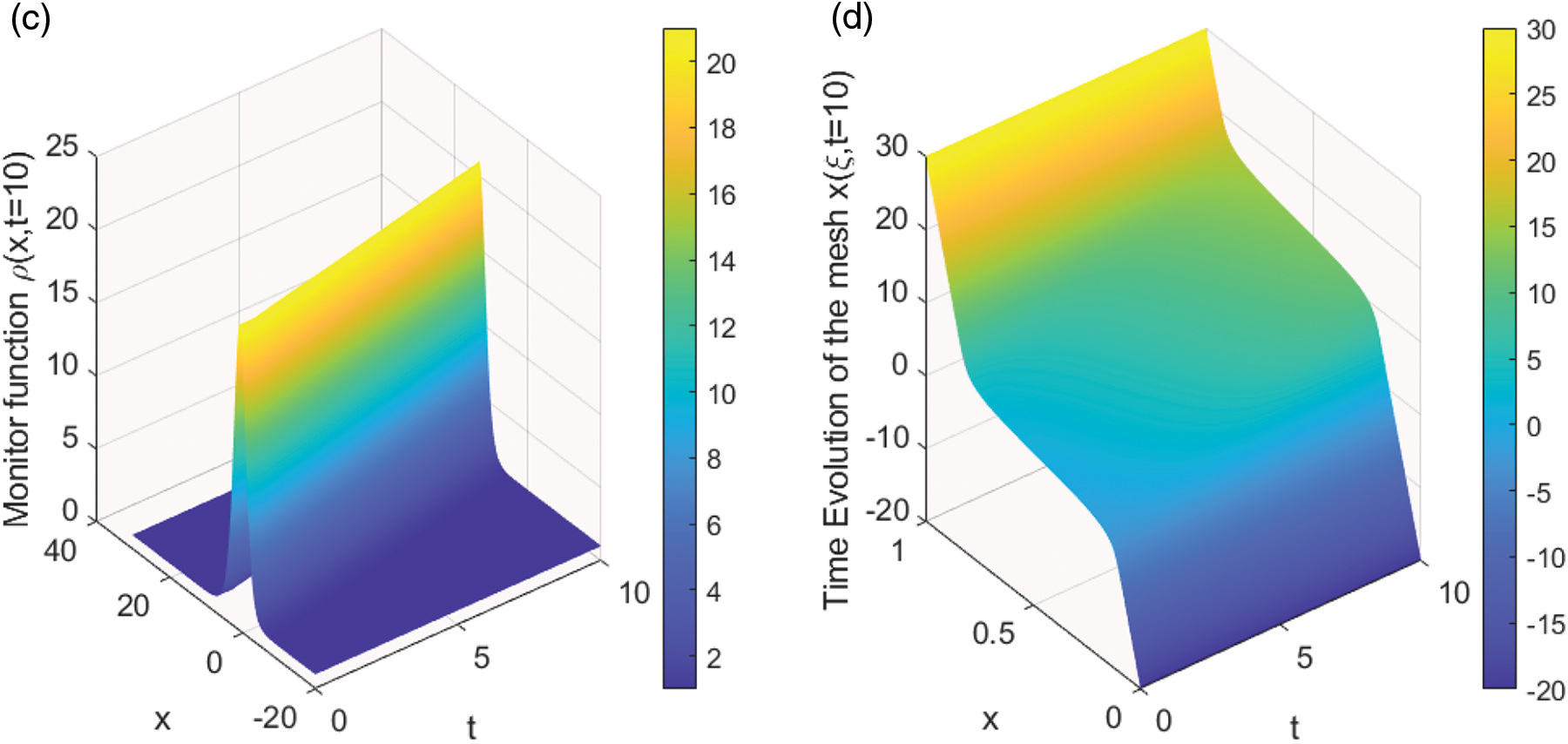
Figure 4: The left plot illustrates the time evolution of the monitor function while the right graph depicts the time evolution of the mesh. The parameter values are taken by k=0.5, w=4/3, a=−20, b=30, N=1000, τ=10−4, α=10 and time t increasing between 0 and 10.

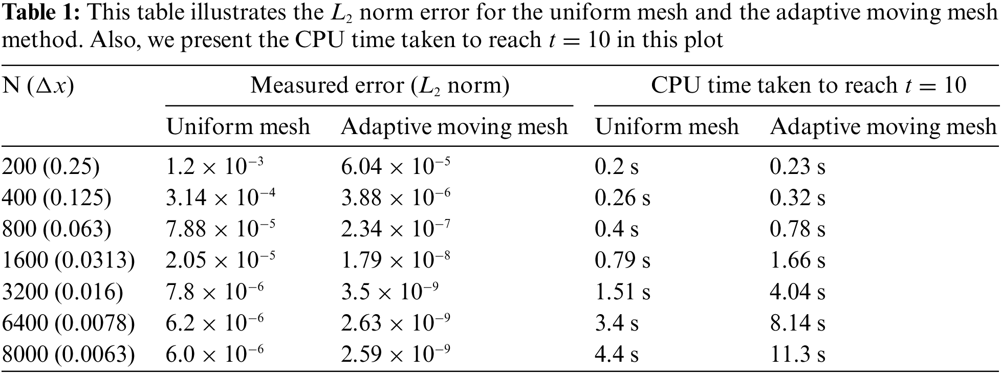
This figure shows the propagation and evolution of a nonlinear dispersive soliton wave, which is presented in the form of a bell-shaped profile, to Eq. (18). This wave arises in shallow water. The red spots in Fig. 2a manifest a magnificent number of mesh points that are nicely redistributed to the curvature ahead and behind it. The crucial idea of the adaptive moving mesh method is that this method feeds the curvature regions with more and more points. As a result, the error decreased to be acceptable, as can be seen in Fig. 5. Table 1 presents how the numerical results converge to the exact solution and the CPU time consumed for both uniform and adaptive moving mesh schemes. In Table 1, we can observe that the adaptive method provides significant results compared with the uniform mesh method. For instance, the L2 norm error reaches 1.2×10−3 when we use a uniform mesh while it reduces to 6.04×10−5 when we use the adaptive method at N=200. When we increase the number of the points the error decreases for both methods. However, it becomes smaller for the adaptive method. For example, the L2 norm error arrives at 6.0×10−6 for the uniform mesh and stands at 2.59×10−9 for the adaptive moving mesh method at N=8000. The adaptive technique consumes more CPU time than the uniform mesh method. In conclusion, we can safely say that the adaptive scheme is more accurate and reliable compared to the uniform mesh method.

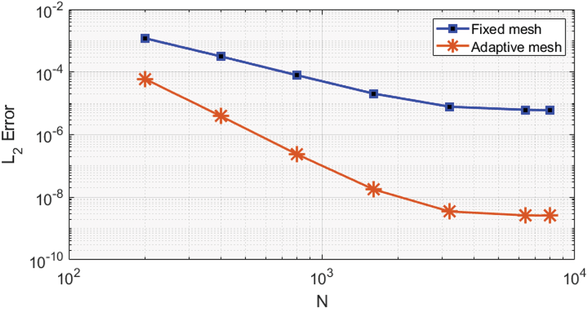
Figure 5: The L2 error resulting from using the fixed mesh and the adaptive mesh is shown in this figure. The parameter values are taken by k=0.5, w=4/3, a=−20, b=30, N=1000, τ=10−4, α=10 at time t=10.

6  Conclusions

In this work, we have used the generalized algebraic method, Jacobi’s elliptic functions approach, and the improved Q-expansion technique to produce some traveling wave solutions to Eq. (2) in terms of trigonometric and hyperbolic functions. We have also used the adaptive moving mesh method to generate the numerical solutions for the proposed problem. We noticed that the methods used provide better results than other methods, such as the cosine function method. Eq. (2) has been the subject of the previous studies presented in the literature review, which have mostly concentrated on establishing the numerical solutions rather than attempting to minimize the resultant error. However, this study obtained the numerical solutions and reduced the error. Compared to the methods using a uniform mesh, the adaptive approach is more dependable. Our findings also indicate that the adaptive mesh approach distributes the points in the high-error region. As a result, the L2 norm error decreases as the number of points increases. Furthermore, some 2D and 3D figures have been successfully drawn to show the efficacy of the approaches used. For instance, Fig. 2a demonstrates that the numerical solution of the proposed problem is greatly compatible with its exact solution. This provides a powerful evidence on how accurately the employed procedures perform. The exact and numerical approaches used are useful, efficient, and adaptable for generating certain types of traveling wave solutions for nonlinear PDEs.

Acknowledgement: The authors wish to express their appreciation to the reviewers for their helpful suggestions which greatly improved the presentation of this paper.

Funding Statement: The authors received no specific funding for this study.

Conflicts of Interest: The authors declare that they have no conflicts of interest to report regarding the present study.

References

1. Chen, G., Xin, X., Liu, H. (2019). The improved exp(−ϕ(η))-expansion method and exact solutions of nonlinear evolution equations in mathematical physics. Advances in Mathematical Physics, 2019(9), 4354310–4354318. https://doi.org/10.1155/2019/4354310 [Google Scholar] [CrossRef]
2. Kumar, D., Seadawy, A., Joardar, A. (2018). Modified Kudryashov method via exact solutions for some conformable fractional differential equations arising in mathematical biology. Chinese Journal of Physics, 56(1), 75–85. https://doi.org/10.1016/j.cjph.2017.11.020 [Google Scholar] [CrossRef]
3. Bekir, A., Unsal, O. (2012). Analytic treatment of nonlinear evolution equations using first integral method. Pramana Journal Physics, 79(1), 3–17. https://doi.org/10.1007/s12043-012-0282-9 [Google Scholar] [CrossRef]
4. Bai, C., Jie, C., Zhao, H. (2005). A new generalized algebraic method and its application in nonlinear evolution equations with variable coefficients. Zeitschrift für Naturforschung A, 60(4), 211–220. https://doi.org/10.1515/zna-2005-0401 [Google Scholar] [CrossRef]
5. Aasaraai, A. (2015). The application of modified F-expansion method solving the maccari’s system. Advances in Mathematics and Computer Science, 11(5), 1–14. https://doi.org/10.9734/BJMCS/2015/19938 [Google Scholar] [CrossRef]
6. Liu, S., Fu, Z., Liu, S., Zhao, Q. (2001). Jacobi elliptic function expansion method and periodic wave solutions of nonlinear wave equations. Physics Letters A, 289(1), 69–74. https://doi.org/10.1016/S0375-9601(01)00580-1 [Google Scholar] [CrossRef]
7. Alharbi, A., Almatrafi, M. (2020). Analytical and numerical solutions for the variant Boussinseq equations. Journal of Taibah University for Science, 14(1), 454–462. https://doi.org/10.1080/16583655.2020.1746575 [Google Scholar] [CrossRef]
8. Alharbi, A., Almatrafi, M. (2020). Numerical investigation of the dispersive long wave equation using an adaptive moving mesh method and its stability. Results in Physics, 16(9), 102870. https://doi.org/10.1016/j.rinp.2019.102870 [Google Scholar] [CrossRef]
9. Alharbi, A., Almatrafi, M. (2020). Riccati-Bernoulli Sub-ODE approach on the partial differential equations and applications. International Journal of Mathematics and Computer Science, 15(1), 367–388. [Google Scholar]
10. Alharbi, A., Almatrafi, M. (2020). New exact and numerical solutions with their stability for Ito integro-differential equation via Riccati-Bernoulli sub-ODE method. Journal of Taibah University for Science, 14(1), 1447–1456. https://doi.org/10.1080/16583655.2020.1827853 [Google Scholar] [CrossRef]
11. Alharbi, A., Almatrafi, M. (2020). Exact and numerical solitary wave structures to the variant boussinesq system. Symmetry, 12(9), 1473. https://doi.org/10.3390/sym12091473 [Google Scholar] [CrossRef]
12. Almatrafi, M., Alharbi, A., Tunç, C. (2020). Constructions of the soliton solutions to the good Boussinesq equation. Advances in Continuous and Discrete Models, 629. https://doi.org/10.1186/s13662-020-03089-8 [Google Scholar] [CrossRef]
13. Alharbi, A., Almatrafi, M., Seadawy, A. (2020). Construction of the numerical and analytical wave solutions of the Joseph-Egri dynamical equation for the long waves in nonlinear dispersive systems. International Journal of Modern Physics B, 34(30), 2050289. https://doi.org/10.1142/S0217979220502896 [Google Scholar] [CrossRef]
14. Alharbi, A., Almatrafi, M., Lotfy, K. (2020). Constructions of solitary travelling wave solutions for Ito integro-differential equation arising in plasma physics. Results in Physics, 19(1), 103533. https://doi.org/10.1016/j.rinp.2020.103533 [Google Scholar] [CrossRef]
15. Akinyemi, L., Şenol, M., Az-Zo’bi, E., Veeresha, P., Akpan, U. (2022). Novel soliton solutions of four sets of generalized (2+1)-dimensional Boussinesq-Kadomtsev-Petviashvili-like equations. Modern Physics Letters B, 36(1), 2150530. https://doi.org/10.1142/S0217984921505308 [Google Scholar] [CrossRef]
16. Akinyemi, L., Morazara, E. (2023). Integrability, multi-solitons, breathers, lumps and wave interactions for generalized extended Kadomtsev-Petviashvili equation. Nonlinear Dynamics, 111, 4683–4707. https://doi.org/10.1007/s11071-022-08087-x [Google Scholar] [CrossRef]
17. Al-Mamun, A., Ananna, S., Gharami, P., An, T., Asaduzzaman, M. (2022). The improved modified extended tanh-function method to develop the exact travelling wave solutions of a family of 3D fractional WBBM equations. Results in Physics, 41(2–3), 105969. https://doi.org/10.1016/j.rinp.2022.105969 [Google Scholar] [CrossRef]
18. Al-Mamun, A., Ananna, S., An, T., Asaduzzaman, M., Rana, M. (2022). Sine-gordon expansion method to construct the solitary wave solutions of a family of 3D fractional WBBM equations. Results in Physics, 40(2–3), 105845. https://doi.org/10.1016/j.rinp.2022.105845 [Google Scholar] [CrossRef]
19. Benjamin, T., Bona, J., Mahony, J. (1972). Model equations for long waves in non-linear dispersive systems. Philosophical Transactions of the Royal Society of London. Series A, Mathematical and Physical Sciences, 272(1220), 47–78. https://doi.org/10.1098/rsta.1972.0032 [Google Scholar] [CrossRef]
20. Peregrine, D. (1966). Calculations of the development of an undular bore. Journal of Fluid Mechanics, 25(2), 321–330. https://doi.org/10.1017/S0022112066001678 [Google Scholar] [CrossRef]
21. Bulut, H., Sulaiman, T., Baskonus, H. (2017). On the new soliton and optical wave structures to some nonlinear evolution equations. The European Physical Journal Plus, 132(11), 459. https://doi.org/10.1140/epjp/i2017-11738-7 [Google Scholar] [CrossRef]
22. Pervin, S., Habib, M. (2020). Solitary wave solutions to the Korteweg-de Vries (KdV) and the Modified Regularized Long Wave (MRLW) equations. International Journal of Mathematics and its Applications, 8(1), 1–5. [Google Scholar]
23. Khalifa, A., Raslan, K., Alzubaidi, H. (2008). A collocation method with cubic B-splines for solving the MRLW equation. Journal of Computational and Applied Mathematics, 212(2), 406–418. https://doi.org/10.1016/j.cam.2006.12.029 [Google Scholar] [CrossRef]
24. Karakoc, G., Geyikli, T. (2013). Petrov-Galerkin finite element method for solving the MRLW equation. Mathematical Sciences, 7(1), 25. https://doi.org/10.1186/2251-7456-7-25 [Google Scholar] [CrossRef]
25. Haq, F., Islam, S., Tirmizi, I. (2010). A numerical technique for solution of the MRLW equation using quartic B-splines. Applied Mathematical Modelling, 34(12), 4151–4160. https://doi.org/10.1016/j.apm.2010.04.012 [Google Scholar] [CrossRef]
26. Alharbi, A. (2023). Traveling-wave and numerical solutions to a Novikov-Veselov system via the modified mathematical methods. AIMS Mathematics, 8(1), 1230–1250. https://doi.org/10.3934/math.2023062 [Google Scholar] [CrossRef]
27. Jena, S., Senapati, A., Gebremedhin, G. (2020). Approximate solution of MRLW equation in B-spline environment. Mathematical Sciences, 14(4), 345–357. https://doi.org/10.1007/s40096-020-00345-6 [Google Scholar] [CrossRef]
28. Raslan, K., Hassan, S. (2009). Solitary waves for the MRLW equation. Applied Mathematics Letters, 22(7), 984–989. https://doi.org/10.1016/j.aml.2009.01.020 [Google Scholar] [CrossRef]
29. Khan, Y., Taghipour, R., Falahian, M., Nikkar, A. (2013). A new approach to modified regularized long wave equation. Neural Computing and Applications, 23(5), 1335–1341. https://doi.org/10.1007/s00521-012-1077-0 [Google Scholar] [CrossRef]
30. Karakoç, S., Ak, T., Zeybek, H. (2014). An efficient approach to numerical study of the MRLW equation with B-spline collocation method. Abstract and Applied Analysis, 2014(2), 596406. https://doi.org/10.1155/2014/596406 [Google Scholar] [CrossRef]
31. Essa, Y., Abouefarag, I., Rahmo, E. (2014). The numerical solution of the MRLW equation using the multigrid method. Applied Mathematics, 21(5), 3328–3334. https://doi.org/10.4236/am.2014.521310 [Google Scholar] [CrossRef]
32. Zhang, S., Li, J., Zhou, Y. (2015). Exact solutions of non-linear lattice equations by an improved Exp-function method. Entropy, 17(5), 3182–3193. https://doi.org/10.3390/e17053182 [Google Scholar] [CrossRef]
33. Alharbi, A., Naire, S. (2017). An adaptive moving mesh method for thin film flow equations with surface tension. Journal of Computational and Applied Mathematics, 319(4), 365–384. https://doi.org/10.1016/j.cam.2017.01.019 [Google Scholar] [CrossRef]
34. Budd, C., Huang, W., Russell, R. (2009). Adaptivity with moving grids. Acta Numerica, 18, 111–241. https://doi.org/10.1017/S0962492906400015 [Google Scholar] [CrossRef]
35. Alharbi, A., Naire, S. (2019). An adaptive moving mesh method for two-dimensional thin film flow equations with surface tension. Journal of Computational and Applied Mathematics, 356(3), 219–230. https://doi.org/10.1016/j.cam.2019.02.010 [Google Scholar] [CrossRef]
36. Huang, W., Russell, R. (2011). The adaptive moving mesh methods. New York, NY: Springer. https://doi.org/10.1007/978-1-4419-7916-2 [Google Scholar] [CrossRef]
37. Alharbi, A. (2016). Numerical solution of thin-film flow equations using adaptive moving mesh methods (Ph.D. Thesis). Keele University. https://eprints.keele.ac.uk/id/eprint/2356 [Google Scholar]
Cite This Article
Copyright © 2023 The Author(s). Published by Tech Science Press.
This work is licensed under a Creative Commons Attribution 4.0 International License , which permits unrestricted use, distribution, and reproduction in any medium, provided the original work is properly cited.
Downloads
Citation Tools