Fine-Grained Point Cloud Intensity Correction Modeling Method Based on Mobile Laser Scanning

1  Introduction

Over the past three decades, Light Detection and Ranging (LiDAR) technology has demonstrated broad application prospects across diverse domains, including remote sensing science [1], autonomous driving [2], environmental monitoring [3], forestry [4,5], engineering surveying [6], and the Internet of Things [7,8], due to its high precision and non-contact measurement characteristics. This technology reconstructs the three-dimensional morphology of target objects by emitting laser pulses and receiving reflected signals, while simultaneously recording the laser reflection intensity information. As a critical complement to point cloud three-dimensional geometric data, intensity reflects the reflective spectral characteristics of the scanning object at specific locations, serving as a pivotal parameter for object recognition and detection [9–13].

However, the intensity data acquired by LiDAR systems are subject to systematic distortions caused by a complex interplay of multiple influencing factors. These include sensor inherent properties, target surface physical characteristics, environmental conditions, and data acquisition geometry. These distortions result in significant deviations from the true reflectance properties of scanned surfaces. Among these factors, distance and incidence angle, exert particularly pronounced impacts on intensity information [14,15]. To reduce the impact of these two factors on intensity, researchers have proposed various correction strategies, mainly divided into model-driven methods [16–18] and data-driven methods [19–21].

Model-driven methods build physical mathematical models based on the laser ranging equation and theoretically have the capability for high-precision correction. However, in practical applications, these methods encounter several limitations, including intricate parameter optimization requirements, computationally intensive processing procedures, and constrained model generalizability. These challenges significantly hinder their effectiveness and adaptability in complex real-world applications. Data-driven methods in LiDAR intensity estimation, like other artificial intelligence (AI) models [22–25], depend on extensive training data. They utilize polynomial regression models to correct intensity deviations. These methods provide enhanced applicability and practicality. They are particularly effective in complex scenarios with partially unknown LiDAR parameter information.

While data-driven methods offer substantial advantages, the prevailing modeling methodologies predominantly rely on Terrestrial Laser Scanning (TLS) technology [26,27]. These techniques have partially addressed the challenges related to the efficiency and accuracy of data acquisition required for constructing intensity correction models. The TLS methodology necessitates the establishment of discrete sampling stations for data collection. Each individual sampling station is constrained to generating a restricted dataset of distance-intensity or incidence angle-intensity measurements. Furthermore, this approach requires recurrent manual repositioning of the LiDAR instrument relative to the target object to satisfy the uniformity criteria essential for effective model construction. This process is not only time-consuming and labor-intensive but also prone to manual error to degrade the accuracy of modeling.

In the acquisition of distance-intensity data with identical incidence angle values, researchers commonly need to manually ensure that the angle between the LiDAR scanning centerline and the diffuse reflector remains constant in order to meet the experimental condition of incidence angle consistency. For example, Xu et al. [28] and Tan et al. [29] placed the LiDAR directly facing the diffuse reflector to set the incidence angle at 0°, thereby minimizing the impact of the incidence angle on intensity measurements. However, in practical scenarios, slight tilting of the diffuse reflector’s surface can disrupt the consistency of the incidence angle, adversely influencing the model’s accuracy. To tackle this problem, Li et al. [21] proposed an incidence angle calculation method based on plane fitting. Although this method theoretically enhances the precision of incidence angle measurement, it still necessitates manual configuration to ensure that the incidence angle values at each distance station are maintained within a small error range when acquiring intensity data solely related to distance factors. This process requires multiple station adjustments in practice, thereby increasing the complexity and time cost of the experiments.

Similarly, when exploring the impact of the incidence angle on intensity values, researchers typically employ manual operations to maintain a constant distance between the LiDAR scanning centerline and the central axis of the diffuse reflector, thereby satisfying the experimental condition of distance consistency. For example, Tan et al. [29] fixed the distance between the LiDAR and the central axis of the diffuse reflector and rotated the reflector at 10° intervals to obtain different incidence angle-intensity data at the same distance value. However, in practice, minor deviations in the distance value can significantly impact modeling accuracy. To address this issue, Bolkas [30] proposed a method involving a fan-shaped arrangement of diffuse reflectors. Within the incidence angle range of 0° to 80°, they manually set up stations to ensure that the reflectors were distributed at a fixed distance from the LiDAR emitter. Although this method enhances experimental controllability to some extent, it imposes extremely high requirements for precise positioning of the diffuse reflectors, necessitating great caution during practical implementation. In light of the limitations of existing TLS modeling methods, exploring a more precise and automated data acquisition method that reduces human intervention has become a key direction for improving model accuracy.

The development of Mobile Laser Scanning (MLS) technology provides a new approach to solving this problem [31–34]. In comparison to TLS, MLS technology does not only maintain measurement precision but also significantly enhances the efficiency of data acquisition. It captures a vast array of point cloud data across diverse distances and incidence angles through continuous scanning for modeling purposes. A pivotal advantage of MLS lies in its ability to automatically retrieve and compute the distance, incidence angle, and intensity information for each measurement point utilizing a grid index structure [35]. This process facilitates the selection of high-precision modeling samples that adhere to consistency conditions without the necessity for manual intervention. Consequently, the utilization of the MLS method for data acquisition effectively circumvents errors associated with manual operations, thereby ensuring the procurement of modeling samples with superior accuracy.

Therefore, this study proposes a fine-grained point cloud intensity correction modeling method based on MLS technology. The method leverages the continuous scanning advantage of MLS to collect point cloud intensity of standard diffuse reflector plates at various distances and incidence angles, obtaining a rich dataset. Then, a fine-grained screening strategy is used to accurately screen a large number of distance-intensity and incidence angle-intensity samples for modeling. Finally, a high-precision intensity correction model is established based on the screened sample data. The experimental results demonstrate that the proposed modeling method in this study is characterized by a high degree of automation and the accuracy of the modeling data. It does not only address the issue of low modeling efficiency associated with existing TLS methods but also significantly enhances the precision of the modeling data, thereby effectively improving the consistency of the corrected intensity.

The structure of this paper is organized as follows: Section 2 elaborates on the theoretical foundation for establishing the intensity correction model, detailing the methodological processes including the acquisition and organization of MLS point cloud data, the construction of the training dataset, and the testing of the correction model, in conjunction with the experimental materials. Section 3 validates the efficacy and precision of the MLS modeling approach through the analysis of experimental results, providing a comparative assessment against the conventional TLS modeling method. Conclusively, Section 4 summarizes the principal contributions of this research and outlines prospective directions for future investigation.

2  Materials and Methods

The proposed methodology is delineated into three sequential steps: dataset construction, intensity correction model establishment, and model testing. The overarching workflow of the research methodology is illustrated in Fig. 1.

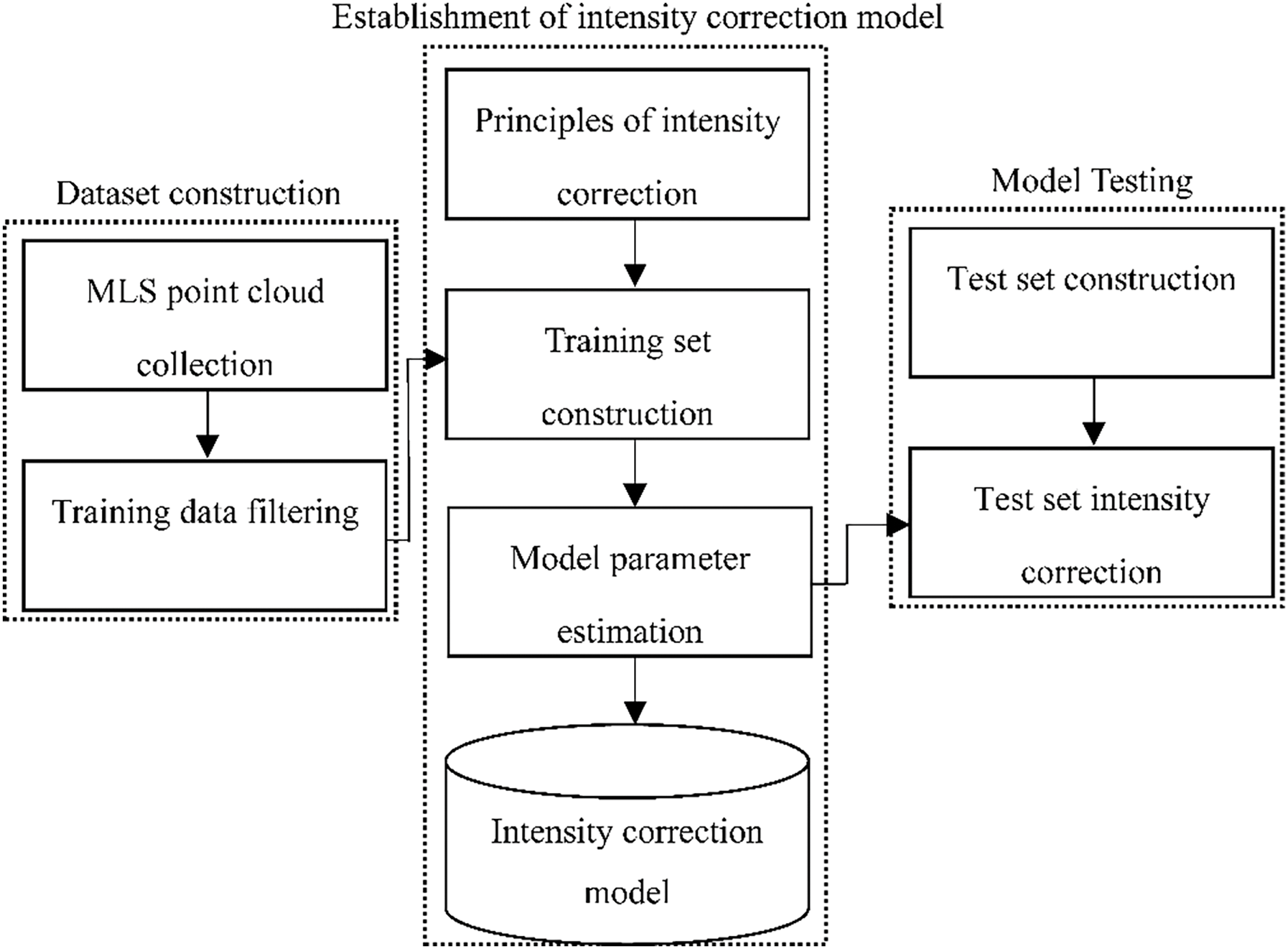
Figure 1: Flowchart of research method

This study employs a systematic methodology to construct and validate an intensity correction model based on MLS technology. During the dataset construction phase, a UTM-30LX 2D LiDAR was utilized, with a standard diffuse reflector exhibiting 50% reflectivity serving as the target for point cloud data acquisition. To ensure the quality of the training data, a rigorous fine-grained filtering strategy was implemented to extract representative distance-intensity and incidence angle-intensity training samples from the raw point cloud data. In the correction model construction phase, the study first conducted a systematic analysis of the key factors influencing MLS point cloud intensity measurements, thereby establishing a multiplicative model-based intensity correction framework. Subsequently, polynomial regression was applied to fit the training dataset, with model parameters estimated using the least squares method, culminating in the development of a comprehensive intensity correction model. To validate the effectiveness and robustness of the proposed method, an independent test dataset was constructed for model evaluation. By applying the intensity correction model to this test dataset and quantitatively comparing the results with intensity information corrected using traditional TLS modeling methods, the performance of the proposed modeling approach was systematically evaluated.

2.1 Intensity Correction Model

2.1.1 Intensity Correction Principle

In the LiDAR system, the received laser power is related to multiple parameters, including the transmitted laser power , the atmospheric transmission coefficient , the receiving aperture size of the LiDAR, the transmission coefficient of the LiDAR optical system, the scanning distance , the incidence angle , and the target reflectivity . Based on the laser ranging equation [20], when the target surface follows Lambertian reflection characteristics, the relationship between and these parameters can be simplified as:

(1)

For a specific LiDAR system, , , , and are relatively stable and can be regarded as constants. Therefore, is mainly affected by , , and . Since is linearly related to the intensity data, the main influencing factors of the intensity are also these three parameters. Research has shown that, assuming the independence of factors influencing intensity, a multiplicative model can be applied to quantify the relationships between variables [14,26]. The relationship is described as follows:

(2)

where represents the original intensity value obtained for an object target with reflectivity at and . , , and respectively represent the functional relationships between the original intensity value and , , and .

For a scanned object with a fixed reflectivity , the theoretical intensity value at the reference distance and the reference incidence angle can be expressed as:

(3)

By combining Eqs. (2) and (3) to eliminate , the transformation relationship between the original intensity value and the theoretical intensity value under the reference condition can be obtained, that is:

(4)

This relationship constitutes the basic framework of the correction model. After determining the specific functional forms of and , the original intensity data can be corrected accordingly to obtain the theoretical intensity value that is only related to the target reflectivity .

2.1.2 Model Parameter Estimation

To obtain a function that reflects the relationship between distance and intensity as a single variable, for scanning objects with a fixed reflectance value, the incidence angle is kept constant to obtain intensity data at different distances. Since the obtained distance-intensity data pairs are distributed within a definite closed interval, according to the Weierstrass Approximation Theorem [36], a polynomial function can be used to fit their relationship. Additionally, considering that LiDAR intensity data exhibits a trend of increasing and then decreasing with distance within a certain range, this study ultimately chooses a piecewise polynomial function for fitting, with the specific expression as follows:

(5)

where represents the function fitted from distance-intensity modeling samples, and are the degrees of the fitting polynomials for the closer and farther distance segments, respectively, and and are the corresponding polynomial coefficients.

The values of and can be determined by comparing the fitting accuracy of polynomials of different degrees. The specific parameters and can be calculated using the method of least squares. The boundary point is typically set at the intensity peak [21]. This boundary point serves as a critical threshold for segmenting the distance into closer and farther regions, ensuring that each divided distance interval maintains a consistent intensity variation trend within its respective range. To obtain a function that reflects the relationship between distance and intensity as a single variable, for scanning objects with a fixed reflectance value, the distance value is kept constant to obtain intensity data at different incidence angles. Similarly, for the obtained incidence angle-intensity data pairs, the Weierstrass Approximation Theorem allows the use of a cosine polynomial model for fitting, with the specific expression as follows:

(6)

where represents the function fitted from incidence angle-intensity modeling samples, is the degree of the cosine polynomial, and are the corresponding polynomial coefficients. The value of is also determined by comparing the fitting accuracy of polynomials of different degrees. The specific parameters are calculated using the method of least squares.

2.2 MLS Measurement System

2.2.1 Hardware Components

In this paper, an MLS measurement system based on 2D LiDAR is independently designed to collect point cloud data of the standard diffuse reflector plate at different distances and incidence angles. The detailed configuration of this system is shown in Fig. 2.

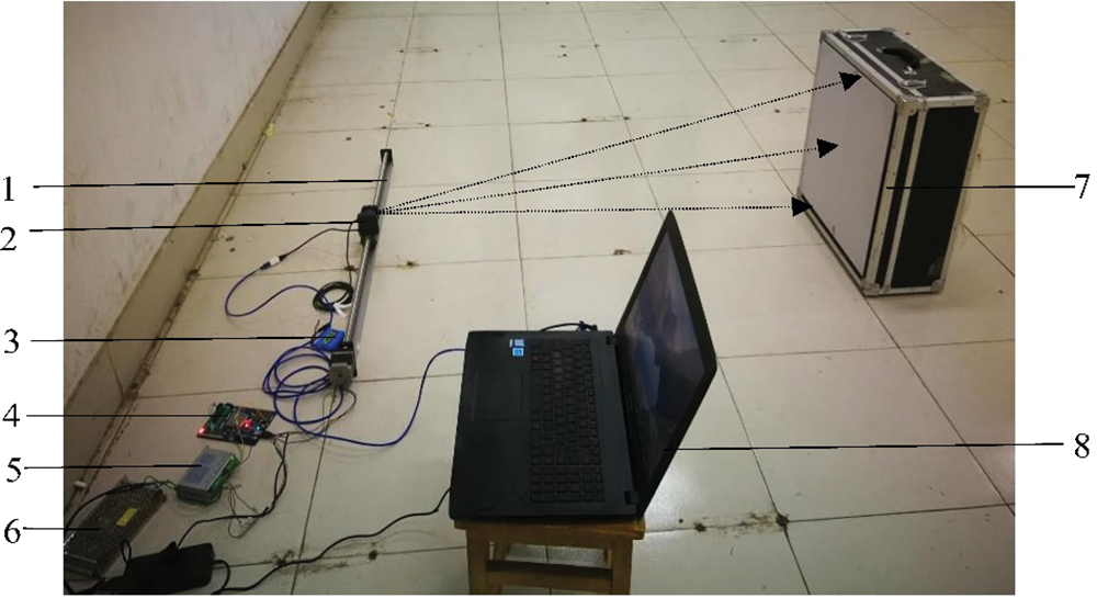
Figure 2: Configuration of MLS measurement system. 1. Linear guide slide module 2. UTM-30LX-EW 2D LiDAR 3. LiDAR power supply 4. Microcontroller 5. Hybrid stepper motor driver 6. 12 V switching power supply 7. Scanned object 8. Portable computer

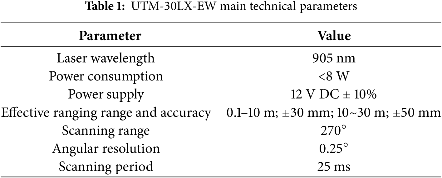
The core components of the MLS measurement system include: a 2D LiDAR sensor (UTM-30LX-EW, Hokuyo, Japan), a linear guide slide module (FLS40L100010C7, FUYU, China), a hybrid stepper motor driver (57HBP112AL4, EASTOUR, China), a microcontroller (STC89C52, STC, China), and a portable computer (S14UA8250, ASUS, China). Among them, the 2D LiDAR sensor of the model UTM-30LX-EW has a laser wavelength of 905 nm, a maximum ranging capability of 30 m, and a wide field of view of 270°, which can meet the measurement requirements in different scenarios. In terms of ranging accuracy, the LiDAR sensor achieves an accuracy of ±30 mm within the range of 0.1 to 10 m, and ±50 mm within the range of 10 to 30 m. In addition, its angular resolution is 0.25°, and the scanning period is only 25 ms. A single scan can capture up to 1081 data points, with high acquisition efficiency and sampling density. Its main technical parameters are shown in Table 1.

During data acquisition, the 2D LiDAR sensor is laterally installed on the guide slide to ensure that the scanning area completely covers the target object. A standard diffuse reflector plate with a size of 50 cm × 50 cm and a reflectivity of 50% is selected as the reference target. The diffuse reflector plate is placed directly opposite the fan-shaped scanning area of the LiDAR to obtain the best measurement effect. After the system is started, the microcontroller runs and drives the slide to move smoothly at a preset constant speed of 0.01 m/s by precisely controlling the stepper motor driver. During this process, the 2D LiDAR sensor transmits the real-time scanning data to the portable computer through the integrated network interface and stores it in the. DAT format for subsequent data processing and analysis.

Compared to the conventional TLS modeling approach, the experimental apparatus designed in this study demonstrates significant advantages. Firstly, the lateral installation of the 2D LiDAR sensor enables continuous scanning, effectively eliminating artificial errors associated with frequent device adjustments in traditional discrete sampling methods. Secondly, the integration of a high-precision linear guide rail with a stepper motor drive system ensures both smooth sensor movement and precise speed control, thereby substantially reducing data errors caused by motion instability. The developed MLS measurement system exhibits superior data acquisition speed and measurement accuracy, providing a more reliable and efficient experimental methodology for LiDAR intensity calibration research.

2.2.2 Point Cloud Coordinate Calculation

In this study, a two-dimensional grid index structure is adopted to organize and manage the point cloud data acquired by the MLS measurement system. Each measurement point is uniquely identified according to its frame number and in-frame number for easy subsequent data retrieval. To visually display the point cloud data collected in the distance and incidence angle experiments, a global coordinate system is established with the initial position of the 2D LiDAR on the moving slide as the reference, and its structure is shown in Fig. 3.

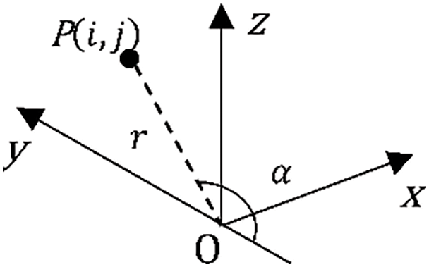
Figure 3: Coordinate system of point cloud

Among them, the -axis is along the moving forward direction of the slide, the -axis points in the horizontal scanning direction of the 2D LiDAR, and the -axis extends vertically upward. Based on this coordinate system, the three-dimensional coordinates of the measurement point can be accurately calculated by the following formulas:

(7)

where is the moving speed of the slide, is the LiDAR scanning period, is the LiDAR scanning angle, and is the actual distance from the LiDAR laser transmitter to the scanning point.

2.3 Data Set Construction

2.3.1 Site Layout

In this study, distance and incidence angle experiments are designed under strictly controlled indoor environmental variables. In the distance experiment, the diffuse reflector plate at each site is placed perpendicular to the horizontal plane and directly facing the 2D LiDAR scanning center line to minimize the fluctuation range of the incidence angle, approaching 0°. According to the characteristics of the UTM-30LX-EW sensor, the intensity data fluctuates greatly at a short distance and tends to be stable at a long distance. To avoid data uncertainty and accuracy loss at extremely close or relatively long distances, the experiment selects to set sites within the short-distance range where the intensity data fluctuates most significantly to evaluate the distance correction performance of the proposed modeling method. Specifically, the distance experiment uniformly arranges 30 sites within the range of 0.1 to 3.0 m at an interval of 0.1 m.

In the incidence angle experiment, the diffuse reflector plate is fixed at a distance of 1.0 m from the 2D LiDAR scanning center line, and the incidence angle sites are set by adjusting the angle between it and the LiDAR scanning plane. Considering that the intensity data of the UTM-30LX-EW sensor decreases significantly with the increase of the incidence angle within the range of 0° to 80° and the measurement accuracy is relatively high, while the error is relatively large when the incidence angle value exceeds 80°. Therefore, 9 sites are uniformly set at an interval of 10° within the range of 0° to 80° to evaluate the incidence angle correction performance of the proposed modeling method.

Fig. 4a,b visually shows the relative position relationship between the diffuse reflector plate and the MLS measurement system at different sites in the distance and incidence angle experiments.

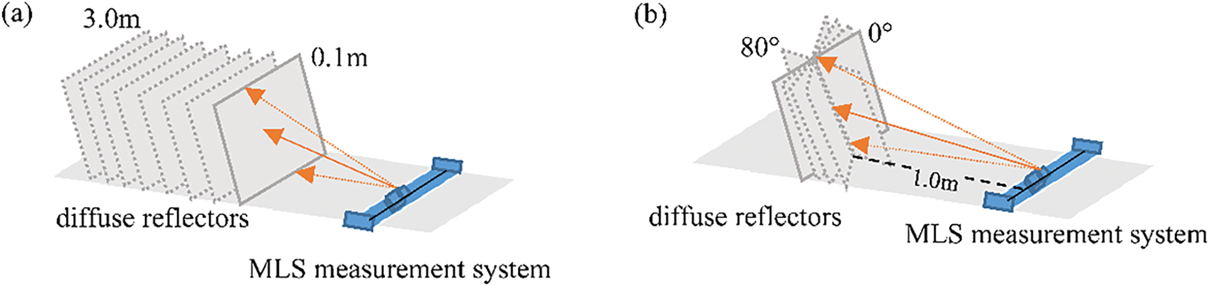
Figure 4: Relative position relationship between diffuse reflectors and MLS measurement system at different stations in distance and incidence angle experiments. (a) The position relationship between diffuse reflectors and MLS measurement system in distance experiments; (b) The position relationship between diffuse reflectors and MLS measurement system in the incidence angle experiment

To ensure the effectiveness of the data set, this study performs Region of Interest (ROI) region screening and preprocessing operations on the point cloud data collected at all sites. First, the coordinate range of the diffuse reflector plate is determined according to the preset position information. Then, based on these coordinate ranges, the point cloud points near the edge of the diffuse reflector plate within 5 cm are removed to effectively reduce the interference of noise data. After the above preprocessing steps, the ROI region of the diffuse reflector plate is successfully screened.

2.3.2 Point Cloud Incidence Angle Calculation

In this study, a method based on a spherical neighborhood fitting plane [29] is adopted to calculate the incidence angle of each measurement point in the ROI region point cloud. The core of this method is to determine the angle between the LiDAR emission beam and the normal of the scanned target surface at the point . Fig. 5 shows in detail the geometric principle of the incidence angle calculation.

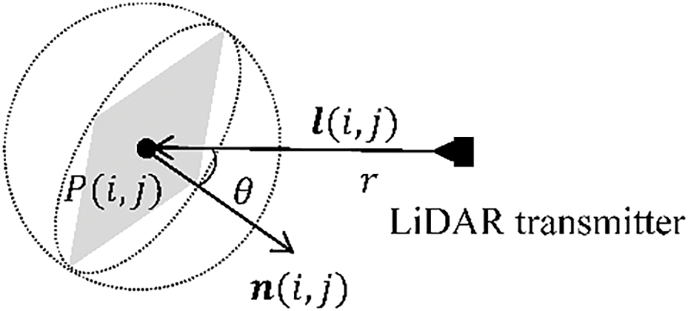
Figure 5: Geometric principle of incidence angle calculation

Specifically, the vector represents the incidence laser direction from the LiDAR transmitter to the measurement point on the object surface, and its direction and magnitude are jointly determined by the three-dimensional coordinates of the LiDAR transmitter and the point , with a value of . represents the normal direction of the fitting plane of all neighboring points within the local spherical neighborhood of the measurement point .The value of can be determined through least squares fitting, which provides an optimal solution by minimizing the sum of squared residuals between the observed points and the fitted plane [29,37]. On this basis, the cosine value of the incidence angle can be accurately calculated by the following formula:

(8)

where “” represents the dot product operation of two vectors, and |||| represents the vector norm operation.

In terms of the selection of the neighborhood radius size, considering that the short-distance ranging accuracy of the UTM-30LX-EW sensor is ±30 mm, this accuracy characteristic significantly affects the point cloud distribution. If the neighborhood radius is less than the accuracy threshold, the fitting plane may deviate from the expected XOZ plane direction and tend to the YOZ plane direction, which will cause a large error in the incidence angle calculation. To avoid this situation, the neighborhood radius is set to 30 mm. Based on the setting of this neighborhood radius, this study conducted a comprehensive analysis of the resolution in both the mobile slider’s forward direction and the LiDAR scanning direction. This analysis aims to evaluate whether sufficient neighboring points are contained within the neighborhood of measurement point for effective plane fitting. The resolution calculations for both the mobile slider’s forward direction and the LiDAR scanning direction are expressed through the following formulas:

(9)

where represents the resolution in the mobile slider’s forward direction, and denotes the resolution in the LiDAR scanning direction.

In the forward direction of the mobile slider, since the slide speed is 0.01 m/s and the scanning period is 25 ms, the calculated resolution is 2.5 mm. Consequently, with a neighborhood radius of 30 mm, the forward direction contains a minimum of 24 points. Regarding the LiDAR scanning direction, the scanning angle resolution is 0.25°, yields a spatial resolution that remains below 13 mm within a distance value of 3.0 m. Therefore, with the same 30 mm neighborhood radius, the scanning direction encompasses at least 4 points. In conclusion, the neighborhood radius of 30 mm ensures a sufficient number of points within the neighborhood of measurement point to satisfy the requirements for robust plane fitting.

2.3.3 Training Data Screening

To select the modeling samples that reflect the single-variable relationships between distance and intensity and between incidence angle and intensity from the acquired point cloud, a fine-grained screening strategy is adopted in this study.

When selecting the distance-intensity modeling samples, first, the screening condition for the incidence angle is set to be between 0° and 0.1° to ensure the consistency of the incidence angle. Then, according to the established index structure, all the measurement points that meet the screening conditions are accurately extracted from the point cloud obtained in the distance experiment. On this basis, the distance and intensity values of these measurement points are statistically analyzed to generate representative distance-intensity modeling samples.

The selection process of the incidence angle-intensity modeling samples is similar to the above, but the screening conditions are different. First, the distance screening condition is set to 1.000 m to ensure the consistency of the distance value. Then, by using the two-dimensional grid index, all the measurement points that meet the screening conditions are extracted from the point cloud obtained in the incidence angle experiment. Finally, the incidence angle and intensity values of these measurement points are statistically analyzed to produce valid incidence angle-intensity modeling samples.

2.4 Model Testing

2.4.1 Test Set Construction

To evaluate the performance of the proposed MLS modeling method in distance and incidence angle correction, this study constructs two independent test sets. Specifically, by using the established two-dimensional grid index, the ROI area obtained in Section 2.3.1 is filtered, retaining only the data that did not participate in the model training as the test set, ensuring the complete independence of the test set from the training data. The construction of the test set is divided into two parts: Test Set 1 is derived from the data selection of the distance experiment, characterized by a wide range of distance variations and a relatively narrow range of incidence angle variations. Test Set 2 is derived from the data selection of the incidence angle experiment, featuring a broad range of incidence angle variations and a relatively limited range of distance variations.

2.4.2 Intensity Correction

For the test set data, the established model is applied for intensity correction processing. The correction steps are as follows: First, set the reference distance = 1.0 m and the reference incidence angle = 0° as the correction benchmark. Then, according to the method described in Section 2.3.2, accurately calculate the cosine value of the incidence angle for each measurement point , and directly obtain the distance value and the original intensity value at that measurement point through the two-dimensional grid index. Next, substitute the , , and at each measurement point into the Eq. (4) in Section 2.1.1, and combine the specific expressions of the distance piecewise polynomial and the incidence angle cosine polynomial determined in Section 2.1.2 to calculate the corrected intensity . Finally, replace the original intensity value with the corrected intensity , completing the correction of the intensity data for all measurement points in the test set.

2.5 Evaluation Metrics

To effectively assess the performance of the modeling method proposed in this paper in terms of intensity data correction, this study employs three core evaluation metrics: Root Mean Square Error (RMSE), Coefficient of Variation (CV), and the variance mean ratio . The specific definitions of each metric are as follows:

1.   Root Mean Square Error (RMSE)

Root Mean Square Error is used to measure the fitting accuracy of the polynomial function for intensity data at different degrees. Its calculation formula is:

(10)

where represents in the distance-intensity relationship or in the incidence angle-intensity relationship, and is the number of samples. The smaller the RMSE value, the higher the degree of matching between the fitting function and the actual data, indicating that the model can more accurately capture the dependency between intensity and distance or intensity and incidence angle.

2.   Coefficient of Variation (CV)

The Coefficient of Variation is used to quantify the degree of dispersion of the intensity data before and after correction, i.e., intensity consistency. Its calculation formula is defined as:

(11)

where STD denotes the standard deviation of the intensity data, and Mean denotes the mean value of the intensity data. The smaller the CV value, the less variability in the intensity data, indicating higher intensity consistency.

3.   Variance Mean Ratio

The variance mean ratio is the ratio of the variability of the intensity data before and after correction, used to quantify the performance of the intensity correction model. Its calculation formula is:

(12)

where represents the coefficient of variation of the original intensity data, and represents the coefficient of variation of the corrected intensity data. When the value is less than 1, it indicates that the variability of the corrected intensity data is lower than that of the original intensity data, suggesting that the correction model can effectively reduce the dispersion of the intensity data. The closer the value is to 0, the better the performance of the correction model in improving the consistency of the intensity data.

3  Results and Discussion

3.1 Benchmark Method

To evaluate the performance of the MLS modeling method in intensity correction, an experiment comparing it with the traditional TLS modeling method was designed. The experiment also used the UTM-30LX-EW 2D LiDAR sensor and a standard diffuse reflector plate with a reflectivity of 50% to collect training data, and the sampling site settings referred to the research of Tan et al. [26]. The experimental steps are as follows:

First, to establish the relationship model between distance and intensity, 30 groups of distance sites were uniformly set at intervals of 0.1 m within the distance range of 0.1 to 3 m. During this process, the LiDAR sensor was fixed on a tripod and precisely adjusted to ensure that the scanning center beam was directly facing the diffuse reflector plate, and the incidence angle was constant at 0° to eliminate the influence of the incidence angle factor on the results. At each site, 10 groups of intensity data were continuously recorded and averaged to obtain the distance-intensity modeling samples.

Second, to establish the relationship model between the incidence angle and intensity, 9 groups of incidence angle sites were uniformly set at intervals of 10° within the incidence angle range of 0° to 80°. The distance between the LiDAR center beam and the diffuse reflector plate at all sites was set to 1.0 m. At each site, 10 groups of intensity data were also continuously recorded and averaged to obtain the incidence angle-intensity modeling samples. Fig. 6a,b shows the relative position relationship between the diffuse reflector plate and the LiDAR sensor at different sites under the TLS modeling method, where Fig. 6a shows the position relationship in the distance experiment, and Fig. 6b shows the position relationship in the incidence angle experiment.

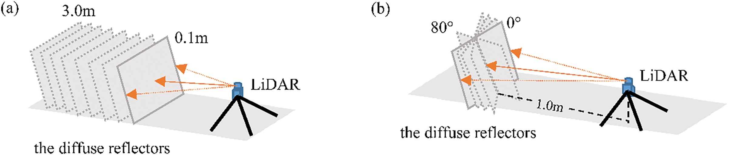
Figure 6: The relative position relationship between the diffuse reflectors and LiDAR at different stations under TLS modeling method. (a) The position relationship between the distance experiment diffuse reflectors and LiDAR; (b) The position relationship between diffuse reflector and LiDAR in incidence angle experiment

3.2 Training Results

3.2.1 Training Set

According to the training data screening method in Section 2.3.3, 13,671 groups of distance-intensity data pairs and 11,733 groups of incidence angle-intensity data pairs were collected. According to the TLS modeling comparison method in Section 3.1, only 30 groups of distance-intensity data pairs and 9 groups of incidence angle-intensity data pairs were obtained. Fig. 7a–d intuitively shows the distribution of the training data of distance and intensity and incidence angle and intensity obtained by the MLS and TLS modeling methods. Among them, Fig. 7a shows the distance and intensity training data of the MLS modeling method, Fig. 7b shows the incidence angle and intensity training data of the MLS modeling method, Fig. 7c shows the distance and intensity training data of the TLS modeling method, and Fig. 7d shows the incidence angle and intensity training data of the TLS modeling method.

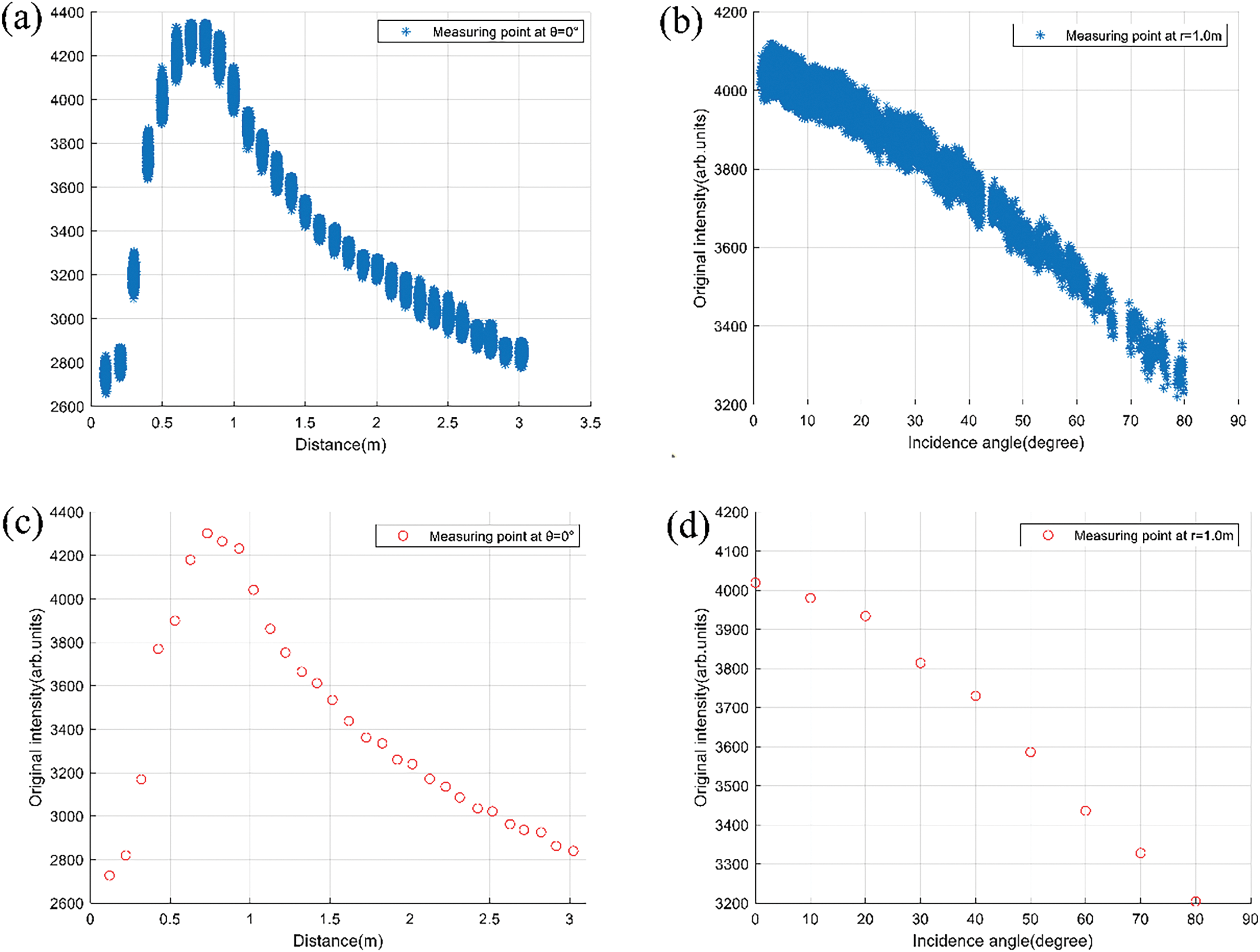
Figure 7: Distribution of modeling samples obtained by MLS and TLS modeling methods. (a) MLS modeling method distance and intensity modeling samples; (b) MLS modeling method incidence angle and intensity modeling sample; (c) TLS modeling method distance and intensity modeling samples; (d) TLS modeling method incidence angle and intensity modeling sample

By comparing Fig. 7a with Fig. 7c and Fig. 7b with Fig. 7d, it can be seen that the training data change trends of the MLS and TLS modeling methods are consistent, but the former has a significant advantage in the number of modeling data. More importantly, the distance, incidence angle, and intensity data of the MLS modeling method are derived from actual measurements rather than relying on statistical estimation. This unique data acquisition method enables the intensity correction model constructed based on the MLS modeling method to more accurately reveal the relationships between intensity and distance and between intensity and incidence angle, improving the reliability of the model.

3.2.2 Modeling Results

Table 2 shows the RMSE values of the distance piecewise polynomial and the incidence angle cosine polynomial calculated from the training data of the MLS and TLS modeling methods at different polynomial orders. Among them, KMLS, LMLS, and MMLS respectively represent the orders of the short-distance segment polynomial , the long-distance segment polynomial , and the incidence angle cosine polynomial in the MLS modeling method. Similarly, KTLS, LTLS, and MTLS represent the corresponding orders in the TLS modeling method.

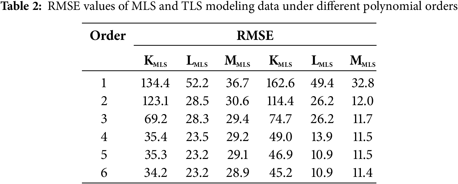
It can be seen from Table 2 that as the polynomial order value increases, the RMSE values of both modeling methods show a decreasing trend and tend to stabilize after a certain order value. According to the elbow rule, when the polynomial order values are set to K = 4, L = 4, and M = 2, the RMSE values of both modeling methods reach a stable state, indicating that the polynomial fitting effect is optimal. Based on this optimal fitting result, the specific expressions of and in the MLS and TLS modeling methods are determined, as shown in Table 3. By substituting and with specific parameters into Eq. (4) in Section 2.1.1, the final intensity correction model is established.

3.3 Results and Discussion

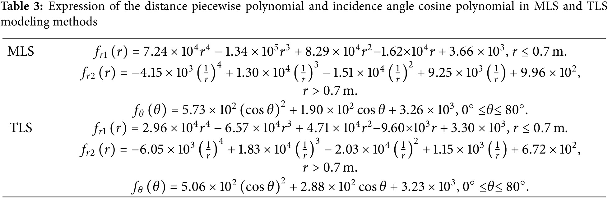
Table 4 shows the statistical analysis results of the intensity correction of the test set by the MLS and TLS modeling methods. In this table, for Test Set 1 and Test Set 2, the original intensity variation coefficient , the corrected intensity variation coefficient , and the ε value are listed, respectively.

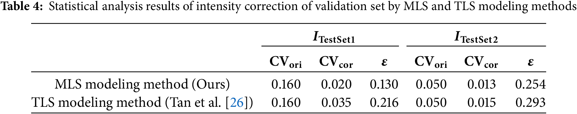
Based on the data in Table 4, it can be seen that in both test sets, the MLS modeling method is superior to the TLS modeling method in reducing the variability of the intensity data. For Test Set 1 with a large variation range of distance values, the correction effect of the MLS modeling method is significantly better than that of the TLS modeling method; for Test Set 2 with a large variation range of incidence angle values, the MLS modeling method still has an advantage but is relatively small, which may be attributed to the fact that the influence of the incidence angle on the intensity is not as significant as that of the distance.

For Test Set 1, the MLS modeling method reduces the original intensity variation coefficient from 0.160 to 0.020, and the calculated ε value is 0.130. This result indicates that the variability of the corrected intensity data is reduced to 0.130 times that of the original intensity, that is, the intensity consistency is improved to 7.692 times the original. In contrast, in the correction result of the TLS modeling method, is 0.035 and the ε value is 0.216, that is, the variability of the corrected intensity data is reduced to 0.216 times that of the original intensity, and the intensity consistency is improved to 4.630 times the original.

For Test Set 2, the MLS modeling method reduces from 0.050 to of 0.013, and the ε value is 0.254, meaning that the variability of the corrected intensity data is reduced to 0.254 times that of the original intensity, and the intensity consistency is improved to 3.937 times the original. In the TLS modeling method after correction, is 0.015 and the ε value is 0.293, that is, the variability of the corrected intensity data is reduced to 0.293 times that of the original intensity, that is, the intensity consistency is improved to 3.413 times the original.

Fig. 8a,b intuitively shows the distribution of the original intensity of the point cloud in the two test sets. It can be seen that the original intensity data shows a large fluctuation characteristic due to the changes in distance and incidence angle. In Test Set 1, the intensity value increases with the increase of distance at sites from 0.1 to 0.7 m and gradually decreases at sites from 0.7 to 3 m. In Test Set 2, the intensity value gradually decreases at sites with incidence angles from 0° to 80°.

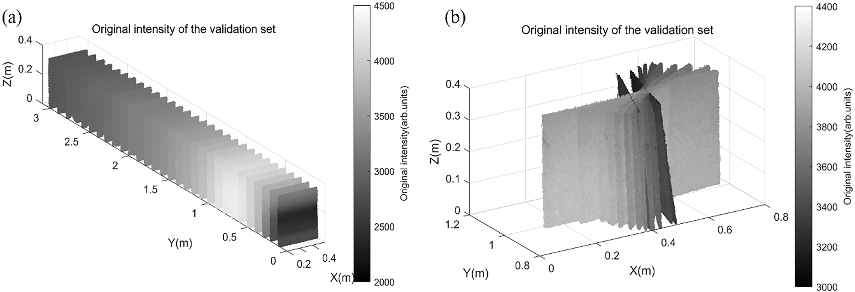
Figure 8: Original intensity distribution of verification point cloud obtained from distance and incidence angle experiment. (a) Original intensity distribution of verification point cloud obtained from distance experiment; (b) Original intensity distribution of verification point cloud obtained from incidence angle experiment

Fig. 9a–d shows the point cloud intensity distribution results after intensity correction of the test set by the MLS and TLS modeling methods.

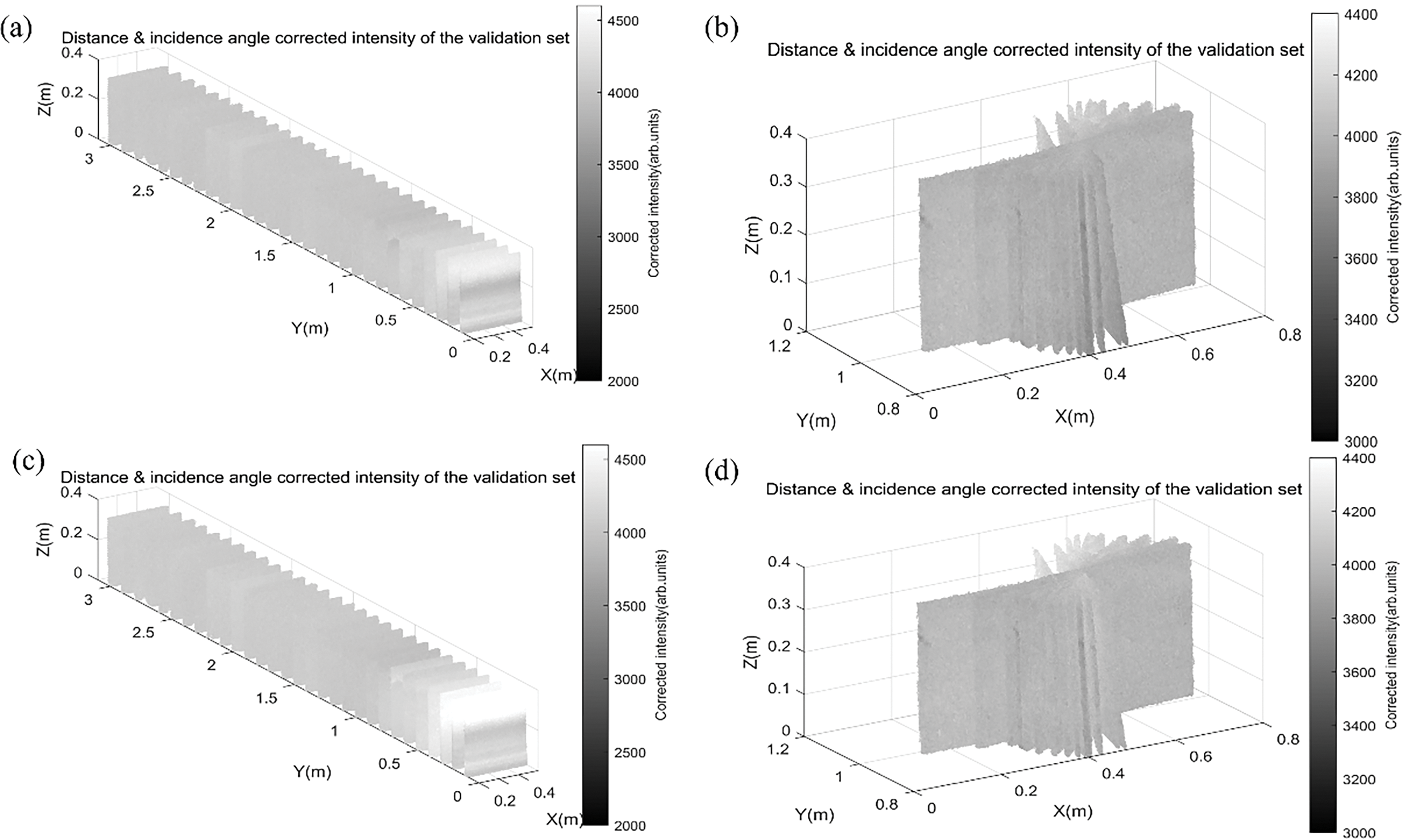
Figure 9: The point cloud intensity distribution results after intensity correction of the test set by the MLS and TLS modeling methods. (a) The intensity distribution of Test Set 1 after correction by the MLS modeling method; (b) The intensity distribution of Test Set 2 after correction by the MLS modeling method; (c) The intensity distribution of Test Set 1 after correction by the TLS modeling method; (d) The intensity distribution of Test Set 2 after correction by the TLS modeling method

By comparing Fig. 9a with Fig. 9c, for Test Set 1, the correction effect of the MLS modeling method is significantly better than that of the TLS modeling method, especially in the short-distance range of less than 0.7 m. However, in the distance range from 0.1 to 0.3 m, due to the combined influence of distance and incidence angle, the intensity data changes drastically, resulting in fitting errors in the intensity correction models of both modeling methods, and the correction effect is not good. This phenomenon is likely attributed to the inherent distance measurement errors and incidence angle calculation inaccuracies of the LiDAR system. According to existing research, the UTM-30LX-EW LiDAR employed in this study exhibits intensity fluctuation errors ranging from 200 to 300 even under constant distance and incidence angle conditions with specific reflectance targets. These fluctuations are further amplified when both distance and incidence angle values increase dramatically. Therefore, the observed anomalies primarily stem from the intrinsic high variability of the intensity data itself.

By comparing Fig. 9b with Fig. 9d, for Test Set 2, it can be observed that the correction effect of the MLS modeling method is also better than that of the TLS modeling method, especially in the intensity data with a large incidence angle range. However, in the edge area of the diffuse reflector plate at some sites with a large incidence angle range, the intensity correction effects of both the MLS and TLS modeling methods show slight defects. This phenomenon is presumably caused by the compounded effect of intensity fluctuation errors resulting from significant variations in both incidence angle and distance values near the edge regions, thereby increasing the fitting errors of the correction models.

In conclusion, the intensity correction anomalies observed in both Test Sets 1 and 2 highlight the limitations of current models in handling high-intensity fluctuations and complex conditions. Future research should focus on developing more sophisticated models to better characterize and correct intensity data, thereby enhancing the accuracy and robustness of LiDAR intensity correction.

4  Conclusions

1.    This study proposes a fine-grained point cloud intensity correction modeling method based on MLS technology to address the problem of limited model accuracy in the traditional TLS intensity correction modeling method.

2.    In the implementation of the method, first, the MLS technology is used to continuously scan the standard diffuse reflector plate with a reflectivity of 50% to collect point cloud data at different distances and incidence angles. Then, a fine-grained screening strategy is adopted to accurately screen out the training data that can reflect the single-variable relationships between intensity and distance and between intensity and incidence angle from the collected point cloud. Finally, based on these training data, a high-precision intensity correction model suitable for the UTM-30-LX-EW 2D LiDAR is successfully constructed through a polynomial fitting function.

3.    To verify the effectiveness of the proposed method, the root mean square error RMSE, the coefficient of variation CV, and the variance-to-mean ratio are used as evaluation metrics to compare the MLS modeling method with the traditional TLS modeling method on the same test set. The experimental results show that in Test Set 1 with a large variation range of distance values, the intensity consistency after correction by the MLS modeling method is significantly improved, reaching 7.692 times that of the original intensity, while the TLS modeling method only improves to 4.630 times that of the original intensity. In Test Set 2 with a large variation range of incidence angle values, although the advantage of the MLS modeling method is relatively small, it still improves the intensity consistency to 3.937 times that of the original intensity, slightly better than 3.413 times that of the TLS modeling method. These experimental results fully prove that the method proposed in this study has a significant effect in improving the accuracy of intensity correction modeling.

Future research will focus on fine-grained screening of training data to explore advanced modeling techniques, such as the lookup table method, aiming to further enhance the accuracy and practicality of intensity correction modeling.

Acknowledgement: This research is supported in part by the National Natural Science Foundation of China under grant number 31901239.

Funding Statement: This work is funded by Researchers Supporting Project Number (RSPD2025R947), King Saud University, Riyadh, Saudi Arabia.

Author Contributions: The authors confirm contribution to the paper as follows: study conception and design: Xu Liu, Qiujie Li, Youlin Xu, Fa Zhu; data collection: Xu Liu, Qiujie Li, Musaed Alhussein, Khursheed Aurangzeb; analysis and interpretation of results: Xu Liu, Qiujie Li, Youlin Xu, Fa Zhu; draft manuscript preparation: Xu Liu, Qiujie Li, Musaed Alhussein, Khursheed Aurangzeb. All authors reviewed the results and approved the final version of the manuscript.

Availability of Data and Materials: Not applicable.

Ethics Approval: Not applicable.

Conflicts of Interest: The authors declare no conflicts of interest to report regarding the present study.

References

1. Mercier A, Myllymäki M, Hovi A. Exploring the potential of SAR and terrestrial and airborne LiDAR in predicting forest floor spectral properties in temperate and boreal forests. Remote Sens Environ. 2025;316(22):114486–96. doi:10.1016/j.rse.2024.114486. [Google Scholar] [CrossRef]

2. Yang Y, Yuan G. High precision DSRC and LiDAR data integration positioning method for autonomous vehicles based on CNN. Comput Electr Eng. 2024;120:109741–52. doi:10.1016/j.compeleceng.2024.109741. [Google Scholar] [CrossRef]

3. Xiao Y, Liu Y, Luan K. Deep LiDAR-radar-visual fusion for object detection in Urban environments. Remote Sens. 2023;15(18):4433–45. doi:10.3390/rs15184433. [Google Scholar] [CrossRef]

4. Yun T, Eichhorn MP, Jin S. A framework for phenotyping rubber trees under intense wind stress using laser scanning and digital twin technology. Agr For Meteorol. 2025;361(2):110319–31. doi:10.1016/j.agrformet.2024.110319. [Google Scholar] [CrossRef]

5. Yun T, Li J, Status ML. Advancements and prospects of deep learning methods applied in forest studies. Int J Appl Earth Obs. 2024;131(8):103938–46. doi:10.1016/j.jag.2024.103938. [Google Scholar] [CrossRef]

6. Luo R, Zhou ZX, Xi C. 3D deformation monitoring method for temporary structures based on multi-thread LiDAR point cloud. Measurement. 2022;200(3):10112–24. doi:10.1016/j.measurement.2022.111545. [Google Scholar] [CrossRef]

7. Jiang J, Liu F, Liu Y. A dynamic ensemble algorithm for anomaly detection in IoT imbalanced data streams. Comput Commun. 2022;194(5):250–7. doi:10.1016/j.comcom.2022.07.034. [Google Scholar] [CrossRef]

8. Jiang J, Liu F, Ng WY. Dynamic incremental ensemble fuzzy classifier for data streams in green internet of things. IEEE T Green Commun Netw. 2022;6(3):1316–29. doi:10.1109/TGCN.2022.3151716. [Google Scholar] [CrossRef]

9. Paulina S, Czesław S, Miłosława R. Crack detection in building walls based on geometric and radiometric point cloud information. Automat Constr. 2022;134(5):1023–35. doi:10.1016/J.AUTCON.2021.104065. [Google Scholar] [CrossRef]

10. Junttila S, Hölttä T, Puttonen E. Terrestrial laser scanning intensity captures diurnal variation in leaf water potential. Remote Sens Environ. 2021;255(02):1125–37. doi:10.1016/j.rse.2020.112274. [Google Scholar] [CrossRef]

11. Junttila S, Holopainen M, Vastaranta M. The potential of dual-wavelength terrestrial lidar in early detection of Ips typographus (L.) infestation—leaf water content as a proxy. Remote Sens Environ. 2019;231(3):111264. doi:10.1016/j.rse.2019.111264. [Google Scholar] [CrossRef]

12. Wang L, Chen H, You Z. Combining geometrical and intensity information to recognize vehicles from super-high density UAV-LiDAR point clouds. Sci Rep. 2024;14(1):25097–605. doi:10.1038/s41598-024-75968-z. [Google Scholar] [PubMed] [CrossRef]

13. Naich AY, Carrión JR. LiDAR-based intensity-aware outdoor 3D object detection. Sensors. 2024;24(9):2942–54. doi:10.1038/S41598-024-75968-Z. [Google Scholar] [CrossRef]

14. Bai J, Niu Z, Wang L. A theoretical demonstration on the independence of distance and incidence angle effects for small-footprint hyperspectral LiDAR: basic physical concepts. Remote Sens Environ. 2024;315(9):114452–62. doi:10.1016/J.RSE.2024.114452. [Google Scholar] [CrossRef]

15. Qi B, Yang G, Zhang Y. Target intensity correction method based on incidence angle and distance for a pulsed Lidar system. Appl Optics. 2024;63(10):86–97. doi:10.1364/AO.505690. [Google Scholar] [PubMed] [CrossRef]

16. Sun JF, Zhou X, Fan ZG. Investigation of light scattering properties based on the modified Li-Liang BRDF model. Infrared Phys Tech. 2021;78(8):1125–37. doi:10.1016/J.INFRARED.2021.103992. [Google Scholar] [CrossRef]

17. Tian WX, Tang LL, Chen YW. Analysis and radiometric calibration for backscatter intensity of hyperspectral LiDAR caused by incidence angle effect. Sensors. 2021;21(9):1203–16. doi:10.3390/S21092960. [Google Scholar] [PubMed] [CrossRef]

18. Carrea D. Correction of terrestrial LiDAR intensity channel using Oren-Nayar reflectance model: an application to lithological differentiation. ISPRS J Photogramm. 2016;15(3):1112–26. doi:10.1016/j.isprsjprs.2015.12.004. [Google Scholar] [CrossRef]

19. Maru MB, Wang Y, Kim H, Yoon H, Park S. Improved building facade segmentation through digital twin-enabled RandLA-Net with empirical intensity correction model. J Build Eng. 2023;78(6):1129–45. doi:10.1016/J.JOBE.2023.107520. [Google Scholar] [CrossRef]

20. Höfle B, Pfeifer N. Correction of laser scanning intensity data: data and model-driven approaches. ISPRS J Photogramm Remote Sens. 2007;62(6):415–33. doi:10.1016/j.isprsjprs.2007.05.008. [Google Scholar] [CrossRef]

21. Li XL, Shang YH, Hua BC. LiDAR intensity correction for road marking detection. Opt Laser Eng. 2023;160(2):1456–69. doi:10.1016/j.optlaseng.2022.107240. [Google Scholar] [CrossRef]

22. Liu Z, Wang T, Zhu F. Domain adaptive learning based on equilibrium distribution and dynamic subspace approximation. Expert Syst Appl. 2024;249(2):123673–84. doi:10.1016/j.eswa.2024.123673. [Google Scholar] [CrossRef]

23. Liu Z, Zhu F, Xiong H. Graph regularized discriminative nonnegative matrix factorization. Eng Appl Artif Intel. 2025;139(2):109629–36. doi:10.1016/j.engappai.2024.109629. [Google Scholar] [CrossRef]

24. Zhu F, Gao J, Yang J. Neighborhood linear discriminant analysis. Pattern Recognit. 2022;123(6):108422–35. doi:10.1016/j.patcog.2021.108422. [Google Scholar] [CrossRef]

25. Saranti A, Pfeifer B, Gollob C. From 3D point-cloud data to explainable geometric deep learning: state-of-the-art and future challenges. Wires Data Min Knowl. 2024;14(6):1554–9. doi:10.1002/widm.1554. [Google Scholar] [CrossRef]

26. Tan K, Cheng XJ. Distance effect correction on TLS intensity data using naturally homogeneous targets. IEEE Geosci Remote Sens Lett. 2020;17(3):499–503. doi:10.1109/LGRS.2019.2922226. [Google Scholar] [CrossRef]

27. Nathan S, Estelle B, Mustapha ME. Radiometric correction of laser scanning intensity data applied for terrestrial laser scanning. ISPRS J Photogramm. 2021;172(2):1–16. doi:10.1016/j.isprsjprs.2020.11.015. [Google Scholar] [CrossRef]

28. Xu T, Xu L, Yang B. Terrestrial laser scanning intensity correction by piecewise fitting and overlap-driven adjustment. Remote Sens. 2017;9(11):1090–100. doi:10.3390/rs9111090. [Google Scholar] [CrossRef]

29. Tan K, Cheng XJ. Correction of incidence angle and distance effects on TLS intensity data based on reference targets. Remote Sens. 2016;8(3):251–63. doi:10.3390/rs8030251. [Google Scholar] [CrossRef]

30. Bolkas D. Terrestrial laser scanner intensity correction for the incidence angle effect on surfaces with different colors and sheens. INT J Remote Sens. 2019;40(18):7169–89. doi:10.1080/01431161.2019.1601283. [Google Scholar] [CrossRef]

31. Zhao Z, Gan S, Xiao B. Three-dimensional reconstruction of Zebra crossings in vehicle-mounted LiDAR point clouds. Remote Sens. 2024;16(19):3722–34. doi:10.3390/rs16193722. [Google Scholar] [CrossRef]

32. Shokri D, Zaboli M, Dolati F. POINTNET++ transfer learning for tree extraction from mobile LIDAR point clouds. ISPRS Ann Photogramm Remote Sens Spatial Inf Sci. 2023;X-4/W1-2022:721–7. doi:10.5194/ISPRS-ANNALS-X-4-W1-2022-721-2023. [Google Scholar] [CrossRef]

33. Benedetto A, Fiani M. Distress detection in tunnel lining from MLS data. Procedia Struct Integr. 2024;64(3):2254–62. doi:10.1016/j.prostr.2024.09.355. [Google Scholar] [CrossRef]

34. Chutian G, Guo M, Zheng J. An automated multi-constraint joint registration method for mobile LiDAR point cloud in repeated areas. Measurement. 2023;222(5):1245–58. doi:10.1016/J.MEASUREMENT.2023.113620. [Google Scholar] [CrossRef]

35. Li QJ, Xue YX. Total leaf area estimation based on the total grid area measured using mobile laser scanning. Comput Electron Agric. 2023;204(5):1356–69. doi:10.1016/j.compag.2022.107503. [Google Scholar] [CrossRef]

36. Chabert JL, Peruginelli G. Adelic versions of the Weierstrass approximation theorem. J Pure Appl Algebra. 2018;222(3):568–84. doi:10.1016/j.jpaa.2017.04.020. [Google Scholar] [CrossRef]

37. Adcock B, Huybrechs D, Piret C. Stable and accurate least squares radial basis function approximations on bounded domains. SIAM J Numer Anal. 2024;62(6):2698–718. doi:10.1137/23M1593243. [Google Scholar] [CrossRef]