XGBoost-Liver: An Intelligent Integrated Features Approach for Classifying Liver Diseases Using Ensemble XGBoost Training Model

1  Introduction

The liver is a complex and multifunctional organ, playing a pivotal role in digestion, metabolism, detoxification, and immune defense, making it indispensable for overall health. Despite its remarkable regenerative capabilities and adaptability, the liver remains highly vulnerable to infections, injuries, and genetic disorders that can compromise its functions and pose serious health risks. Such conditions can lead to chronic inflammation, jaundice, and other complications, significantly impacting quality of life and longevity. Addressing these challenges requires a deeper understanding of the factors contributing to liver dysfunction and the development of effective diagnostic and preventative strategies. Early detection and timely interventions are crucial for managing liver diseases (LD), reducing associated mortality, and improving patient outcomes. The healthcare industry has undergone substantial transformations in its delivery systems and organizational structures due to advancements in data processing, primarily through ML (Machine Learning) and Artificial Intelligence (AI). These innovations have revolutionized how data is collected, stored, and analyzed, enabling clinical practitioners to incorporate advanced decision-making models into traditional healthcare practices. This integration has significantly enhanced diagnostic accuracy and informed decision-making across the sector. Notably, the progressive development of AI and ML applications has made early illness prediction feasible for conditions such as diabetes, hypertension, COPD, and cardiovascular diseases. By leveraging big data, these technologies provide critical insights into diagnosis, prognosis management, and treatment, complementing preventative measures that promote healthy behavior. The ongoing integration of AI and ML into healthcare is paving the way for advancements in precision medicine, drug discovery, and diagnostic tools, with implications for improved healthcare delivery, personalized treatment, and overall population health outcomes.

Numerous ML techniques have been explored for the classification of liver disease. In 2016, Prasad Babu et al. [1] introduced a K-means clustering methodology for liver illness detection, utilizing various classification models to evaluate its effectiveness. Their results revealed accuracies of 56% for Naive Bayes (NB), 64% for K-Nearest Neighbors (KNN), and 69% for the C4.5 decision tree classifier. Similarly, Gan et al. [2] examined multiple classification methods for liver disease prediction and demonstrated that their AdaC-TANBN approach, combining AdaBoost with a modified Tree-Augmented Naive Bayes (TANBN) model, achieved an accuracy of 69.03%. Anagaw et al. [3] proposed an advanced classification model employing Complement Naive Bayes (CNB), gaining 71.36% accuracy, outperforming traditional Naive Bayes classifiers. Further advancements include Sreejith et al. [4], who applied Chaotic Multi-Verse Optimization (CMVO) for feature selection alongside the Synthetic Minority Over-sampling Technique (SMOTE), achieving 82.62% accuracy on the ILPD dataset. Kumar et al. introduced a Variable-NWFKNN approach to enhance liver disease classification accuracy, attaining 87.71% using 10-fold cross-validation and addressing dataset imbalance with Tomek connections and redundancy-based under-sampling (TR-RUS). Kuzhippallil et al. [5] improved classification accuracy to 88% by employing advanced data preparation and feature selection methods. Most recently, Amin et al. [6] presented a sophisticated projection-based statistical feature selection and classification technique using the ILPD dataset, achieving 88.10% accuracy with Support Vector Machine, Logistic Regression, and Random Forest methods. These developments underscore the evolving role of machine learning in enhancing the accuracy and efficiency of liver disease diagnosis, enabling timely and effective medical interventions.

This study proposes a comprehensive and novel approach to predicting liver disease. A random oversampling strategy is applied to address the challenges of overfitting and class imbalance during model development. Next, we employ two distinct feature selection methodologies: Ranking-based strategies, including Analysis of Variance (ANOVA) and Chi-Square (CHI2), and Statistical Projection-based strategies, comprising Principal Component Analysis (PCA) and Linear Discriminant Analysis (LDA). These methods rank and evaluate each feature’s relevance to the target class of liver illness. Subsequently, a hybrid feature vector is constructed by combining all four feature sets. The Fisher score method is employed for feature selection to enhance computational efficiency and identify the most impactful features. The proposed model is called XGBoost-Liver, and its framework is shown in Fig. 1. Diverse machine learning models, including Logistic Regression (LR), K-Nearest Neighbor (KNN), Random Forest (RF), Support Vector Machine (SVM), and Naive Bayes (NB), are leveraged to evaluate prediction performance. The proposed methodology undergoes rigorous performance assessment using metrics such as the Matthews Correlation Coefficient, Accuracy, Sensitivity, Specificity, and Area Under the Curve (AUC). The results demonstrate the superior predictive capability of the XGBoost (EXtreme Gradient Boosting) model, providing valuable insights for early liver disease detection, improving diagnostic precision, and facilitating timely medical interventions.

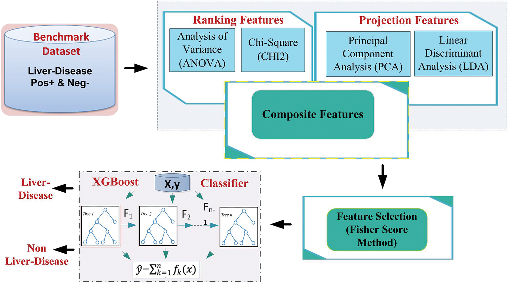
Figure 1: The architecture of the proposed XGBoost-liver

2  Proposed Model Framework

2.1 Benchmark Dataset

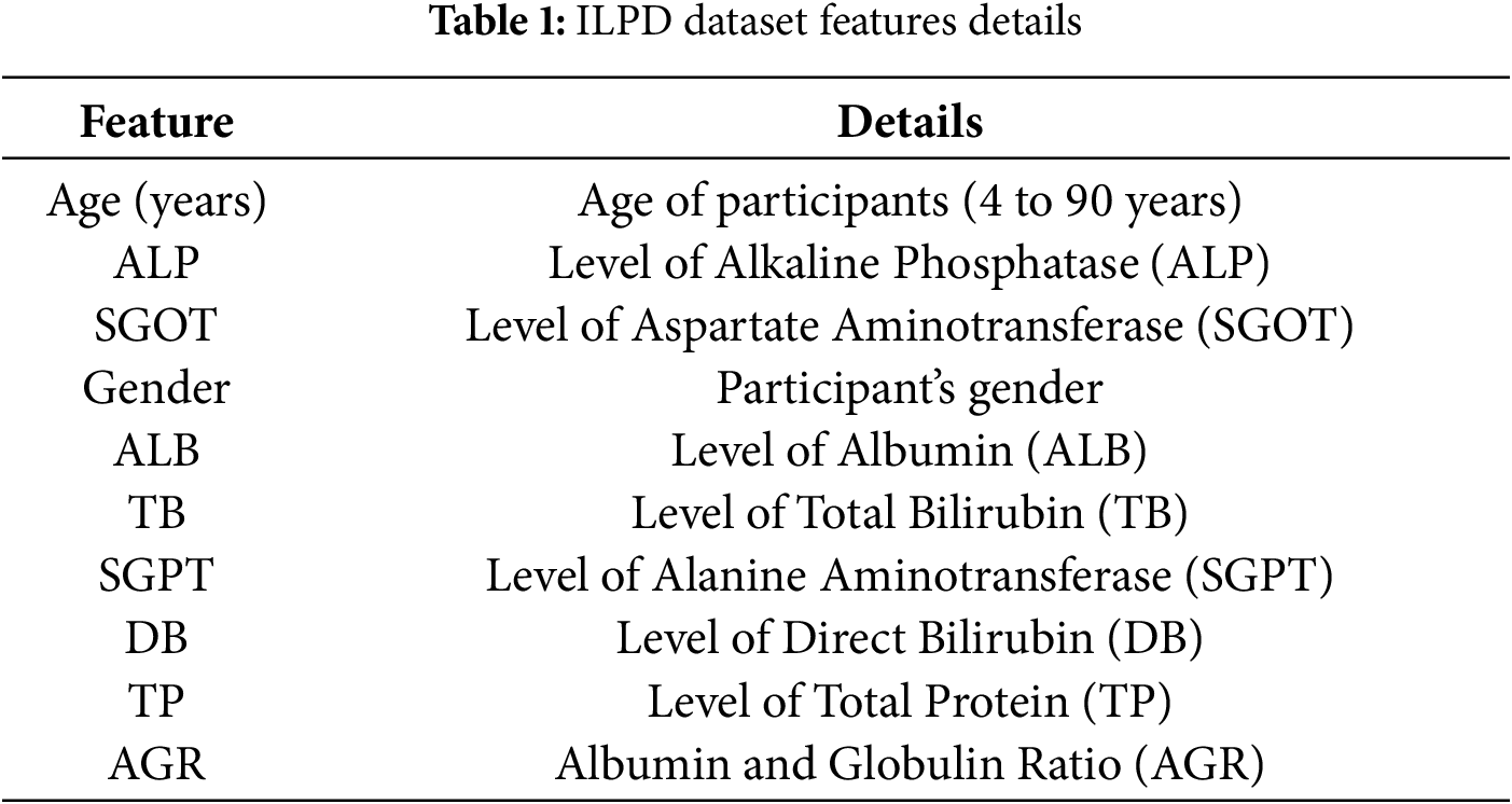
According to Chou’s review, using a reliable and valid dataset is essential for building robust and powerful computational models. Our study used the Indian Liver Patient Dataset (ILPD) [6], a well-known benchmark dataset. The ILPD contains 583 records with ten different features. Table 1 summarizes the dataset, which includes 439 male participants (75.30%) and 144 female participants (24.70%). The main focus of the dataset is to help diagnose liver disease by identifying whether participants have the condition. The long-term liver disease risk is addressed as a classification challenge with “Liver-Disease” (LD) or “Non-Liver-Disease” (Non-LD) classes. The total dataset comprises 416 positive cases of liver disease and 167 controlled cases. Considering the significance of balanced datasets in machine learning analysis, we applied a data balancing technique, i.e., Random oversampling, resulting in a dataset of 832 cases, evenly distributed between instances of liver disease and non-disease cases (i.e., LD = 416, Non-LD = 416).

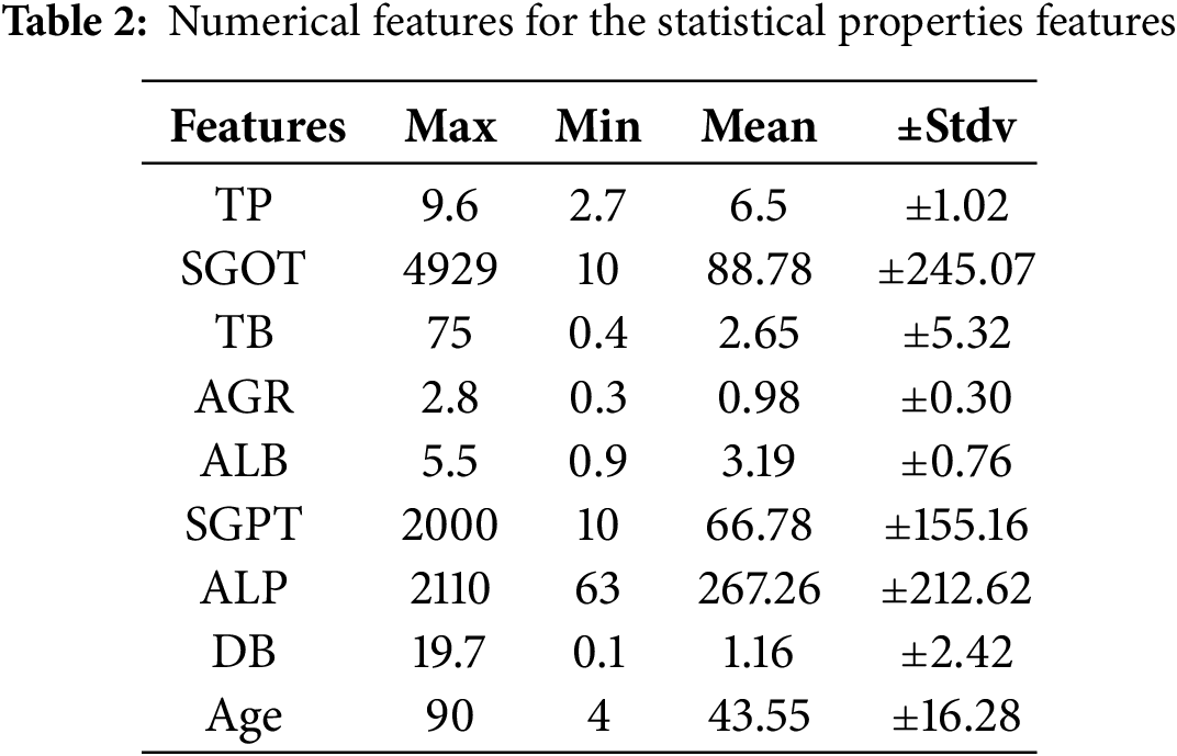
Statistical aspects of the features in the balanced dataset are shown in Table 2, with key values such as standard deviation, mean, minimum, and maximum for each variable. The numerical distributions of the dataset are thoroughly examined in this investigation. Table 2 provides numerical distribution analysis by summarising the statistical attributes of features, such as max, min, mean, and standard deviation.

2.2 Feature Formulation Technique

ML algorithms often face the obscenity of dimensionality, which arises when there are many data points but relatively few meaningful features or when the feature space contains irrelevant information [7]. To address this challenge, we first implement two ranking methods [8], i.e., Analysis of Variance (ANOVA) and Chi-Square (CHI2), to examine the involvement of each feature to the target class (i.e., liver disease). Subsequently, we used a statistical projection-based strategy comprising PCA and LDA, which rely on statistics to identify essential features. To select the most impactful features, we used the Fisher Score method as a feature selection. The Fisher score method helps to simplify the dataset by making it easier to analyze and reducing the computing power needed [9,10].

2.2.1 CHI-SQUARE (CHI2)

CHI2 is a widely used filter feature selection method, and it is called Chi-Square (Chi2). It’s a handy tool that relies on statistical information. Chi2 helps us understand whether there’s a connection between two or unrelated variables. It’s like a test we use in statistics to examine two separate observations. In text classification, these separate observations are the words we use and the categories they belong to. To calculate Chi2 information:

(1)

The variables N and E denote the memorialized and expected frequencies for each case of term t and class C. The mathematical form of the Chi2 method used in this study is given in Eq. (2).

(2)

2.2.2 Analysis of Variance (ANOVA)

The ANOVA F-Score is a statistical method used to rank features based on their ability to distinguish between classes by analyzing the variance within and between groups. It measures how much the mean value of a feature varies across different classes compared to the variability within each class. Features with higher F-scores are more effective at separating classes, making them valuable for classification tasks. This method is computationally efficient, easy to implement, and works well for datasets with continuous features and categorical targets, making it a popular choice for feature selection in machine learning workflows. For a feature f and a dataset with c classes, the F-Score is defined as:

(3)

where c represents the number of classes, Nj is the number of samples in class j . μj represents the mean value of feature f for class j, μ represents the overall mean value of feature f, N is the total number of samples, jk is the value of feature f for the k-th sample in class j, and Cj is the set of samples in class j.

2.2.3 Linear Discriminant Analysis (LDA)

Linear Discriminant Analysis (LDA) is a supervised dimensionality reduction technique that projects data onto a lower-dimensional space while maximizing class separability. The main goal of LDA is to find a transformation matrix W that maximizes the ratio of between-class variance to within-class variance, ensuring that different classes are well-separated in the projected space. Mathematically, the objective function of LDA is to maximize the following criterion. Where Sb is the between-class scatter matrix, Sw is the within-class scatter matrix, and W is the transformation matrix to be optimized.

(4)

2.2.4 Principle Components Analysis (PCA)

PCA reduces data dimensions using covariance matrices [11] with minimum loss of discriminative features. Let’s consider a feature vector S with the dimension of i * j, where “i” represents the number of extracted features and “j” represents the number of samples. Let “k” represent the number of desired features. The value of “k” must be less than “i”. Let’s consider the following input feature vector S using Eq. (5):

(5)

Through the PCA algorithm, we implemented the following steps to reduce the dimensionality of the feature vector:

Step 1: Compute the mean

(6)

Step 2: Subtract the mean

(7)

Step 3: Compute the covariance

(8)

where and T = transpose of a matrix.

Step 4: Calculate the eigenvalues in ascending order. The first eigenvalue should be greater than the second and fourth.

(9)

Step 5: Compute the corresponding eigenvectors

(10)

Last step: Select k eigenvectors corresponding to the largest eigenvalues to reconstruct a new set of feature vectors in the space. This selection process helps avoid dimensionality problems, keeping the most essential data. It also improves the computational speed and interpretability of various other tasks being performed in the analytical methods of the dataset, which is the main aim of PCA in the case of data preprocessing and data analysis.

(11)

2.3 Hybrid Feature

The methodology proposed in this paper incorporates four feature extraction mechanisms, detailed in Section 2.2. These mechanisms are combined to construct a hybrid feature vector, as defined in Eq. (12). Mathematically referred to as the hybrid feature vector, it integrates features contributed by each technique (10 dimensions per method) to form a unified representation comprising 40 dimensions.

(12)

2.4 Feature Selection Methods

An essential step in machine learning and statistics is feature selection, which means picking out relevant features to build a forecast model. Feature selection lessens the “curse of dimensionality” by making the dataset less multidimensional. This speeds up training times and can sometimes improve model performance. Much research has shown that choosing the right features for data can make it work better with some learning models and help store naturally occurring patterns in the input space [12,13]. There are two main types of feature selection methods: supervised and unsupervised. Labeled datasets are treated with supervised methods that look for features that make supervised learning models work better, like those used in classification and regression tasks. Unsupervised methods are used to find natural trends for unlabeled data without setting goal labels ahead of time.

This study employs XGBoost, a supervised learning method, and therefore relies on supervised feature selection techniques. Specifically, this work proposes the filter method for feature selection, leveraging its ability to evaluate and rank features based on statistical criteria independently of the learning algorithm. This approach ensures the selection of the most relevant features, optimizing model performance. In filter methods, the chosen features don’t depend on the algorithm being used. They use the general features of the training data to select features that aren’t related to any prediction. Instead of the error rate, filter methods always use a reference measure to rank the scores of features. In this study, we used the filter method (i.e., the Fisher score method), which finds the lengths between each feature’s data points. Fig. 2 shows the top 10 features using SHAP to visualize the impact of these selected features. In the Fisher score method, feature scores are ranked by this rule: a feature gets a better score if the distances between data points in different classes are longer but not if the distances between data points in the same class are shorter. The Fisher score method is shown below:

(13)

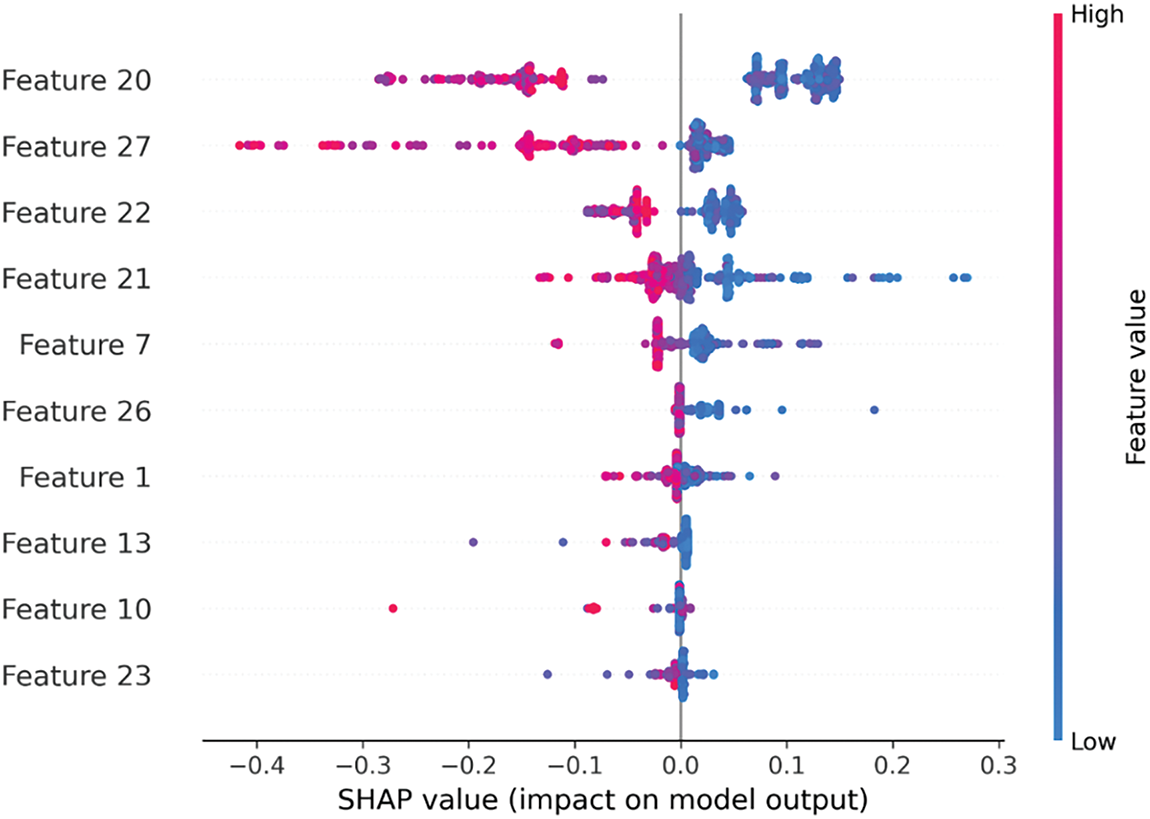
Figure 2: Vital features selected from hybrid features using the Fisher score method

The variables represent the average of the a-th feature across the entire dataset and within the positive and negative subsets, respectively. Here, j corresponds to the j-th sample of the a-th feature. The numerator quantifies the distinction between the positive and negative subsets, while the denominator measures the variation within each subset. A higher Fisher score indicates that the feature is more discriminative.

2.5 XGBoost

XGBoost is a gradient-boosting library that delivers faster, more flexible, and scalable machine learning. It employs gradient boosting, an ensemble learning algorithm that combines the outputs of multiple weak learners, typically decision trees, to build a robust predictive model. A specialized matrix class in XGBoost improves data storage and access efficiency, enhancing performance during training and evaluation. XGBoost minimizes the mean squared error (MSE) between actual and predicted values for regression tasks. It supports various loss functions, such as squared error, absolute error, and Huber loss, to guide Optimization. The objective function assesses overall model performance, while the loss function evaluates the difference between predicted and actual values, as illustrated in Fig. 3.

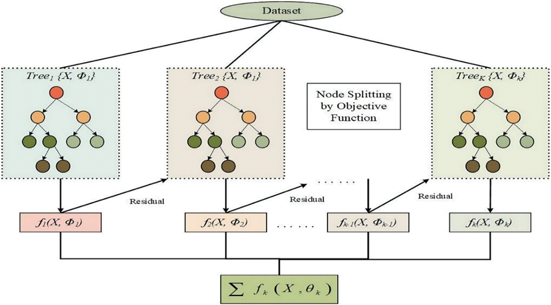
Figure 3: The workflow of the XGBoost algorithm

XGBoost trains models in stages by sequentially adding new trees to correct errors made by the previous ones, guided by the negative gradient of the loss function. Cross-validation is a crucial technique for evaluating XGBoost’s performance, where the dataset is divided into subsets to enable multiple rounds of training and validation. The XGBoost classifier supports binary and multiclass classification objectives, such as logistic regression and Softmax. Seamlessly integrating with scikit-learn, XGBoost allows users to switch between its native API and scikit-learn’s API without compatibility issues, facilitating using other machine learning libraries to optimize model parameters.

3  Performance Evaluation

The efficiency of a machine learning system is quantified using various standard assessment metrics. For this study, we employed commonly used performance measures, including Accuracy (ACC), Specificity (SP), Sensitivity (SN), the Area Under the Receiver Operating Characteristic Curve (AUC), and the Matthews Correlation Coefficient (MCC). Accuracy (ACC) represents the overall correctness of the model’s predictions. Sensitivity (SN) measures the proportion of true positives identified correctly, while Specificity (SP) evaluates the proportion of true negatives. Sensitivity and Specificity are inversely related, as adjustments in the decision threshold can increase one metric at the expense of the other. Lowering the threshold increases Sensitivity but decreases Specificity, whereas raising it has the opposite effect [14]. The Matthews Correlation Coefficient (MCC) provides a balanced evaluation, accurately reflecting the model’s ability to identify positive and negative outcomes. Unlike other metrics, MCC is robust even in class imbalance, making it particularly useful for this study. The AUC score, derived from the Receiver Operating Characteristic (ROC) curve, plots the True Positive Rate (TPR, equivalent to Sensitivity) against the False Positive Rate (FPR, where FPR = 1 − Specificity). AUC is a threshold-independent metric, making it a reliable criterion for evaluating the model’s discrimination capability. These metrics using the Chou symbol are defined as:

(14)

(15)

(16)

(17)

where T+ symbolizes true positives, F+ symbolizes false positives, T− Symbolizes true negatives, and F− false negatives, respectively.

4  Results and Analysis

4.1 Experimental Setup

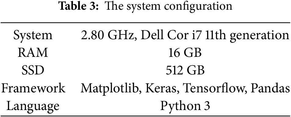
The experiments were conducted on a computing system configured with an 11th-generation Intel Core i7-1165G7 processor operating at 2.80 GHz, RAM of 16 GB, and a 512-GB SSD, running Windows 11 Home on a 64-bit architecture. This setup provided adequate computational power for data preprocessing, model training, and evaluation tasks. Including an SSD (Solid State Disk) ensured faster data access and improved system responsiveness compared to traditional HDDs (Hard Disk Drive). While this configuration was sufficient for handling moderate datasets and typical machine learning workflows, larger-scale datasets or resource-intensive tasks may necessitate further enhancements to the CPU (Central Processing Unit) and RAM (Random Access Memory). The software environment consisted of Python 3 and several essential data science and machine learning libraries. NumPy and SciPy were used for numerical computations, Matplotlib was used for data visualization, and Pandas was used for data preprocessing and analysis. TensorFlow and Keras were employed to design and evaluate DL (Deep Learning) models. This comprehensive suite of tools facilitated the efficient implementation, training, and testing of ML models. Standard metrics assessed the proposed model performance to measure prediction correctness, stability, and reliability. These metrics provided a detailed understanding of the model’s strengths and limitations, guiding further Optimization. The integration of this hardware-software combination enabled a seamless workflow for data processing and model validation, and the overall configuration of the system is presented in Table 3.

4.2 Hyper-Parameters Optimization

This section optimizes the suggested XGBoost model by using various hyper-parameter settings. XGBoost is a robust and highly customizable gradient-boosting library widely recognized for its ability to address complex machine-learning tasks. Its performance is primarily influenced by the careful tuning of hyper-parameters, which directly impact the model’s learning process, complexity, and ability to balance bias and variance. Table 4 outlines the primary hyper-parameters utilized in this study, i.e., the number of estimators, maximum tree depth, and the learning rate, along with a concise description of their roles and permissible value ranges. A grid search method optimized the parameters, systematically exploring all combinations of hyper-parameter values within defined intervals. Each configuration was evaluated on the training dataset, and the hyper-parameters minimizing the objective function error were selected to enhance model performance and mitigate over-fitting [10,15–17].

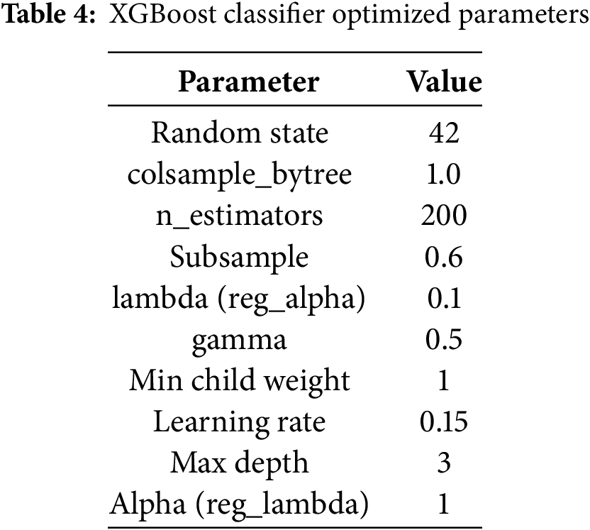
Moreover, the optimized hyper-parameters identified for our proposed XGBoost classifier include the maximum tree depth (i.e., 3) and the number of estimators (i.e., 200), ensuring deep learning capabilities. Regularization parameters like lambda and alpha, explored at 0.1 and 1, help prevent over-fitting by controlling complexity. The learning rate, a critical parameter for adjusting model updates, is set at 0.01 for gradual learning. Other parameters, such as the column sampling ratio and minimum child weight, are fine-tuned to enhance generalization. These parameters optimize model accuracy and performance, leveraging XGBoost’s powerful gradient-boosting capabilities.

Furthermore, the optimal hyper-parameters were also determined by selecting the combination that yielded the smallest Root Mean Squared Error (RMSE) across all tested configurations. Fig. 4 illustrates the variation in RMSE for each hyper-parameter across its search range, clearly highlighting the values associated with minimal RMSE. The optimal settings are identified based on these results: colsample_bytree set to 1, learning_rate to 0.15, max_depth to 3, and subsample to 0.6. These values, detailed in Table 4, ensure the best model performance by effectively balancing complexity and accuracy.

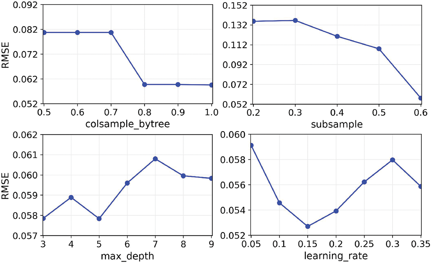
Figure 4: Relationship between RMSE and four major hyper-parameters

4.3 Performance Evaluation

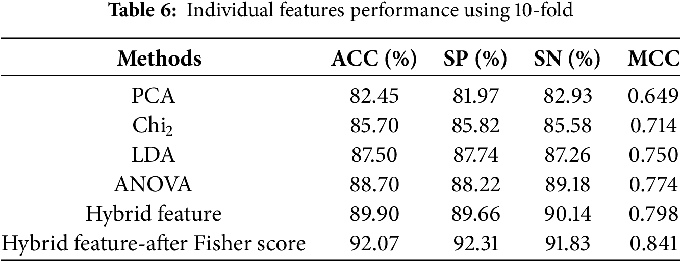
This section evaluates the XGBoost model’s prediction results using individual and hybrid feature methods. The XGBoost model’s efficacy was further enhanced using the Fisher feature selection method. In literature [18,19], researchers have used machine learning methods like k-fold cross-validation (CV) to assess model performance predictions. The results of the XGBoost method are verified in this paper by implementing a 5-fold and 10-fold cross-validation. Tables 5 and 6 illustrate the estimated outcomes that the proposed model achieved on the balanced dataset by employing a variety of feature vectors.

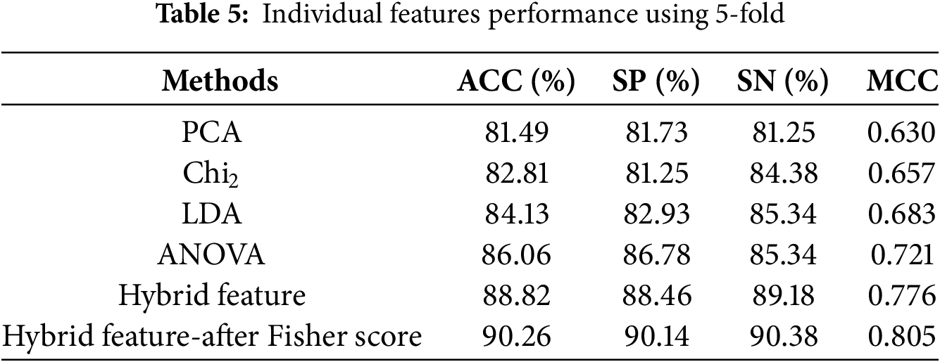
From Table 5, the proposed model outperformed using a hybrid features vector compared to the individual features by 5-fold cross-validation. The proposed model achieved an accuracy rate of 88.82% and an MCC of 0.776 utilizing a hybrid feature vector. In order to further enhance the performance of the proposed model, we apply the feature selection method, i.e., the Fisher score method. The selected features attained an accuracy of 90.26% and a MCC of 0.805.

Moreover, Table 6 demonstrates that the proposed model using 10-fold cross-validation attained superior performance with an optimized hybrid feature vector compared to the optimized hybrid features using 5-fold cross-validation. The proposed model achieved an accuracy rate of 92.07%, Sensitivity of 91.83%, Specificity of 92.31%, and an MCC of 0.841 utilizing an optimized hybrid feature vector. The experimental results demonstrate that the proposed model performs better using a resourceful feature set and applying 10-fold cross-validation to improve prediction accuracy and target result identification.

Additionally, a confusion matrix is presented in Fig. 5 to further explore the behavior of the proposed model in prediction using the optimized hybrid features vector. The confusion matrix analysis shows that our proposed model achieves balanced recognition of both positive and negative. This confirms the model’s accuracy and reliability in unique among +Pos and −Neg sequences, making it particularly suitable for predictive tasks in the specific problem domain.

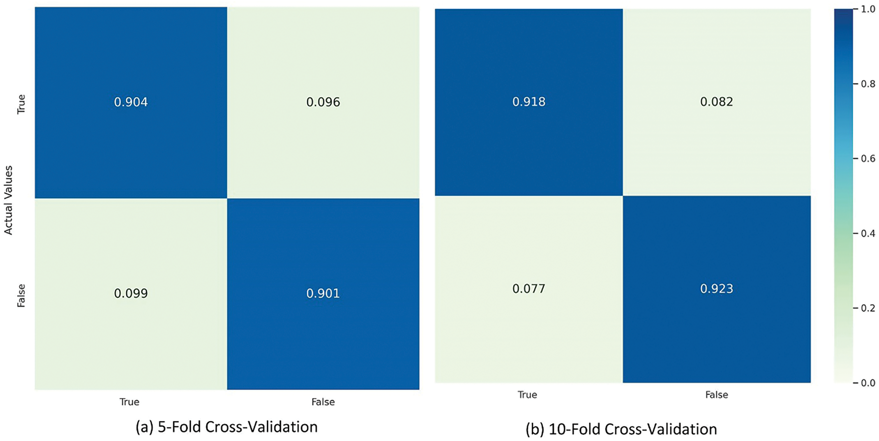
Figure 5: XGBoost confusion matrix using optimal hybrid features

4.4 Performance Comparison with Other Classifiers

Here, we use optimized hybrid feature vectors to compare the performance of the proposed model with other traditional ML classifiers. The classifiers being assessed, such as RF [20], SVM [21], NB, LR, and KNN [22]. Random Forest is a widely used ensemble learning technique for classification and prediction, constructing numerous decision trees from random data. SVM is extensively used in life sciences for linear and nonlinear classification since it identifies the optimal border for class separation [23]. Naive Bayes (NB) is a simple probabilistic classifier based on Bayes’ theorem, assuming feature independence. NB is widely used for text classification, spam detection, and medical diagnosis due to its efficiency and robustness. Logistic Regression (LR) is a statistical method used for binary classification, modeling the relationship between independent variables and a binary outcome using a sigmoid function. It is widely applied in healthcare, finance, and marketing for predictive analysis. KNN, often used in image processing, is a distance-based technique that classifies by contrasting instances. Table 7 presents a comparative analysis of the overall performance of several classifiers using 10-fold cross-validation.

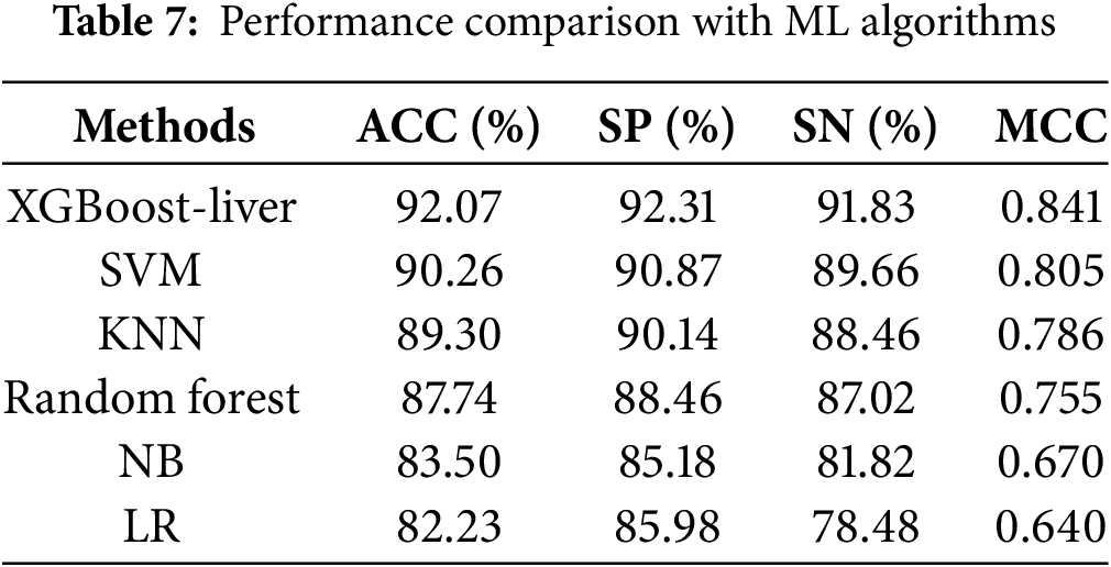
The proposed model achieved the highest accuracy of 92.07%, with an MCC of 0.841. Comparatively, among the traditional ML models, the SVM demonstrated an accuracy of 90.26%, a specificity of 90.87%, a sensitivity of 89.66%, and an MCC of 0.805. Similarly, the KNN and RF models achieve lower accuracy, at 89.30% and 87.74%, respectively, compared to XGBoost-Liver and SVM, highlighting limitations in managing complex data relationships and making them less suitable for datasets with mixed or overlapping classes. Overall, the XGBoost-Liver demonstrates the most balanced and robust performance, improving average accuracy by 2.96%. Furthermore, we compared the performance of the XGBoost-Liver model with traditional learning algorithms in terms of AUC (Area under the ROC curve) [24], as illustrated in Fig. 6. The ROC curve value indicates model efficiency, with higher values reflecting better performance. Fig. 6 highlights that the XGBoost-Liver model achieved the highest AUC of 0.932, outperforming SVM (0.912), KNN (0.902), and RF (0.881).

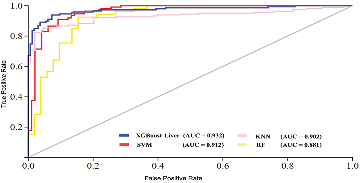
Figure 6: Area under the cure (AUC) performance comparison of machine learning algorithms

4.5 Performance Comparison with the Existing Predictors

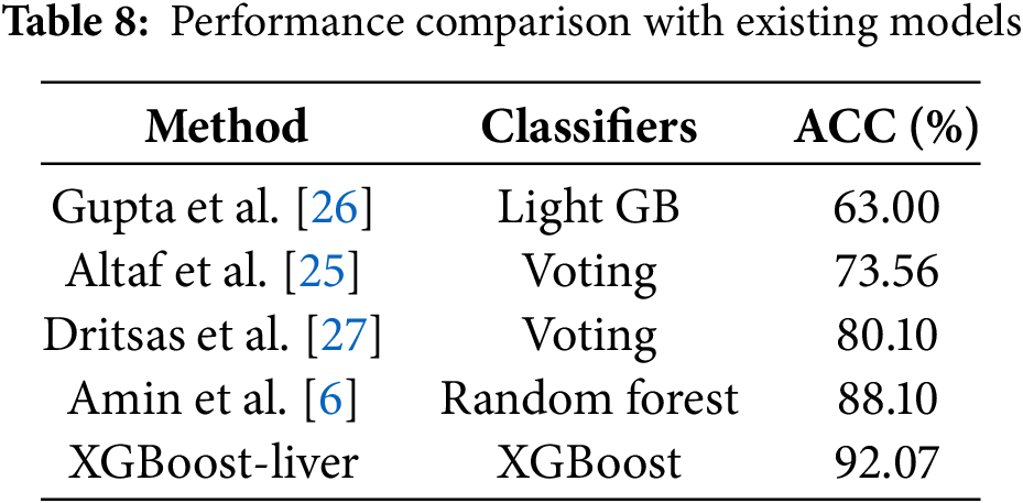
In this section, we compare the performance of the proposed model with the existing state-of-the-art models, as mentioned in [6,25–27]. Table 8 compares the proposed models with research published using the same dataset. Table 8 shows that the proposed model provided the best prediction accuracy among four previously published predictors. For example, Gupta et al. [26] in 2022 achieved an accuracy level of 63%, whereas the recently published predictor, Amin et al. [6], achieved an accuracy of 88.10%. Similarly, Dritsas et al. [27] achieved 80.10%. These results confirm that the proposed model performed better than the existing predictors, with an average accuracy improvement of 15.88%.

5  Conclusion

Liver disease (LD) is a severe condition that poses significant risks to human health and requires timely medical intervention. Healthcare professionals rely on neurological techniques for evaluating and diagnosing affected individuals. In this paper, we explored the prediction of chronic LD using an XGBoost method enhanced with integrated and optimized features. Our model used several techniques to assess feature importance, including ANOVA CHI2, PCA, and LDA. We also employed the Fisher score method to interpret complex features and select the most relevant ones for accurate LD prediction. The proposed XGBoost-Liver model underwent comprehensive performance evaluation, with experimental findings demonstrating its accuracy in predicting LD. Furthermore, a comparative analysis was conducted against existing models, revealing that the XGBoost-Liver model achieved superior performance compared to the alternatives.

Furthermore, the results show that our model enhances discriminative ability, offering a more reliable tool for the early detection of chronic LD. Integrating AI and machine learning into clinical settings holds great potential for advancing disease detection and improving patient outcomes. We plan to create an accessible web platform for biologists to use this model. Additionally, we aim to expand the dataset, explore new features, and implement more advanced algorithms to refine further and validate our model’s predictive capabilities.

Acknowledgement: The authors thank all the editors and anonymous reviewers for their comments and suggestions.

Funding Statement: This work was supported by Research Supporting Project Number (RSPD2025R585), King Saud University, Riyadh, Saudi Arabia.

Author Contributions: Salman Khan and Sumaiya Noor wrote the main manuscript text, Salman A. AlQahtani debugged the code, provided datasets, and reviewed the paper for grammar. All authors reviewed the results and approved the final version of the manuscript.

Availability of Data and Materials: The datasets used and analyzed during the current study are known as the ILPD dataset and are available in [6], as mentioned in our manuscript dataset.

Ethics Approval: Not applicable.

Conflicts of Interest: The authors declare no conflict of interest to report regarding the present study.

References

1. Prasad Babu MS, Ramjee M, Katta S, Swapna K. Implementation of partitional clustering on ILPD dataset to predict liver disorders. In: 2016 7th IEEE International Conference on Software Engineering and Service Science (ICSESS); 2016 Aug 26–28; Beijing, China: IEEE; 2016. p. 1094–7. doi:10.1109/ICSESS.2016.7883256. [Google Scholar] [CrossRef]

2. Gan D, Shen J, An B, Xu M, Liu N. Integrating TANBN with cost sensitive classification algorithm for imbalanced data in medical diagnosis. Comput Ind Eng. 2020;140:106266. doi:10.1016/j.cie.2019.106266. [Google Scholar] [CrossRef]

3. Anagaw A, Chang YL. A new complement Naïve Bayesian approach for biomedical data classification. J Ambient Intell Humaniz Comput. 2019;10(10):3889–97. doi:10.1007/s12652-018-1160-1. [Google Scholar] [CrossRef]

4. Sreejith S, Khanna Nehemiah H, Kannan A. Clinical data classification using an enhanced SMOTE and chaotic evolutionary feature selection. Comput Biol Med. 2020;126:103991. doi:10.1016/j.compbiomed.2020.103991. [Google Scholar] [PubMed] [CrossRef]

5. Kuzhippallil MA, Joseph C, Kannan A. Comparative analysis of machine learning techniques for Indian liver disease patients. In: 2020 6th International Conference on Advanced Computing and Communication Systems (ICACCS); 2020 Mar 6–7; Coimbatore, India: IEEE; 2020. p. 778–82. doi:10.1109/icaccs48705.2020.9074368. [Google Scholar] [CrossRef]

6. Amin R, Yasmin R, Ruhi S, Rahman MH, Reza MS. Prediction of chronic liver disease patients using integrated projection based statistical feature extraction with machine learning algorithms. Inform Med Unlocked. 2023;36(1):101155. doi:10.1016/j.imu.2022.101155. [Google Scholar] [CrossRef]

7. Khan S, AlQahtani SA, Noor S, Ahmad N. PSSM-Sumo: deep learning based intelligent model for prediction of sumoylation sites using discriminative features. BMC Bioinform. 2024;25(1):284. doi:10.1186/s12859-024-05917-0. [Google Scholar] [PubMed] [CrossRef]

8. Jain D, Singh V. Feature selection and classification systems for chronic disease prediction: a review. Egypt Inform J. 2018;19(3):179–89. doi:10.1016/j.eij.2018.03.002. [Google Scholar] [CrossRef]

9. Khan S, Khan M, Iqbal N, Dilshad N, Almufareh MF, Alsubaie N. Enhancing sumoylation site prediction: a deep neural network with discriminative features. Life. 2023;13(11):2153. doi:10.3390/life13112153. [Google Scholar] [PubMed] [CrossRef]

10. Khan S, Naeem M, Qiyas M. Deep intelligent predictive model for the identification of diabetes. AIMS Math. 2023;8(7):16446–62. doi:10.3934/math.2023840. [Google Scholar] [CrossRef]

11. Lu J, Kerns RT, Peddada SD, Bushel PR. Principal component analysis-based filtering improves detection for Affymetrix gene expression arrays. Nucleic Acids Res. 2011;39(13):e86. doi:10.1093/nar/gkr241. [Google Scholar] [PubMed] [CrossRef]

12. Raza A, Uddin J, Akbar S, Alarfaj FK, Zou Q, Ahmad A. Comprehensive analysis of computational methods for predicting anti-inflammatory peptides. Arch Comput Meth Eng. 2024;31(6):3211–29. doi:10.1007/s11831-024-10078-7. [Google Scholar] [CrossRef]

13. Rukh G, Akbar S, Rehman G, Alarfaj FK, Zou Q. StackedEnC-AOP: prediction of antioxidant proteins using transform evolutionary and sequential features based multi-scale vector with stacked ensemble learning. BMC Bioinform. 2024;25(1):256. doi:10.1186/s12859-024-05884-6. [Google Scholar] [PubMed] [CrossRef]

14. Chen J, Liu H, Yang J, Chou KC. Prediction of linear B-cell epitopes using amino acid pair antigenicity scale. Amino Acids. 2007;33(3):423–8. doi:10.1007/s00726-006-0485-9. [Google Scholar] [PubMed] [CrossRef]

15. Khan S, Khan MA, Khan M, Iqbal N, AlQahtani SA, Al-Rakhami MS, et al. Optimized feature learning for anti-inflammatory peptide prediction using parallel distributed computing. Appl Sci. 2023;13(12):7059. doi:10.3390/app13127059. [Google Scholar] [CrossRef]

16. Khan S, Khan M, Iqbal N, Rahman MAA, Karim MKA. Deep-piRNA: bi-layered prediction model for piwi-interacting RNA using discriminative features. Comput Mater Contin. 2022;72(2):2243–58. doi:10.32604/cmc.2022.022901. [Google Scholar] [CrossRef]

17. Bibi N, Khan M, Khan S, Noor S, AlQahtani SA, Ali A, et al. Sequence-based intelligent model for identification of tumor T cell antigens using fusion features. IEEE Access. 2024;12:155040–51. doi:10.1109/ACCESS.2024.3481244. [Google Scholar] [CrossRef]

18. Raza A, Uddin J, Zou Q, Akbar S, Alghamdi W, Liu R. AIPs-DeepEnC-GA: predicting anti-inflammatory peptides using embedded evolutionary and sequential feature integration with genetic algorithm based deep ensemble model. Chemometr Intell Lab Syst. 2024;254(377):105239. doi:10.1016/j.chemolab.2024.105239. [Google Scholar] [CrossRef]

19. Akbar S, Ullah M, Raza A, Zou Q, Alghamdi W. DeepAIPs-pred: predicting anti-inflammatory peptides using local evolutionary transformation images and structural embedding-based optimal descriptors with self-normalized BiTCNs. J Chem Inf Model. 2024;64(24):9609–25. doi:10.1021/acs.jcim.4c01758. [Google Scholar] [PubMed] [CrossRef]

20. Fawagreh K, Gaber MM, Elyan E. Random forests: from early developments to recent advancements. Syst Sci Contr Eng. 2014;2(1):602–9. doi:10.1080/21642583.2014.956265. [Google Scholar] [CrossRef]

21. Yue S, Li P, Hao P. SVM classification: its contents and challenges. Appl Math A J Chin Univ. 2003;18(3):332–42. doi:10.1007/s11766-003-0059-5. [Google Scholar] [CrossRef]

22. Cheng D, Zhang S, Deng Z, Zhu Y, Zong M. kNN algorithm with data-driven k value. In: Advanced data mining and applications. Cham: Springer; 2014. p. 499–512. [Google Scholar]

23. Khan S, Uddin I, Khan M, Iqbal N, Alshanbari HM, Ahmad B, et al. Sequence based model using deep neural network and hybrid features for identification of 5-hydroxymethylcytosine modification. Sci Rep. 2024;14(1):9116. doi:10.1038/s41598-024-59777-y. [Google Scholar] [PubMed] [CrossRef]

24. Basit A, Fawwad A, Qureshi H, Shera AS, Members NDSP. Prevalence of diabetes, pre-diabetes and associated risk factors: second national diabetes survey of Pakistan (NDSP2016–2017. BMJ Open. 2018;8(8):e020961. doi:10.1136/bmjopen-2017-020961. [Google Scholar] [PubMed] [CrossRef]

25. Altaf I, Butt MA, Zaman M. Hard voting meta classifier for disease diagnosis using mean decrease in impurity for tree models. Rev Comput Eng Res. 2022;9(2):71–82. doi:10.18488/76.v9i2.3037. [Google Scholar] [CrossRef]

26. Gupta K, Jiwani N, Afreen N, Divyarani D. Liver disease prediction using machine learning classification techniques. In: 2022 IEEE 11th International Conference on Communication Systems and Network Technologies (CSNT); 2022 Apr 23–24; Indore, India: IEEE; 2022. p. 221–6. doi:10.1109/CSNT54456.2022.9787574. [Google Scholar] [CrossRef]

27. Dritsas E, Trigka M. Supervised machine learning models for liver disease risk prediction. Computers. 2023;12(1):19. doi:10.3390/computers12010019. [Google Scholar] [CrossRef]