Data Aggregation Point Placement and Subnetwork Optimization for Smart Grids

Tien-Wen Sung; Wei Li; Chao-Yang Lee; Yuzhen Chen; Qingjun Fang

doi:10.32604/cmc.2025.061694

icon Open Access

ARTICLE

Data Aggregation Point Placement and Subnetwork Optimization for Smart Grids

Tien-Wen Sung¹, Wei Li¹, Chao-Yang Lee^2,*, Yuzhen Chen¹, Qingjun Fang¹

1 Fujian Provincial Key Laboratory of Big Data Mining and Applications, College of Computer Science and Mathematics, Fujian University of Technology, Fuzhou, 350118, China
2 Department of Computer Science and Information Engineering, National Yunlin University of Science and Technology, Yunlin, 640301, Taiwan

* Corresponding Author: Chao-Yang Lee. Email: email

(This article belongs to the Special Issue: Heuristic Algorithms for Optimizing Network Technologies: Innovations and Applications)

Computers, Materials & Continua 2025, 83(1), 407-434. https://doi.org/10.32604/cmc.2025.061694

Received 30 November 2024; Accepted 17 February 2025; Issue published 26 March 2025

Abstract

To transmit customer power data collected by smart meters (SMs) to utility companies, data must first be transmitted to the corresponding data aggregation point (DAP) of the SM. The number of DAPs installed and the installation location greatly impact the whole network. For the traditional DAP placement algorithm, the number of DAPs must be set in advance, but determining the best number of DAPs is difficult, which undoubtedly reduces the overall performance of the network. Moreover, the excessive gap between the loads of different DAPs is also an important factor affecting the quality of the network. To address the above problems, this paper proposes a DAP placement algorithm, APSSA, based on the improved affinity propagation (AP) algorithm and sparrow search (SSA) algorithm, which can select the appropriate number of DAPs to be installed and the corresponding installation locations according to the number of SMs and their distribution locations in different environments. The algorithm adds an allocation mechanism to optimize the subnetwork in the SSA. APSSA is evaluated under three different areas and compared with other DAP placement algorithms. The experimental results validated that the method in this paper can reduce the network cost, shorten the average transmission distance, and reduce the load gap.

Keywords

Smart grid; data aggregation point placement; network cost; average transmission distance; load gap

1 Introduction

The growing development of communication technology provides power grids with the means to effectively control and monitor power information [1]. A smart grid is the transformation of a power grid from a traditional electromechanical control system to an electronic control network [2]. Smart grids are based on an integrated, fast bidirectional communication network. Through the application of advanced sensing and measuring technologies, control means, and decision-making system technologies, they realize the goals of economic, high-efficiency, and environmental friendliness in the use of power grids [3].

An infrastructure that allows for bidirectional communication is called an advanced metering infrastructure (AMI) and is considered an essential component of smart grids. It consists of a smart meter (SM) installed at a customer’s end, a metering data management system located in the utility company, and a communication system connecting both, constituting a complete network processing system for measuring, collecting, processing, and utilizing customers’ electricity consumption information [4]. AMI employs a stationary bidirectional communication network that reads the SM several times a day and transmits meter information, including fault alarms, to the data control center in near real-time [5,6].

AMI consists of three main categories: home area network (HAN), neighborhood area network (NAN), and wide area network (WAN). HAN is the network within a user’s home or premises, which includes SM and other smart devices that collect power information from the users. NAN serves as an intermediate network between HAN and WAN. In NAN, data collected from HAN devices are transmitted to WAN for further processing and analysis. WAN is responsible for connecting multiple WANs and further transmitting the collected user power data to the control center or data management system. To enable communication within these networks, various technologies are commonly used. ZigBee, WiFi, Bluetooth, power line communication, and 5G are among the preferred technologies for AMI networks [7,8]. A visual representation of the AMI network framework is shown in Fig. 1.

images

Figure 1: AMI network framework diagram

NAN is an important part of a smart grid communication network. It usually consists of an SM and a data aggregation point (DAP). DAP collects power information from different SMs and forwards it to the WAN gateway. Wireless communication is recommended for NAN because of its low cost, ability to connect a large number of devices, and ease of deployment [9–11]. In NAN, the location of DAPs and the number of installations significantly impact the quality of communication between DAPs and SMs. First, the position of the DAP affects the transmission distance between the DAP and SM, thereby influencing the power consumption and transmission rate of NAN. Second, the number of DAPs affects the operational costs of NAN; therefore, an appropriate number of DAPs must be selected while ensuring sufficient network coverage [12]. Finally, each DAP has its maximum load; thus, if too many SMs are connected to a DAP, it not only overloads the DAP but also causes a delay in transmitting data from the DAP to the control center [13].

However, the problems in selecting the number of DAPs to be installed in the NAN and the location of the installations (the DAP placement problem) have not been well explored. In this paper, we investigate the placement of DAPs in NANs with different numbers of SMs (urban, suburban, and rural) to determine the appropriate number of DAPs to reduce the operational cost of a NAN, select appropriate locations for DAP placement to minimize the average transmission distance between SMs and DAPs, and optimize subnetworks to minimize the gap in the number of loads between different DAPs. The simulated experimental results demonstrate that our proposed affinity propagation (AP) algorithm and sparrow search (SSA) (APSSA) algorithm can select the appropriate number of DAPs to reduce the network cost of NANs, shorten the average transmission distance between SMs and DAPs, and reduce the load gap of DAPs.

The main contributions of this paper are as follows:

(1) This study improves the AP algorithm so that it can arrive at an optimal number of DAP installations and installation locations on the basis of the number and distribution of SMs in different environments without the need to preset the number of DAP installations while reducing the average transmission distance.

(2) In this paper, we consider optimizing different subnetworks as a set covering problem (SCP) and establish corresponding coverage matrices to better solve the subnetwork optimization problem to reduce the load gap between different DAPs.

(3) Based on the initial DAP and its corresponding subnetwork, the SSA algorithm is used to optimize the subnetwork. An allocation mechanism is added to the SSA algorithm to allocate SM-optimized subnetworks to reduce the load gap and form the final subnetwork.

(4) The APSSA algorithm is comprehensively evaluated considering three different NAN regions.

The rest of the paper is organized as follows: Section 2 discusses related work. Section 3 describes the network model and the network cost model. In Section 4, the APSSA algorithm proposed in this paper is described in detail. The performance of the APSSA algorithm in simulation experiments is described in detail in Section 5. Section 6 concludes the paper and presents our future research directions.

2 Related Work

The number and placement of DAPs in a network play a vital role in wireless communication between SMs and DAPs [14]. In this regard, Li et al. [15] introduced an effective approximation algorithm to handle smart grid communication optimization tasks, which can handle complex DAP planning tasks and help reduce the costs of smart grid communication systems. Meanwhile, Gallardo et al. [16] proposed a DAP optimization framework based on residential grid AMI using K-medoids to select the optimal placement of DAPs. Their experimental results demonstrated that their method could reduce the average and maximum distance of communication between SMs and DAPs to some extent. In another study, Kong [13] argued that in a smart grid, the communication network and the power network are interdependent; thus, the DAP placement problem cannot be considered as a communication network problem only. Kong [17] further argued that in a smart grid where power is supplied to DAPs by a transformer, the failure of the transformer results in the loss of power to the corresponding connected DAPs and the loss of monitoring function, which in turn results in the failure of the network cascade. Therefore, the DAP placement problem must also fully consider how an SM can communicate normally with the data control center after a failure of the transformer or DAP in a network.

The continuous development of Internet of Things (IoT) technologies provides new opportunities and motivation for different smart grid applications, such as AMI and electric vehicles [18–20]. The development of artificial intelligence IoT [21,22] has accelerated this process. In this respect, Gallardo et al. [23] proposed an IoT-based AMI architecture that consists of three layers: a sensing layer, a communication network layer, and an application layer. Meanwhile, Khan et al. [24] proposed a quality of service (QoS)-based machine learning framework for AMI to better design efficient smart grid architectures. This proposed framework consisted of three components: a three-tier hierarchical architecture for AMI, a hierarchical clustering approach based on machine learning, and a scheduling technique based on application item prioritization. However, integrating these technologies has also introduced new security challenges, particularly the vulnerability of machine learning-based smart grid applications (MLsgAPPs) to malicious attacks. Zhang et al. [25] provided a comprehensive review of recent advances in attack strategies and defense mechanisms for MLsgAPP security, marking a significant contribution as the first overview in this domain. This study extends the discussion by systematically reviewing and comparing existing research on adversarial attacks in MLsgAPP across power generation, transmission, distribution, and consumption scenarios, while also examining countermeasures. Additionally, it analyzes potential vulnerabilities in smart grid applications powered by large language models (e.g., ChatGPT). Literature [26] investigated data security risks in ML-based smart grids, focusing on adversarial manipulations of critical input systems that could mislead system operators and trigger cascading failures, such as major power outages. To address this issue, this study proposes a physics-constrained robustness evaluation framework based on the tree ensemble (TE) model, ensuring that adversarial samples not only deceive human intuition but also comply with physical laws and bypass the power system’s error-checking mechanisms. By employing formal modeling and variable transformation, an effective robustness assessment method is introduced and validated through simulations.

Artificial intelligence techniques can be applied to meet QoS requirements when determining the placement of selected DAPs for a communication network structure, especially in some urban areas with a high density of meter coverage. In particular, clustering methods [27] are useful for solving this optimization problem [28]. Hassan et al. [29] evaluated and compared three clustering algorithms, namely, K-means, self-organizing map, and fuzzy c-means, for the DAP placement problem in terms of the multihop shortest path distance, cluster size, and computational complexity. Their simulation results showed that allocation methods based on the K-means and self-organizing map had similar performances, whereas that based on fuzzy c-means had a longer maximum multihop shortest path distance and higher complexity. Molokomme et al. [30] proposed a NAN layout scheme based on an unsupervised K-means clustering algorithm and a silhouette index method.

Other previous studies [31,32] presented a new idea of selecting SMs to work as DAPs directly in the NAN. They concluded that shortening the transmission distance path between SMs and DAPs is an important initiative to reduce the energy and time cost of a network in a smart grid communication network environment. Thus, they categorized the DAP placement problem as solving the shortest distance path problem and proposed the algorithms and using a multihop communication model to reduce the number of DAPs. Table 1 shows the brief summary of the major related works.

images

In smart grids, large amounts of data must be processed and exchanged. The availability of smart grids requires meeting time delays for different operations and data transmission [33]. The shortest transmission path is one of the commonly used approaches in various DAP placement problems as it provides an effective way to reduce the consumption of network energy and the time taken to transmit data. In DAP placement problems, the number of DAPs and their location selection is a very critical issue. In current research, most clustering algorithms with an initial predetermined number of DAPs are used for the location selection of DAPs. However, determining how many DAPs are optimal is difficult, especially for such a large network as a smart grid. Moreover, the number of SMs connected by DAPs is not considered, which may easily lead to a large gap between the number of SMs connected by different DAPs in the network, which is not conducive to the distribution of energy and the guarantee of communication quality of the smart grid. Therefore, in this paper, we focus on automatically selecting the appropriate number of SMs as DAPs from all the SMs in the NAN without presetting the number of DAPs, thereby reducing the network costs, minimizing the average transmission distance between SMs and DAPs, and balancing the load volume gap between different DAPs.

3 System Modeling and Problem Formulation

3.1 NAN Model

In this study, SM and DAP are connected using wireless communication. SM can send the data directly to the DAP or it can also be used as a relay for forwarding the data from other SMs to the DAP, as shown in Fig. 2.

images

Figure 2: NAN model

There are N smart meters $S M = {s m_{i} ∣ i = 1, 2, \dots, N}$ $SM={smi∣i=1,2,…,N}$ randomly distributed in the $L \times W$ $L×W$ region monitored by NAN, and setting different numbers of $S M s N$ $SMsN$ in the region can change the distribution density of $S M s ρ_{S M}$ $SMsρSM$ , $N = ρ_{S M} \cdot (L \cdot W)$ $N=ρSM⋅(L⋅W)$ . All $S M s$ $SMs$ have the same transmission range, which is denoted by a circle of radius $r_{c}$ $rc$ meters. Let $(x_{i}, y_{i})$ $(xi,yi)$ denote the coordinates of the $i$ $i$ th $S M s m_{i}$ $SMsmi$ . The distance between any two $S M s s m_{i}$ $SMssmi$ and $s m_{j}$ $smj$ is denoted by:

$d (s m_{i}, s m_{j}) = \sqrt{(x_{i} - x_{j})^{2} + (y_{i} - y_{j})^{2}}$ $d(smi,smj)=(xi−xj)2+(yi−yj)2$ (1)

If $d (s m_{i}, s m_{j}) \leq r_{c}$ $d(smi,smj)≤rc$ , the two $S M s$ $SMs$ are considered neighboring and can be connected directly. The shortest transmission distance between the neighboring $S M s s m_{i}$ $SMssmi$ and $s m_{j}$ $smj$ is $d i s t a n c e (s m_{i}, s m_{j}) = d (s m_{i}, s m_{j})$ $distance(smi,smj)=d(smi,smj)$ , and the path is $r o u t e (s m_{i}, s m_{j}) = s m_{j}$ $route(smi,smj)=smj$ . The $r o u t e (s m_{i}, s m_{j})$ $route(smi,smj)$ indicates which node is the next step from $s m_{i}$ $smi$ to $s m_{j}$ $smj$ . If $d (s m_{i}, s m_{j}) > r_{c}$ $d(smi,smj)>rc$ , then these two $S M s$ $SMs$ are considered nonadjacent. The shortest transmission distance and path between nonadjacent $S M s s m_{i}$ $SMssmi$ and $s m_{j}$ $smj$ must be obtained by searching the entire network using the Floyd-Warshall algorithm. The neighbor nodes of $S M s m_{i}$ $SMsmi$ are denoted as $φ (s m_{i})$ $φ(smi)$ and defined as all $S M s$ $SMs$ within the communication range $r_{c}$ $rc$ of $s m_{i}$ $smi$ . That is:

$φ (s m_{i}) = {s m_{j} ∣ d (s m_{i}, s m_{j}) \leq r_{c}, s m_{j} \in S M}$ $φ(smi)={smj∣d(smi,smj)≤rc,smj∈SM}$ (2)

The whole network is connected, which means that any two different SMs can directly or indirectly, through a limited number of relay SMs, communicate with each other. In this paper, the DAP placement task is to select a certain number of SMs from the NAN as DAPs and assign other SMs to these DAPs, dividing the whole NAN into different subnetworks. Each subnetwork has only one DAP, and these DAPs collect the data collected by the SMs within their own subnetwork to be forwarded to the WAN after further processing. The DAP can be denoted as:

$D A P S = {D A P_{1}, D A P_{2}, D A P_{3}, \dots, D A P_{τ}}$ $DAPS={DAP1,DAP2,DAP3,…,DAPτ}$ (3)

where $τ$ $τ$ is the number of subnetworks which is also the number of DAPs. Each subnetwork can be represented as:

$S N S = {S N_{1}, S N_{2}, S N_{3}, \dots, S N_{τ}}$ $SNS={SN1,SN2,SN3,…,SNτ}$ (4)

$S N_{i}$ $SNi$ denotes the set of SMs communicating with $D A P_{i}$ $DAPi$ , $S N_{i} = {s_{1}, s_{2}, s_{3}, \dots, s_{n_{i}}}$ $SNi={s1,s2,s3,…,sni}$ , where $n_{i} = | S N_{i} |$ $ni=|SNi|$ denotes the number of SMs communicating with $D A P_{i}$ $DAPi$ , and the load volume $L o a d (D A P_{i}) = n_{i}$ $Load(DAPi)=ni$ . The average transmission distance $D_{a v g}$ $Davg$ between a DAP and its connected SMs is denoted as follows:

$D_{a v g} = \frac{\sum_{j = 1}^{τ} \sum_{s m_{i} \in S N_{j}} d i s t a n c e (s m_{i}, D A P_{j})}{\sum_{j = 1}^{τ} n_{j}}$ $Davg=∑j=1τ∑smi∈SNjdistance(smi,DAPj)∑j=1τnj$ (5)

To better measure the load gap of different DAPs, we use the population standard deviation to measure the load gap of different subnetworks in the whole network, denoted as follows:

$L = \sqrt{\frac{\sum_{i = 1}^{τ} (L o a d (D A P_{i}) - ¯ ¯¯¯¯¯¯¯¯¯¯ ¯ L o a d)^{2}}{τ}}$ $L=∑i=1τ(Load(DAPi)−Load¯)2τ$ (6)

In this equation, L is the load gap and $¯ ¯¯¯¯¯¯¯¯¯¯ ¯ L o a d$ $Load¯$ is the average load.

3.2 Network Cost Model

The total cost of the network can be categorized into three parts: DAP installation and maintenance cost $c_{m a i n}$ $cmain$ , data transmission cost $c_{t r a n s}$ $ctrans$ , and delay cost $c_{d l y}$ $cdly$ [34]. Therefore, the sum of these costs should be minimized when selecting the placement of DAPs:

$c_{t o t a l} = c_{m a i n} + c_{t r a n s} + c_{d l y}$ $ctotal=cmain+ctrans+cdly$ (7)

Although SMs are selected from the network as DAPs, ordinary SMs cannot process large amounts of data. Thus, to meet the network needs, a device that can process large amounts of data has to be installed as a DAP at the location of the original SM. The cost of installing and maintaining a DAP is A. Then, $c_{m a i n}$ $cmain$ is proportional to the number of DAPs selected to be set up and is denoted as:

$c_{m a i n} = A \cdot τ$ $cmain=A⋅τ$ (8)

$c_{t r a n s}$ $ctrans$ denotes the average power cost consumed over the entire network lifetime for the transmission of collected power data from SM to the relay SM or directly from SM to DAP, denoted as:

$c_{t r a n s} = B \sum_{i = 1}^{N} \sum_{j = 1}^{N} y_{i j} \cdot P L (d i s t a n c e (s m_{i}, s m_{j}))$ $ctrans=B∑i=1N∑j=1Nyij⋅PL(distance(smi,smj))$ (9)

where $y_{i j}$ $yij$ is a binary variable; $y_{i j}$ $yij$ is 1 if $s m_{i}$ $smi$ is assumed to communicate directly with $s m_{j}$ $smj$ , and 0 if it is not. N is the number of SMs in the network. $B = g 8 M γ E_{b} κ T_{m} / T_{l}$ $B=g8MγEbκTm/Tl$ is the transmission cost per SM per unit of path loss; $T_{l}$ $Tl$ is the time interval between the transmissions; $T_{m}$ $Tm$ is the assumed lifetime of the network; $g$ $g$ is the price of energy; $γ$ $γ$ is the ratio of the total modeled power consumption to the transmission power; $E_{b}$ $Eb$ is the required received energy per bit; $κ$ $κ$ is the fading margin; and the factor 8 in the formula indicates that M is the packet size in bytes. For more detailed information on these parameters, see previous works in the literature [12,34]. In this paper, we select some of these SMs as DAPs among the SMs present in the NAN. Therefore, assuming that $s m_{i}$ $smi$ is selected as a DAP, we can denote this DAP with the original coordinate $(x_{i}, y_{i})$ $(xi,yi)$ . $P L (d i s t a n c e (s m_{i}, s m_{j}))$ $PL(distance(smi,smj))$ is the desired path loss over the communication distance $d i s t a n c e (s m_{i}, s m_{j})$ $distance(smi,smj)$ between SM $s m_{i}$ $smi$ and $s m_{j}$ $smj$ , denoted as follows:

$P L (d i s t a n c e (s m_{i}, s m_{j})) = P L_{d_{0}} \cdot {(\frac{d i s t a n c e (s m_{i}, s m_{j})}{d_{0}})}^{ω}, i, j = 1, 2, \dots, N$ $PL(distance(smi,smj))=PLd0⋅(distance(smi,smj)d0)ω,i,j=1,2,…,N$ (10)

$P L_{d_{0}}$ $PLd0$ is the path loss at the reference distance $d_{0}$ $d0$ , and $ω$ $ω$ is the path-loss exponent. The delay cost $c_{d l y}$ $cdly$ can be expressed as:

$c_{d l y} = C \cdot h o p (s m_{i}, D A P_{j}), s m_{i} \in S N_{j}, j = 1, 2, \dots, τ$ $cdly=C⋅hop(smi,DAPj),smi∈SNj,j=1,2,…,τ$ (11)

$h o p (s m_{i}, D A P_{j})$ $hop(smi,DAPj)$ is denoted as the number of hops between $s m_{i}$ $smi$ and its communicating $D A P_{j}$ $DAPj$ . C is the delay cost, which is the loss in the number of hops of the path connecting the sender SM to its corresponding DAP. Introducing the coefficient C transforms the communication delay into a monetary loss [34].

3.3 Problem Formulation

The main objective of this paper is to select the best SM as a DAP among the SMs distributed in the NAN and to divide the NAN into various subnetworks to shorten the average transmission distance between the SMs and their belonging DAPs, reduce the load gap of each DAP, and reduce the cost of the network. The DAP placement problem is formulated as:

$minDavg$ (12)

$minL$ (13)

$minctotal$ (14)

The constraints are as follows:

$⋃i=1τSNi=SM$ (15)

$SNi∩SNj=∅∀i≠j,i,j=1,2,…,τ$ (16)

$SNi is a network of connections∀i=1,2,…,τ$ (17)

$DAPi∈SM∀i=1,2,…,τ$ (18)

Constraint (15) denotes that all SMs are covered by the subnetwork. Constraint (16) denotes that there is no duplicate coverage of SMs between different subnetworks; that is,each SM can only be assigned to a single subnetwork. Constraint (17) denotes that SMs within each subnetwork can be transmitted either directly or through a limited number of relay meters, and that the entire subnetwork is a connected network. Constraint (18) indicates that the placement of the DAP is the location of the original SM, not a newly added location in the network.

4 The Proposed APSSA Algorithm

4.1 Selection of the Number and Location of DAPs to Form Initial Subnetworks

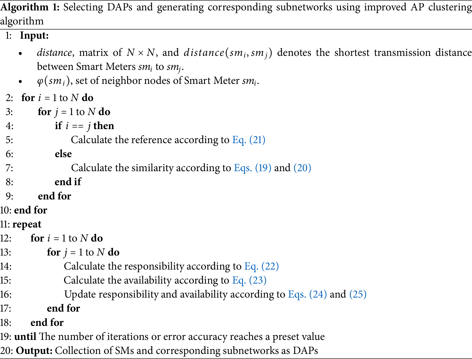
In APSSA the number of DAPs and their positions are selected to form an initial subnetwork based on the number of SMs and distribution positions using the improved AP clustering algorithm.

Traditional clustering algorithms such as K-means and K-medoids require a predefined number of cluster centers based on data characteristics, and their results are highly sensitive to the initial cluster values. To address these limitations, Frey and Dueck proposed the affinity propagation (AP) clustering algorithm in 2007. Compared with traditional methods, AP clustering offers greater adaptability and stability. The core idea of AP clustering is to establish a similarity matrix between data points and iteratively transfer information to determine the optimal data clusters. The AP clustering algorithm relies on three types of information: similarity, responsibility, and availability. During execution, the algorithm uses similarity information to guide clustering, while responsibility and availability information are iteratively updated to refine the clustering process, ultimately selecting the optimal clustering result.

This study enhances the AP clustering algorithm for wireless neighborhood area network (NAN) scenarios, enabling the adaptive determination of data aggregation points (DAPs) and their optimal placement based on smart meter (SM) quantity and distribution. The improved algorithm aims to minimize network interference and reduce the average transmission distance between SMs and their assigned DAPs.

To reduce the average transmission distance between SM and DAP, the similarity is calculated using the negative value of the shortest transmission distance $distance(smi,smj)$ between $smi$ and $smj$ and the average transmission distance from $smi$ to the other SMs, as shown in Eq. (19):

$s(smi,smj)=−distance(smi,smj)averageii,j∈{1,…,N} and i≠j$ (19)

where the average distance $averagei$ is shown in Eq. (20):

$averagei=∑j=1Ndistance(smi,smj)Ni,j∈{1,…,N} and i≠j$ (20)

The similarity $s(smi,smj)$ between $smi$ and $smj$ indicates the degree of suitability of $smj$ as a DAP for $smi$ . The diagonal element $s(smi,smi)$ of the similarity matrix represents the reference of $smi$ . The larger $s(smi,smi)$ is, the higher the probability of $smi$ being a DAP. The reference is calculated as shown in Eq. (21):

$s(smi,smi)=−Avgsmax(smi)−Avgsmin(smi)Avgs(smi)−Avgsmin(smi)⋅|φ(smi)|max|φ(smi)|⋅αi∈{1,…,N}$ (21)

$Avgs(smi)=∑j∈φ(smi)s(smi,smj)/|φ(smi)|$ denotes the average similarity of $smi$ . $Avgsmax(smi)$ and $Avgsmin(smi)$ respectively denote the maximum and minimum values of the average similarity among the neighboring nodes of $smi$ . $|φ(smi)|$ is the number of neighbor nodes of $smi$ . $|φ(smi)|max$ denotes the number of nodes with maximum neighbors among all the SMs of the NAN, and $α$ is the reference degree coefficient, which affects the reference degree of the SMs. The larger $α$ is, the smaller the reference degree of each SM and the smaller the number of DAPs in the network.

$r(smi,smj)=s(smi,smj)−maxj∗≠jj,j∗∈N{s(smi,smj∗)+a(smi∗,smj∗)}$ (22)

$a(smi,smj)={∑i∗≠ii∗∈Nmax{0,r(smi∗,smj)}if j=imin(0,r(smi,smj)+∑i∗∈Ni∗≠i,jmax{0,r(smi∗,smj)})if j≠i$ (23)

After determining the similarity $s(smi,smj)$ and the reference $s(smi,smj)$ , we utilize Eqs. (22) and (23) to compute and update the responsibility $r(smi,smj)$ and availability $a(smi,smj)$ . The algorithm is initialized by first presetting all the availability to 0. The responsibility $r(smi,smj)$ is sent from $smi$ to $smj$ , reflecting the extent to which $smj$ is suitable to serve as a DAP for $smi$ after considering the other SM as a DAP. $a(smi,smj)$ sends from $smj$ to $smi$ , reflecting the appropriateness of $smi$ choosing $smj$ as the DAP after considering the support of other SMs for $smj$ to be the DAP. The information transfer process is shown in Fig. 3.

images

Figure 3: The information of responsibility and availability

To avoid data oscillations during the iteration process, damping coefficients are set to update the values of responsibility and availability, as shown in Eqs. (24) and (25):

$rt+1(smi,smj)=λrt(smi,smj)+(1−λ)rt+1(smi,smj)$ (24)

$at+1(smi,smj)=λat(smi,smj)+(1−λ)at+1(smi,smj)$ (25)

$rt+1(smi,smj)$ and $at+1(smi,smj)$ respectively denote the values of responsibility and availability for the $t+1$ iteration, whereas $rt(smi,smj)$ and $at(smi,smj)$ respectively denote the values of responsibility and availability for the $t$ iteration. The iteration is terminated when the number of iterations or the error accuracy reaches a preset value. At the end of the iteration, for $smi$ , take $smj$ that maximizes $r(smi,smj)+a(smi,smj)$ . If $j=i$ , then $smi$ is selected as the DAP; otherwise, the meter node $smj$ is used as the DAP of $smi$ . According to this rule, the initial DAP can be selected and SM is assigned to the corresponding DAP to form the initial subnetwork. Algorithm 1 gives the pseudocode for the above description.

images

4.2 Optimization of Subnetworks Based on SSA Algorithm

In this section, the previously generated subnetworks are optimized to minimize the load gap among different DAPs. This study introduces the set coverage problem (SCP) models subnetwork optimization as an SCP problem. A distance threshold ( $β$ ) is incorporated in the algorithm to balance transmission distance and load distribution. Based on this threshold, a SM coverage matrix is generated. Next, the SSA algorithm is applied to solve the SCP problem in the subnetwork. Unlike the traditional SSA algorithm, this approach intergrates an allocation mechanism that reasonably assigns SMs based on the DAP selected by each individual, improving load balancing. By optimizing and improving the initial subnet structure formed by the AP algorithm, the proposed method effectively reduces the load gap among different DAPs.

4.2.1 SCP and Coverage Matrix

In the general SCP problem, assume that there is a set X consisting of $x$ elements and corresponding $y$ subsets $Cj⊆X$ , where $j={1,…,y}$ . The goal is to select multiple subsets so that each element in X belongs to at least one of these subsets while minimizing some sum of costs. In this paper, we hope to reduce the DAP load gap. To solve the SCP, a coverage matrix must first be constructed, as shown in Fig. 4, where the elements of the matrix are denoted by $Coverij$ , $D1$ and $D2$ denote DAP, and $SM1$ – $SM12$ denote SM. If $Coverij=1$ , it means that the $i$ th SM can connect with the $j$ th DAP. If $Cover11=1$ but $Cover12=0$ , it means that $SM1$ can only communicate with $D1$ . Notably, $SM5$ and $SM11$ can use $SM1$ as a relay node to communicate with $D1$ , even though they are out of range of $D1$ ’s communication.

images

Figure 4: Coverage matrix based on Smart Meter location

SCP has been proved to be an NP-hard problem. Therefore, in practice, some approximation algorithms, such as greedy algorithms or metaheuristic algorithms, are often used to find an approximate optimal solution [35,36].

4.2.2 Algorithm Steps

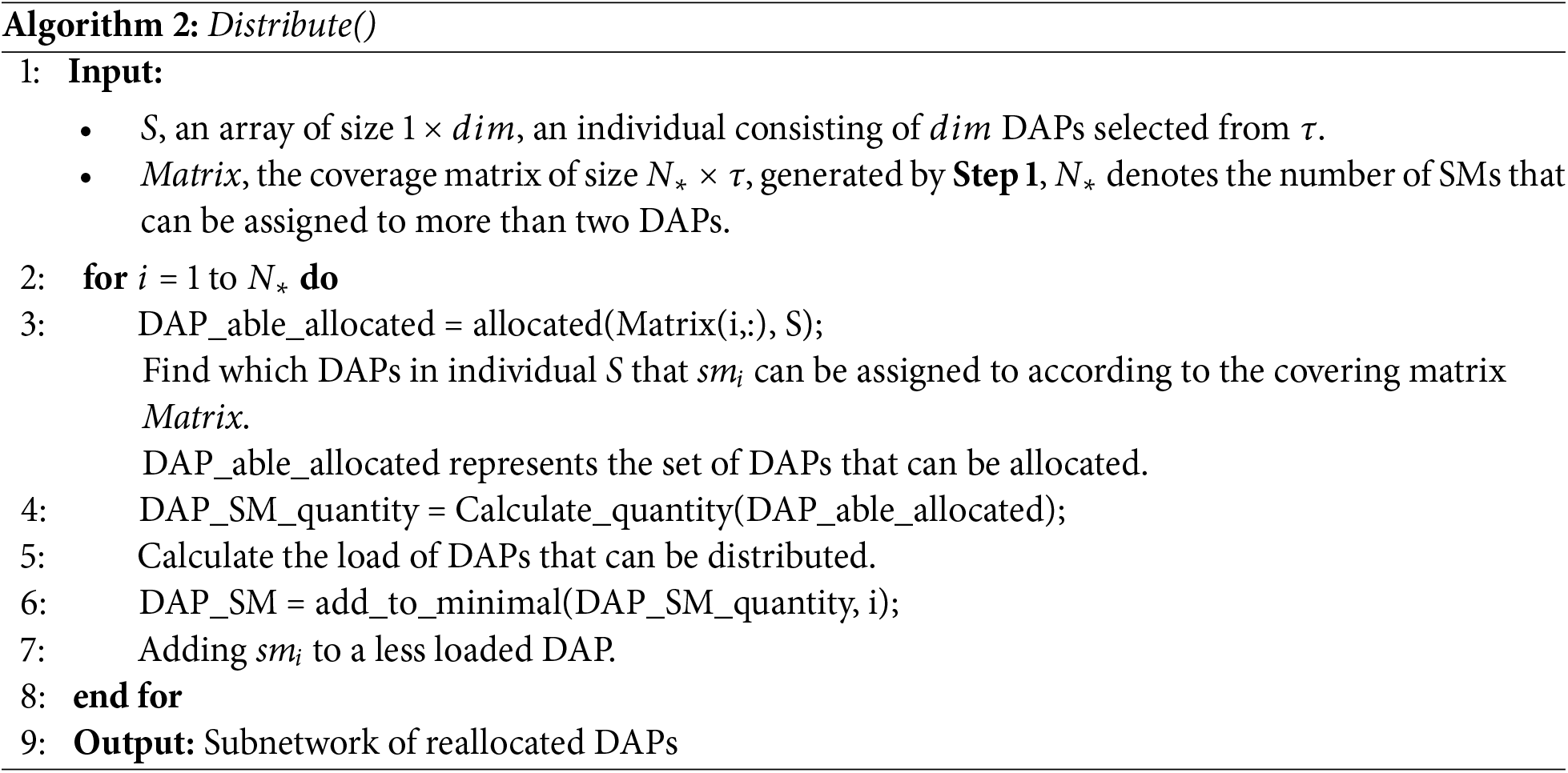
Step 1: In the initial subnetwork generated by the AP algorithm, the load gap between different DAPs is very large to allow SM to be assigned to other DAPs to reduce the load gap between different DAPs, to optimize the subnetwork and effectively reduce the average transmission distance. We set the distance threshold $β$ as shown in Eq. (26):

$coverij={1if distance(smi,DAPj)≤β⋅distance(smi,DAP∗)0if distance(smi,DAPj)>β⋅distance(smi,DAP∗)i=1,…,Nj=1,…,τ$ (26)

$coverij$ denotes the matrix element corresponding to the $i$ th SM $smi$ and the $j$ th DAP, and $DAP∗$ denotes the DAP to which $smi$ is connected in the initial subnetwork. We combine the SMs that can be assigned to more than two different DAPs into a coverage matrix, as shown in Fig. 5.

images

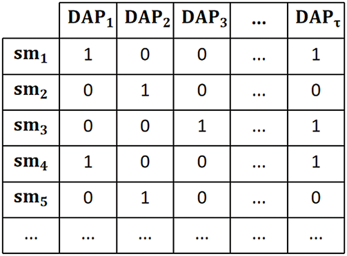
Figure 5: Constituent coverage matrix

Step 2: Initialize the population. The initial population is generated randomly by randomly selecting $dim$ DAPs out of $τ$ DAPs that constitute an individual S in the population, which also denotes the position of each individual, and the size of the population is $pop$ . In the algorithm, we add an allocation mechanism $Distribute$ to balance the amount of load between different DAPs. Algorithm 2 describes the mechanism.

images

Step 3: Calculate the fitness value of each individual in the population species, as shown in Eq. (27):

$fitness(S)=L=∑i=1τ(Load(DAPi)−Load¯)2τ$ (27)

Step 4: Update the position of the explorer. Calculate the fitness value of each individual in the population according to Step 3, and sort the population according to the fitness value. The top $Epercent$ individuals are the explorers, as shown in Eq. (28):

$Xi,jt+1={Xi,jt⋅exp(−iθ⋅itermax)if R2<STXi,jt+Q⋅pif R2≥ST$ (28)

where $Xijt$ represents the position information of the $i$ th individual in the explorer on the $j$ th in the $t$ th iteration, which is the $j$ th selected DAP. $θ$ is a random number in $[0,1]$ , $itermax$ is the maximum number of iterations,Q is a random number obeying a normal distribution, and $p$ is a $1×dim$ matrix with all ones. ST represents the safety threshold, and $R2$ is a random number in $[0,1]$ indicating the warning value. When $R2<ST$ , it means that the current location is safe; when $R2≥ST$ , it means that the current location is dangerous and the individual needs to move to a safe area. After the position of each explorer is updated, such position is restricted to within $τ$ . The Distribute allocation mechanism is utilized to assign the SM, and the fitness value of each explorer is then calculated.

Step 5: Update the location of the followers. In the population, all except explorers are followers. As shown in Eq. (29):

$Xi,jt+1={Q⋅exp(Xworstt−Xi,jti2)if i<Z/2Xpt+1+|Xi,jt−Xi,jt+1|⋅A+⋅potherwise$ (29)

where $Xworstt$ is the worst individual in the $t$ th iteration and $Xpt+1$ is the position of the current optimal explorer, $A+=AT(AAT)−1$ . When the $i$ th individual among the followers is the better follower of the first half, the position is updated using the first subequation; when that follower is the worse follower of the second half, it corresponds to the individual being very hungry and needing to randomly fly elsewhere in search of food. Z is the number of followers. After the position of each follower is updated, the position of each follower is restricted to within $τ$ . The Distribute allocation mechanism is utilized to assign the SM, and then the fitness value of each follower is calculated.

Step 6: Update the location of individuals aware of the danger. We randomly selected $Dpercent$ individuals from the population as individuals aware of the danger, as shown in Eq. (30):

$Xi,jt+1={Xbestt+ψ⋅|Xi,jt−Xbestt|if fi<fgXi,jt+k⋅(|Xi,jt−Xworstt|(fi−fw)+ε)if fi=fg$ (30)

where $Xbestt$ is the optimal individual in the $t$ th iteration, $ψ$ is a random number that obeys a normal distribution with a mean of 0 and a variance of 1, $k$ is a random number of $[−1,1]$ , $fi$ is the fitness value of the current individual, $fg$ is the current worst fitness value, and $ϵ$ is a constant that prevents the denominator from being 0 and is usually very small. After the location of each individual who is aware of the danger is updated, such location is limited to $τ$ . The Distribute allocation function is then used to allocate SM, and the fitness value of the individual who is aware of the danger is calculated.

Step 7: Judge whether the stopping condition is satisfied; if so, output the optimal sparrow individual position and the corresponding fitness value; otherwise, return to Step 4.

The detailed flowchart of APSSA is shown in Fig. 6.

images

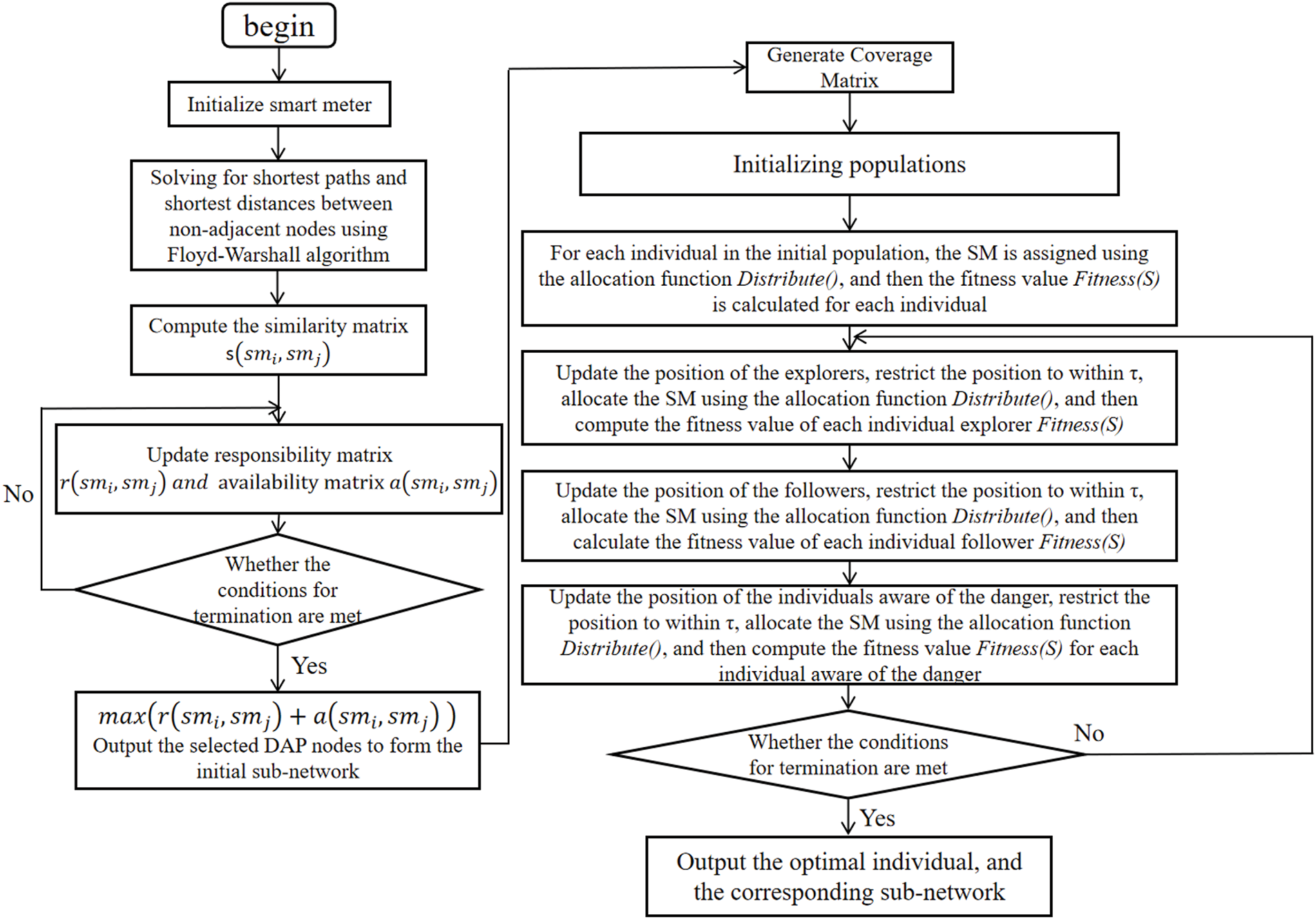
Figure 6: Algorithm flowchart

5 Performance Evaluation

Experiments were conducted by deploying varying numbers of SMs in urban, suburban, and rural environments within a $3000×3000$ m2 area using the Poisson point process (PPP) [30]. PPP is a widely used stochastic spatial process for modeling the random distribution of points in space. This model is highly adaptable to diverse spatial scenarios and can be flexibly applied to different SM deployment configurations. By adjusting PPP parameters, SM distributions with varying densities and patterns can be simulated. The relevant parameters are prsented in Table 2.

images

In the simulation process, we evaluated the proposed APSSA algorithm using different values of the reference degree coefficient $α$ and distance threshold $β$ . We also compared the APSSA algorithm with the K-medoids [16] and $CDPAavg$ [32] algorithms in terms of the average communication distance and load gap.

5.1 Analysis of the Reference Degree Coefficient $α$

The impact of different reference degree coefficients ( $α$ ) on the number of DAPs selected by the APSSA algorithm and the overall network cost was evaluated in three different deployment scenarios.

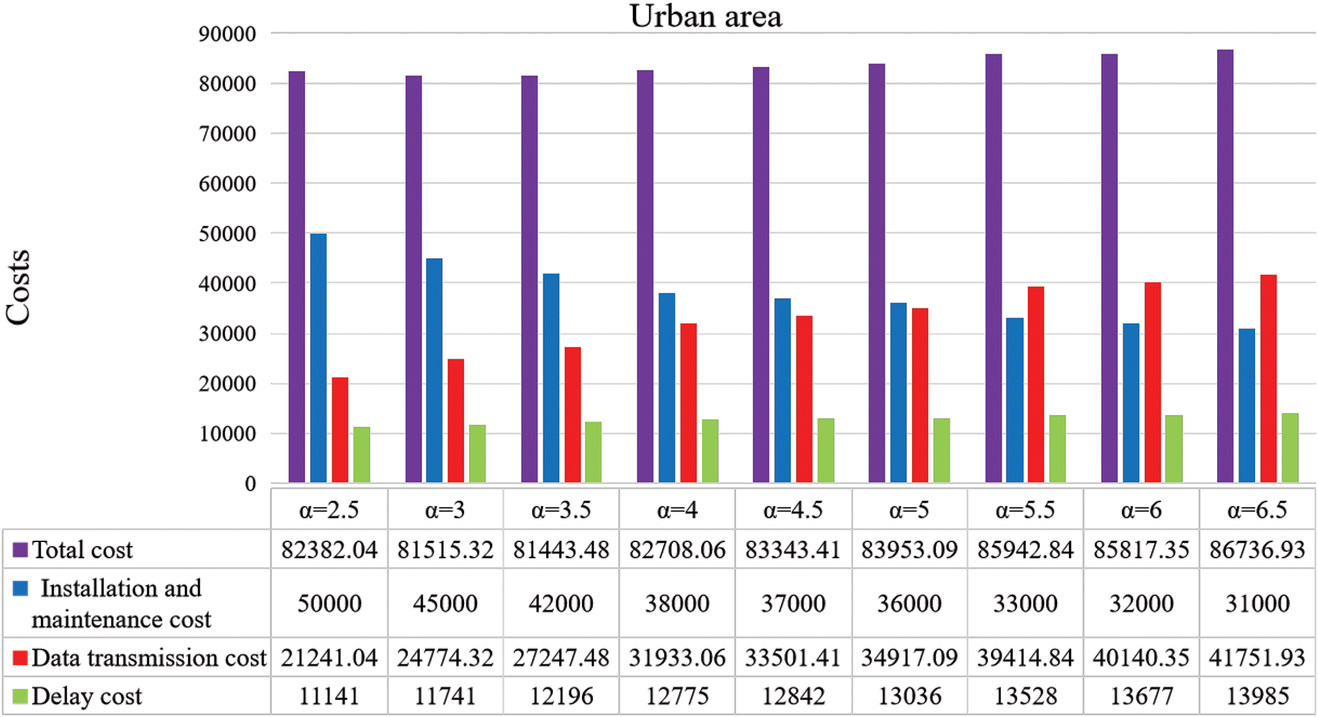
Fig. 7 illustrates the network costs associated with different $α$ values in urban areas. As $α$ decreases, the reference degree of SMs increases, prompting the APSSA algorithm to select more DAPs to form subnetworks wthin the wireless NAN network, which in turn, increases the installation and maintenance costs of DAPs. However, with increased DAPs, the average transmission distance and number of hops between SMs and DAPs decrease, thereby reducing data transmission and delay costs. In urban areas, the overall network cost is lowest when $α=3.5$ and highest when $α=6.5$ , where data transmission costs are considerably high.

images

Figure 7: Urban network costs

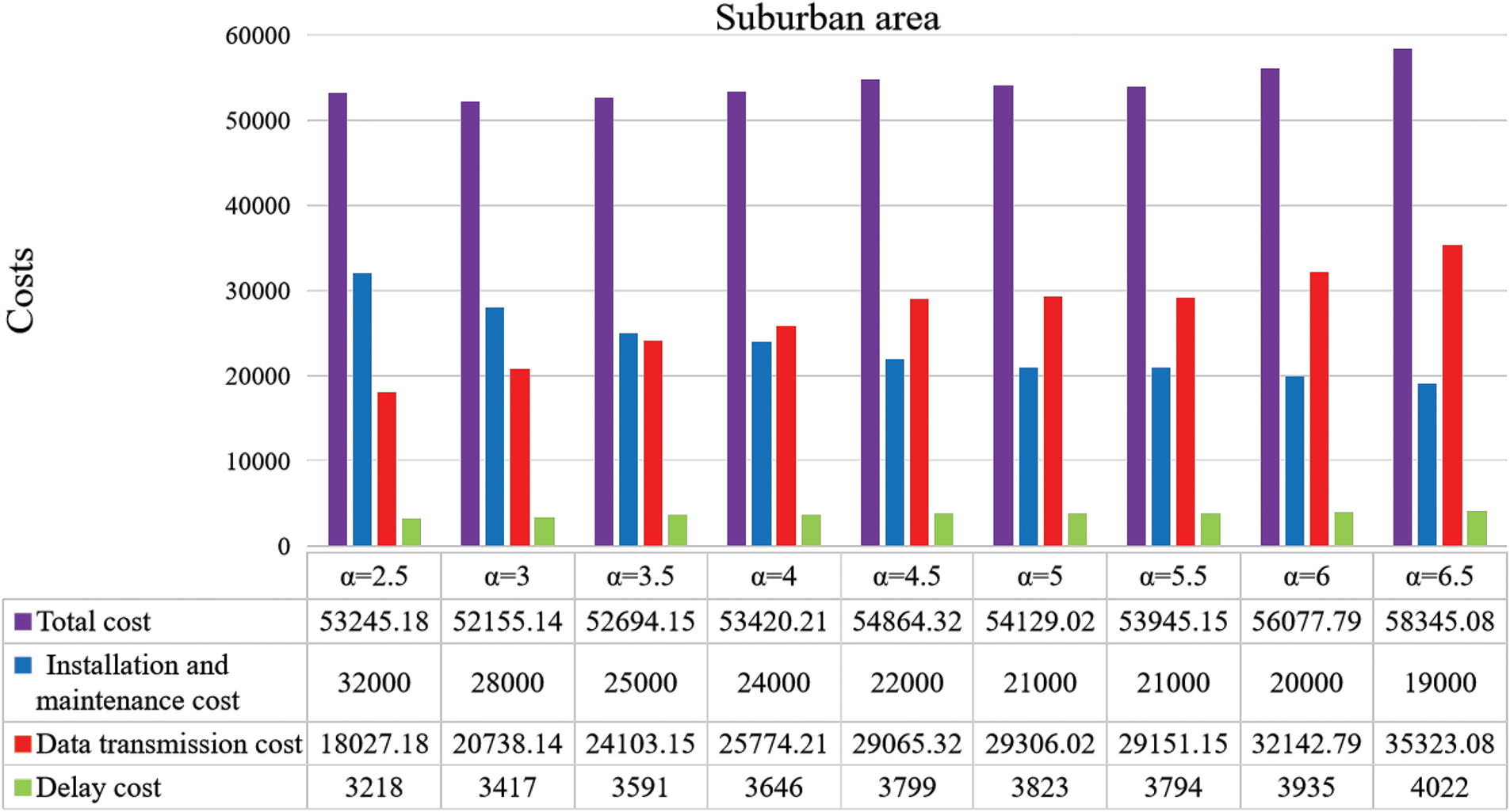
The trend of network costs in suburban areas with different $α$ values follows a pattern similar to that observed in urban scenarios, as shown in Fig. 8. As distance and hop count ecrease, data transmission and delay costs slo decline. In suburban areas, the overall network cost is lowest when $α=3$ , while it is highest at $α=6.5$ , where the number of installed DAPs is minimal. However, at $α=6.5$ , data transmission costs constitue a large proportion of the total network cost.

images

Figure 8: Suburban network costs

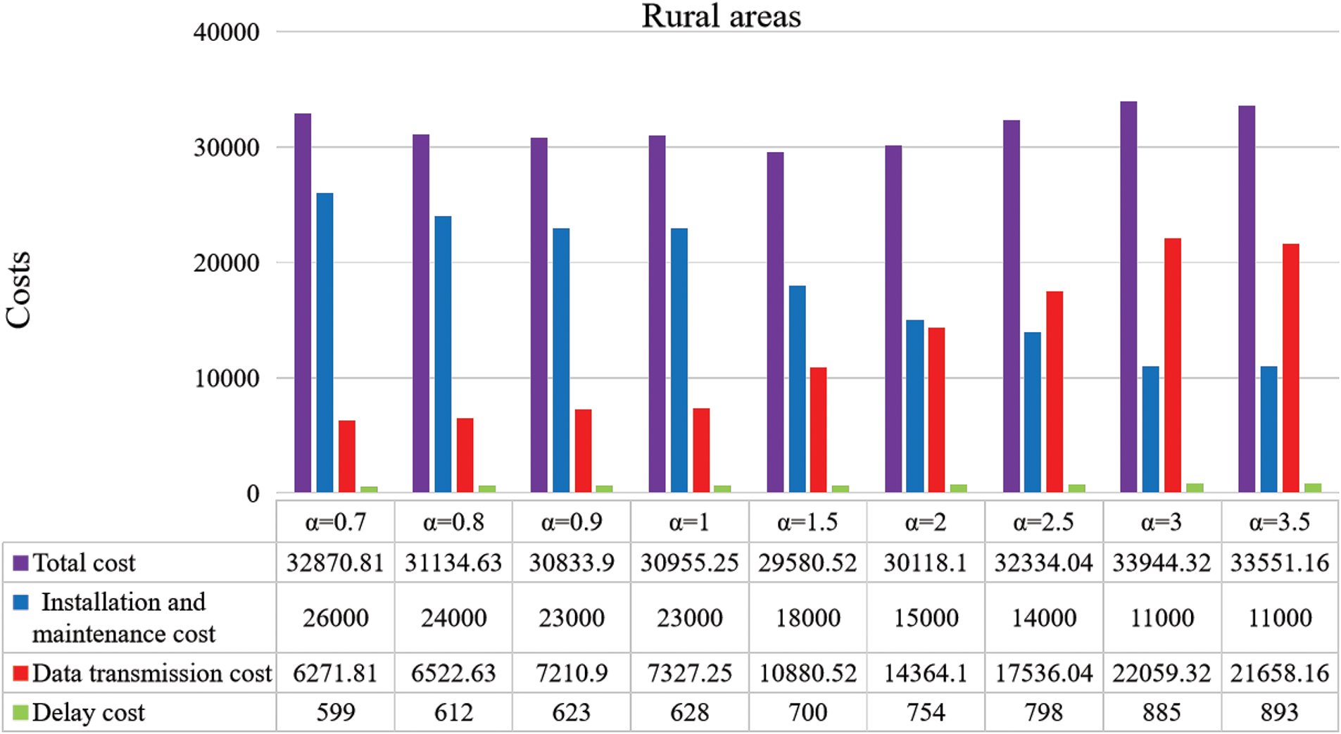
The network costs in rural areas for different values of $α$ are shown in Fig. 9. When $α=1.5$ , the transmission cost and delay costs are balanced against installation and maintenance costs, resulting in the lowest overall network cost. In constrast, at $α=3$ , the overall network cost is the highest. Compared with the urban and suburban areas, delay costs are notably higher in rural areas. This is due to the increased distribution density of SMs in rural areas, which shortens the transmission distance between them but increases the number of hops required for data transmission from SMs to DAPs.

images

Figure 9: Rural network costs

The number of SMs distributed is a key factor influencing $α$ values, as shown in Table 3. At lower $α$ values (e.g., $α=2$ and $α=3$ ), the number of DAPs increases with the number of SMs, although the growth rate may vary. In contrast, at higher $α$ values (e.g., $α=5$ and $α=6$ ), this growth trend is more moderate and sometimes remains constant. Overall, the number of DAPs is more sensitive to increases in SM count at lower $α$ values, but the total number of selected DAPs continue to rise as the number of SMs increases.

images

5.2 Analysis of the Distance Threshold $β$

To study the impact of the distance threshold $β$ on the APSSA algorithm, we similarly tested different values under the three regions. By testing different values of $β$ , we can better understand its impact on the optimized subnetwork and determine the best distance threshold setting. Notably, the values of the reference degree coefficient $α$ that we chose during our tests were all the lowest cost values, as mentioned before. It was executed 100 times in each scenario separately.

As shown in Fig. 10, in the urban area, when the value of $β$ was relatively small, the average transmission distance between SMs and DAPs in the whole network was small, whereas the load gap was large. As the value of $β$ increased, the average transmission distance gradually increased while the load gap gradually decreased. This was because, when the value of $β$ was small, the SM could allocate fewer DAPs and could only choose to communicate with the DAPs that were closer to it, which did not have a significant effect on reducing the load gap. As the distance threshold ( $β$ ) gradually increases, the number of DAPs that an SM can connect also increases, allowing SMs to join DAP subnets with lower loads and helping to balance the load among between different DAPs. However, since SMs initially communicate with nearby in the subnetwork formation process, switching to another DAP’s subnetwork leads to an increase in the average transmission distance.

images

Figure 10: Comparison of different $β$ -values—Urban: (a) Average transmission distance in urban; (b) Load gap in urban

In urban areas, when $β=1.2$ , the maximum average transmission distance is 185.98 m, and the minimum is 184.88 m. The load gap ranges from a maximum of 17.2 to a minimum of 13.15. Compared with $β=1.1$ and $β=1.3$ , $β=1.2$ effectively reduces the load gap among different DAPs, while keeping the average transmission distance minimal, achieving a more balanced.

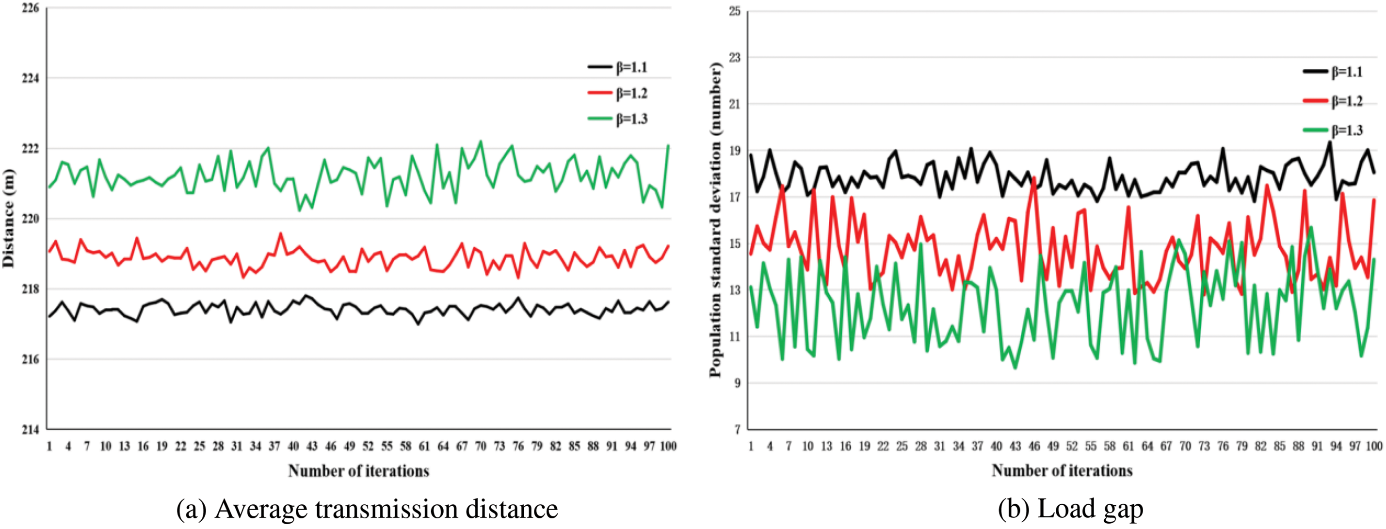
The effects of different $β$ values on the optimized subnetwork in suburban areas are shown in Fig. 11. As distance increases, the load gap decreases. When $β=1.2$ , the maximum average transmission distance is 219.57 m, and the minimum is 218.31 m. The load gap ranges from a minimum value of 17.8 to a minimum of 12.8.

images

Figure 11: Comparison of different $β$ -values—Suburban: (a) Average transmission distance in suburban; (b) Load gap in suburban

Similarly, the influence of different $β$ values on the optimal subnetwork in rural areas is shown in Fig. 12. The maximum load gap value is 3.90, while the minimum is 3.38. When $β=1.2$ , the increase in the average transmission distance of the wireless NAN network and the reduction in the load gap are relatively balanced, effectively optimizing both objectives. Therefore, $β=1.2$ is selected for subsequent experiments.

images

Figure 12: Comparison of different $β$ -values—Rural: (a) Average transmission distance in rural; (b) Load gap in rural

The transmission distance is a key factor influencing $β$ . The effect of transmission distance on the load gap under a fixed value of $β$ is shown in Table 4. Since the placement of SMs is random, no clear relationship exists between different numbers of SMs at the same transmission distance. However, as the transmission distance increases for a given number of SMs, the load gap between different DAPs gradually decreases, even if $β$ remains unchanged. This change occurs because a greater transmission distance allows SMs to connect to more distant DAPs, which, under the influence of $β$ , tend to be assigned to less-loaded DAPs, thereby reducing the load gap across different DAPs.

images

5.3 Comparison of Average Transmission Distance and Load Gap

In this subsection, the average transmission distance and DAP load gap of the proposed APSSA algorithm are compared with the K-medoids and $CDPAavg$ algorithms across three SM distribution density areas. Since K-medoids and $CDPAavg$ require a preset number of DAPs, the APSSA algorithm is first used to determine the number of DAPs for different wireless NAN networks. This number is then applied to K-medoids and $CDPAavg$ to ensure fair comparison. The value of $α$ in APSSA is set to the value that minimizes network cost in each region, with the distance threshold fixed at $β=1.2$ .

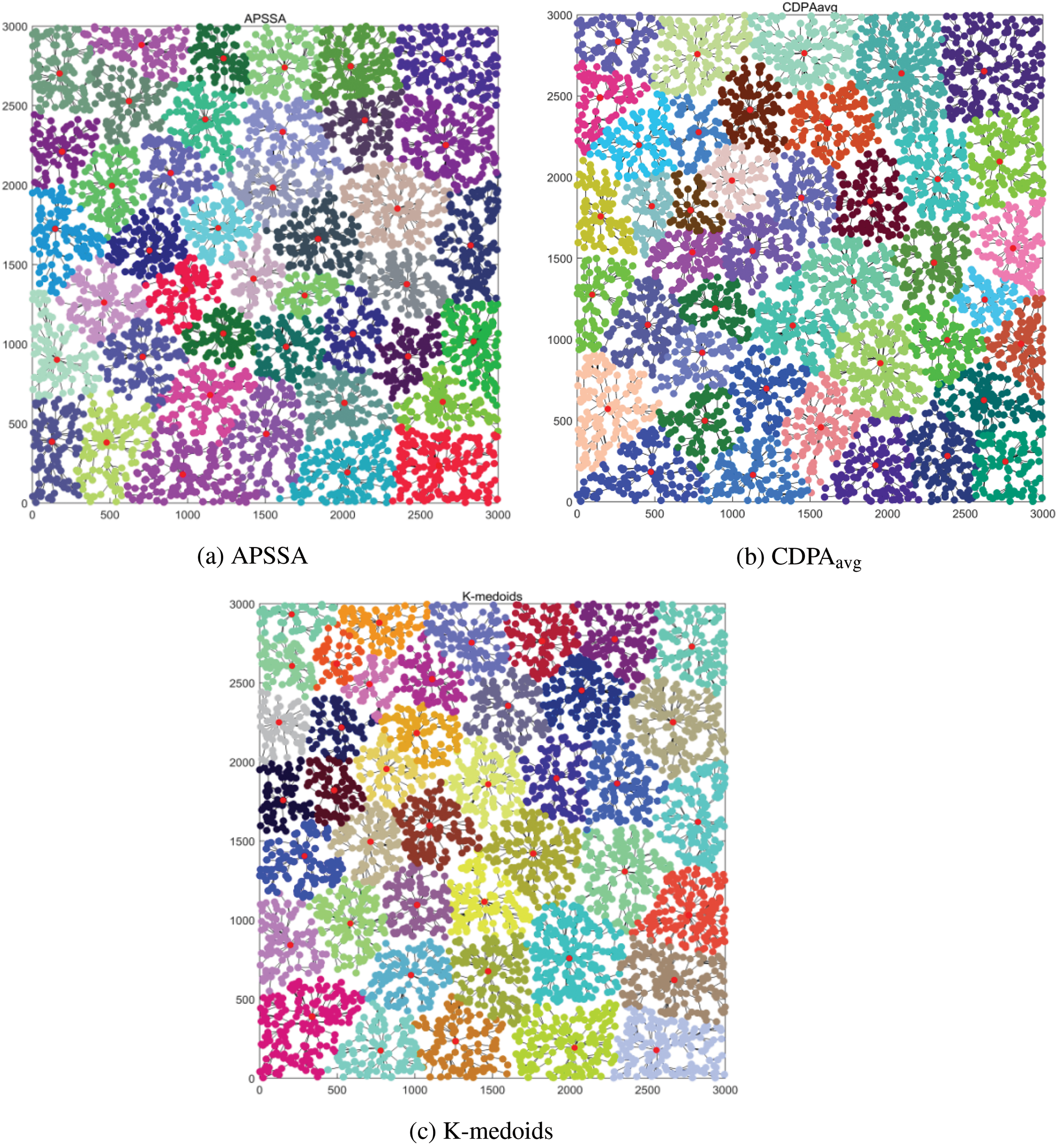
As shown in Fig. 13, the three DAP placement algorithms generate distinct DAP placements and subnetworks in urban areas. Fig. 13a shows the proposed APSSA algorithm, Fig. 13b illustrates the $CDPAavg$ algorithm, and Fig. 13c presents the K-medoids algorithm. In each figure, red dots indicate DAP placements, and different colors represent subnetworks formed by SMs within the NAN. Evidently, APSSA, K-medoids, and $CDPAavg$ yield different DAP placement results and subnetwork structures. Given the high SM distribution density in urban areas and the relatively short transmission distances between SMs, the average transmission distance between SMs and DAPs is lower in urban areas than in suburban and rural areas, whereas the SM coverage density per unit area of each DAP is the highest.

images

Figure 13: Demonstration of the three algorithmic realizations of DAP placement and the corresponding subnetwork—Urban: (a) Demonstration of the APSSA in urban; (b) Demonstration of the $CDPAavg$ in urban; (c) Demonstration of the K-medoids in urban

Fig. 14 shows the placements of DAPs selected by the three algorithms in the suburban area and the corresponding subnetworks formed by the different DAPs. In this scenario, 2000 SMs are distributed over the same area as in the urban area, but the SM density is lower. In addition, the suburban area has fewer DAPs than the urban area. Comparing Figs. 14 and 13, DAPs in suburban areas cover larger regions than those in urban areas, leading to an increase in the average transmission distance from SMs to DAPs and a decrease in the SM coverage density per DAP per unit area.

images

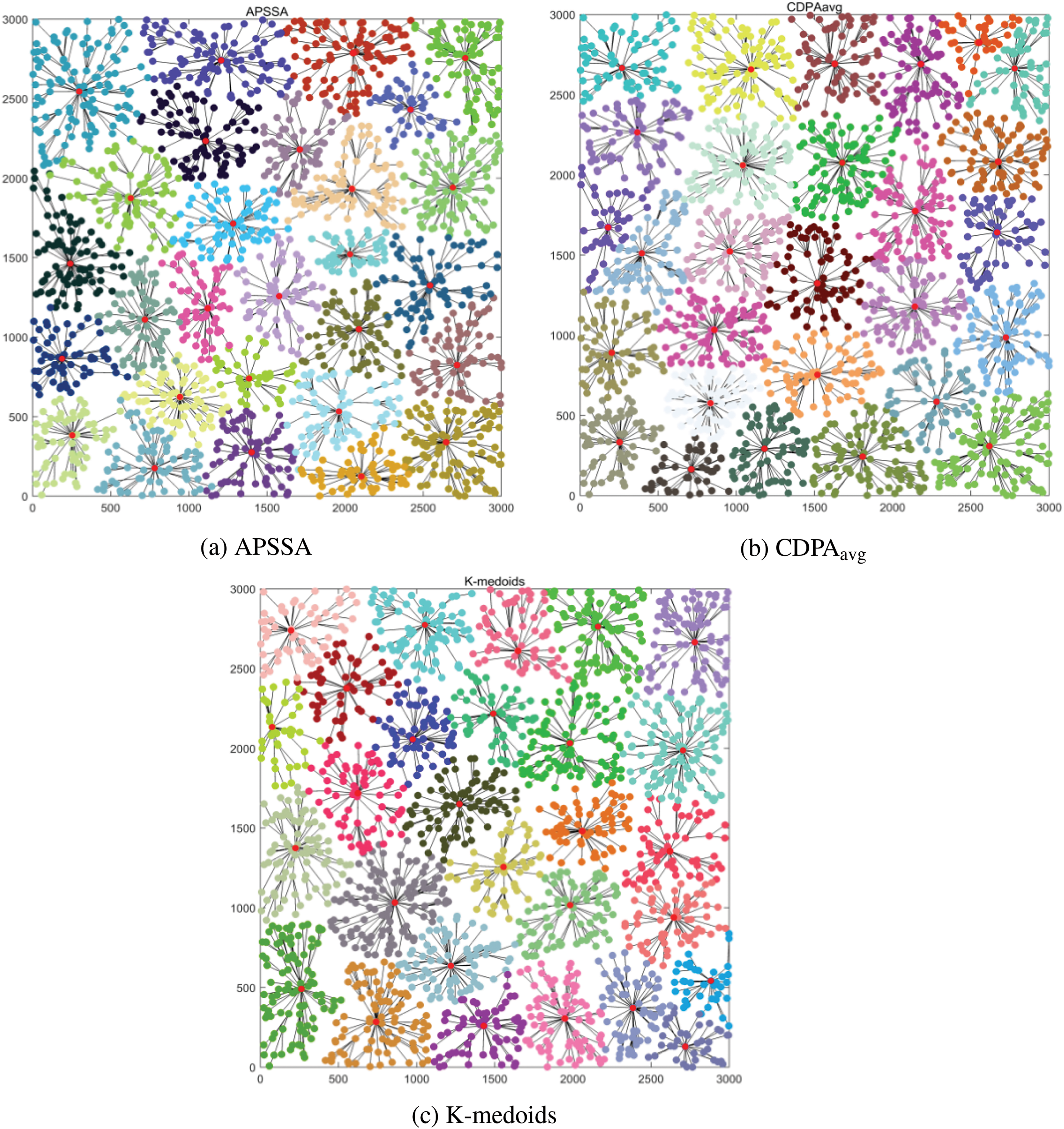
Figure 14: Demonstration of the three algorithmic realizations of DAP placement and the corresponding subnetwork—Suburban: (a) Demonstration of the APSSA in suburban; (b) Demonstration of the $CDPAavg$ in suburban; (c) Demonstration of the K-medoids in suburban

Fig. 15 presents the selected DAP placements and corresponding subnetworks for the three algorithms in rural areas. Compared with urban and suburban areas, SMs in rural areas are less densely distributed, the distance between SMs is larger, and the network contains communication links with longer transmission paths.

images

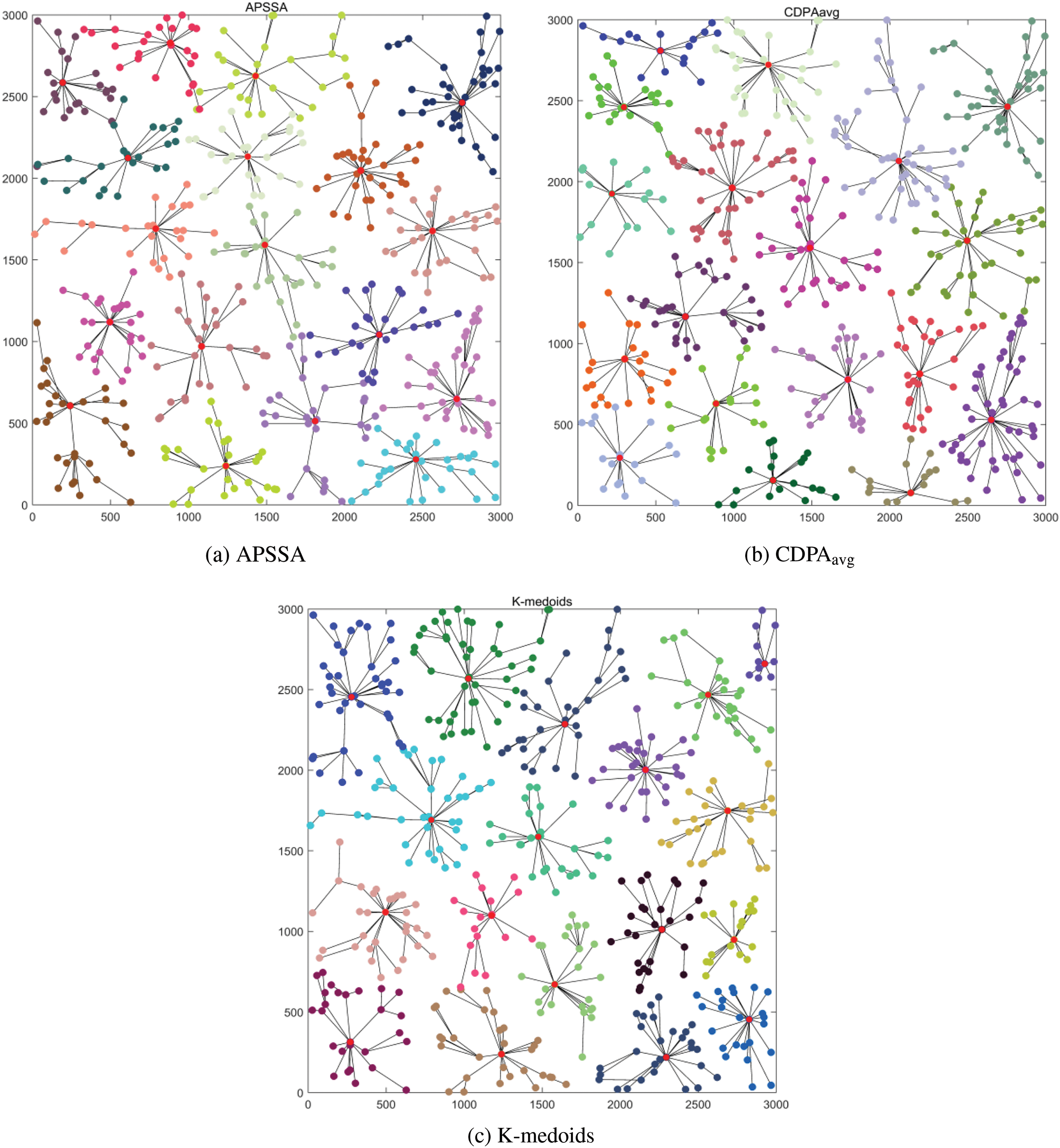
Figure 15: Demonstration of the three algorithmic realizations of DAP placement and the corresponding subnetwork—Rural: (a) Demonstration of the APSSA in ruarl; (b) Demonstration of the $CDPAavg$ in ruarl; (c) Demonstration of the K-medoids in ruarl

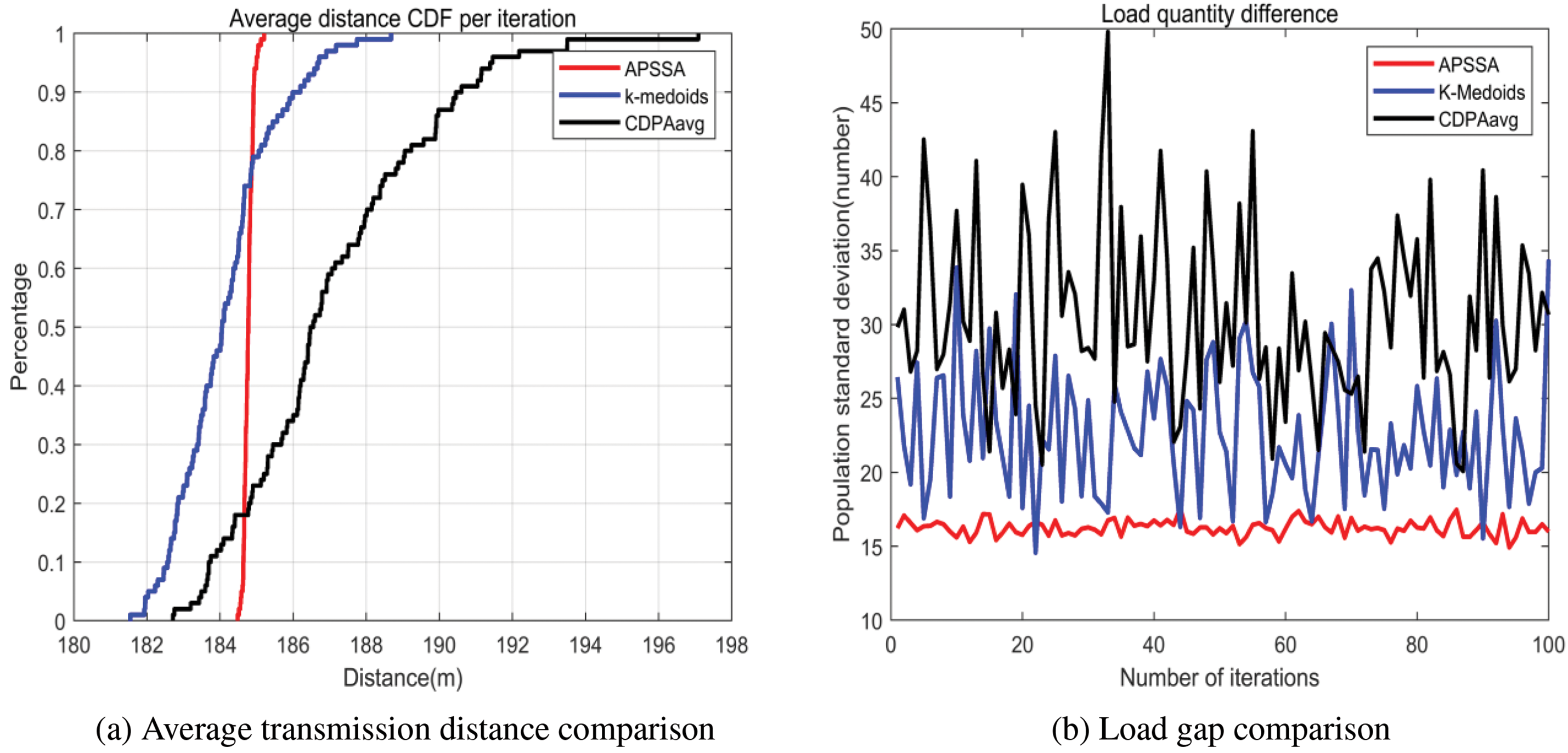
To reflect the real performance of the three algorithms, we executed each of them 100 times under each region and plotted the obtained results as cumulative distribution function (CDF) plots, as shown in Figs. 16–18. In this case, the reference degree coefficient $α$ in APSSA was chosen to be the value that minimized the cost of the network, and the distance threshold $β=1.2$ .

images

Figure 16: Comparison of average transmission distance and DAP load gap—Urban: (a) Average transmission distance comparison in urban; (b) Load gap comparison in urban

images

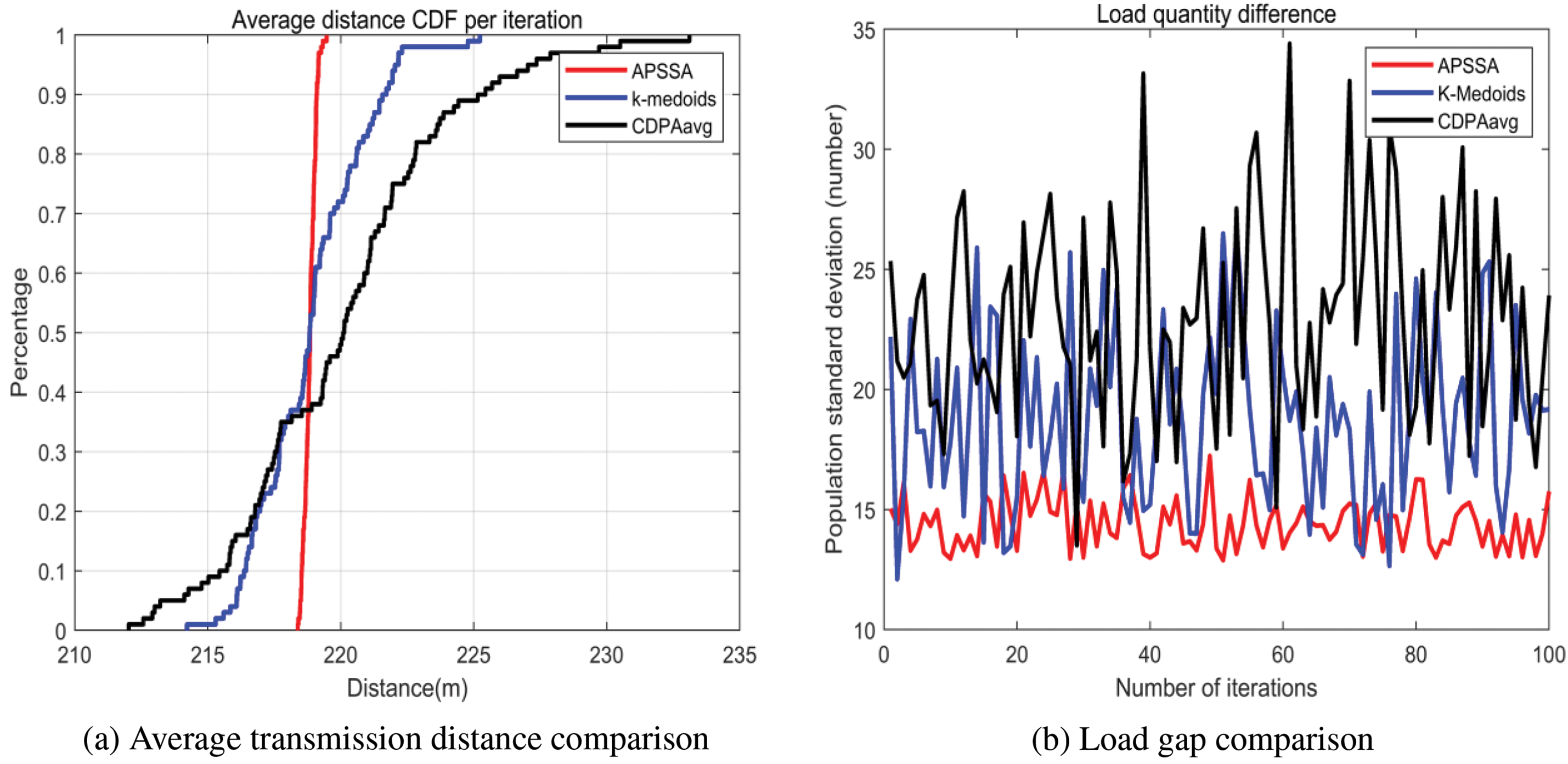
Figure 17: Comparison of average transmission distance and DAP load gap—Suburban: (a) Average transmission distance comparison in suburban; (b) Load gap comparison in suburban

images

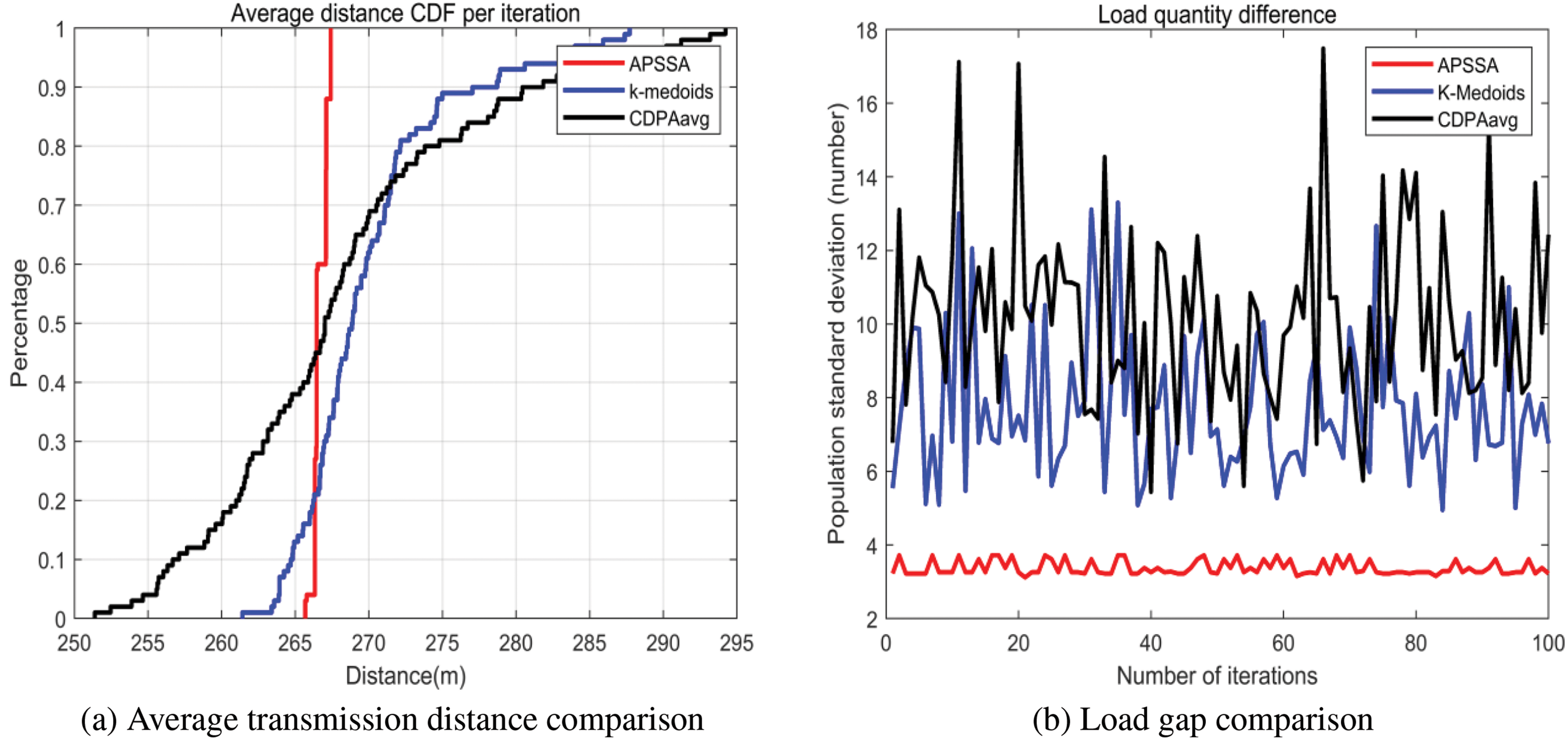
Figure 18: Comparison of average transmission distance and DAP load gap—Rural: (a) Average transmission distance comparison in rural; (b) Load gap comparison in rural

Fig. 16a depicts the plot of the CDF of the average transmission distance achieved by APSSA, K-medoids, and $CDPAavg$ under the urban area. Apparently, APSSA outperformed $CDPAavg$ in reducing the average transmission distance but did not have much advantage over K-medoids. Compared with K-medoids and $CDPAavg$ , APSSA had a narrower curve, which meant that the difference between the maximum and minimum values of the average distance produced by each run was smaller. Thus, APSSA was more stable compared with the other two algorithms. Fig. 16b illustrates the load gap generated by the three algorithms. The results demonstrate that the proposed APSSA algorithm maintains a load gap between 14.9 and 17.5, which demonstrates greater stability compared withthe $CDPAavg$ and K-medoids algorithms. In addition, the proposed APSSA algorithm achieves much smaller load gap than the other two algorithms.

The experimental results for the suburban area, shown in Fig. 17, indicate that the APSSA algorithm outperforms $CDPAavg$ and slightly outperforms K-medoids in terms of average transmission distance. In addition, APSSA demonstrates better stability, as the gap between its minimum and maximum average transmission distances is smaller than that of the other two algorithms. Regarding the load gap, APSSA achieves a range of 12.8–17.2, outperforming $CDPAavg$ and K-medoids. The average transmission distance for all three algorithms increases compared with the urban area, which is attributed to the lower SM distribution density in suburban areas, leading to greater distances between SM nodes and necessitating longer transmission distances to DAPs.

In rural areas, as shown in Fig. 18, APSSA outperforms $CDPAavg$ and K-medoids in terms of average transmission distance while also demonstrating greater stability. Regarding the load gap, APSSA achieves a maximum value of 3.72 and a minimum value of 3.11, thereby reducing the load imbalance across DAPs.

5.4 Analysis of the APSSA Algorithm

Time and space complexities are critical factors in algorithm design and selection. The time complexity directly influences the algorithm’s execution speed and determines its efficiency in handling large-scale data. In addition, space complexity pertains to the algorithm’s memory consumption, which affects its scalability and stability. In the smart grid DAP placement problem, selecting an optimal algorithm requires balancing these complexities based on problem-specific characteristics.

During NAN operation, the placement and number of installed DAPs installed considerably influence communication performance. First, DAPs’ placement directly influences the transmission distances between DAPs and SMs, thereby affecting the energy consumption and network transmission rates. Second, the number of installed DAPs determines the operational cost of NAN, which requires an optimal balance between cost efficiency and adequate network coverage. Finally, each DAP has a maximum load capacity that limits the number of SMs it can support. If a DAP exceeds its capacity, it may experience overload, leading to increased power transmission delays and hindering real-time monitoring and control of the SM information transmitted by the control center, thereby affects the normal operation of the power system. To comprehensively and efficiently address these challenges, we improved two well-performing DAP placement algorithms and developed the APSSA algorithm, optimizing placement strategies while ensuring improved network performance.

The time complexity of APSSA is $O(N3+pop×M×τ2)$ , where $N3$ represents core computations related to SM placement analysis for optimal DAP placement, while $pop×M×τ2$ accounts for the population-based load balancing iterations. By appropriately setting the population size M and iteration count $τ$ , APSSA ensures computational efficiency, even for large-scale SM deployments. Although $pop×M×τ2$ increases with the the number of SMs, its growth rate remains relatively controllable. Compared to other algorithms, APSSA achieves a superior balance between computational complexity and performance for large-scale data. The space complexity of APSSA is $O(N2+N×τ)$ , reflecting memory requirements for storing SM placements and computational results. While space complexity scales with the number of SMs, APSSA avoids excessive memory consumption, enabling stable operation in resource-constrained environments. These findings demonstrate that the APSSA algorithm exhibits good performance in both time and space complexity, making it well-suited for large-scale smart grids.

6 Conclusion and Future Directions

The number and location of DAPs affect the cost and quality of building NAN communication networks, and the DAP placement problem is more tightly constrained because of the different locations of SMs in different NANs. In this paper, we focused on the number and placement of DAPs in a NAN, aiming to minimize the average transmission distance between SMs and their DAPs while reducing the gap in the number of loads between different DAPs in the network. We described the objective functions of reducing the network cost, minimizing the average transmission distance, and reducing the gap in the number of loads in a NAN and proposed the APSSA algorithm based on the AP and SSA algorithms to solve the DAP placement problem. First, we improved the AP clustering algorithm, which enabled the APSSA algorithm to automatically select the appropriate number and location of DAPs based on the number and location of SMs to reduce the average distance. Second, we added an allocation mechanism in the SSA algorithm to optimize the subnetwork for balancing the loads of different DAPs and reducing the gap in the number of loads. In this paper, three different regions were selected to evaluate the APSSA algorithm and compare it with two other DAP placement algorithms. The experimental results demonstrated that our proposed APSSA algorithm can effectively shorten the average transmission distance, reduce the load gap, and outperform the other two DAP placement algorithms.

In the future, in addition to shortening the average transmission distance between DAPs and SMs and reducing the load gap, other objectives may include robustness and energy consumption. Actual DAP placement requires multiobjective optimization, which requires trade-offs between these objectives based on practical needs. When a DAP fails, it leads to a disconnection between the subnetwork where this DAP is located and the main network. This problem stimulates the research on the resilience and reliability of the AMI network for the failure of DAPs and SMs. Further experiments will validate APSSA in three large residential areas near Fujian University of Technology, each containing over ten buildings with 20–30 floors and multiple households per floor. These real-world scenarios will further assess APSSA’s effectiveness in large-scale deployments.

Acknowledgement: Thanks are extended to the editors and reviewers.

Funding Statement: This work was partially supported by the Fujian University of Technology under Grant GY-Z20016, GY-Z18183, and GY-Z19005, and partially supported by the National Science and Technology Council under Grant NSTC 113-2221-E-224-056-.

Author Contributions: Tien-Wen Sung: Conceptualization, Resources, Writing—Review & Editing, Supervision, Project Administration, Funding Acquisition. Wei Li: Conceptualization, Methodology, Software, Validation, Formal Analysis, Resources, Writing—Original Draft, Writing—Review & Editing. Yuzhen Chen: Software, Resources, Supervision. Chao-Yang Lee: Formal Analysis, Resources, Data Curation. Qingjun Fang: Formal Analysis, Data Curation, Supervision. All authors reviewed the results and approved the final version of the manuscript.

Availability of Data and Materials: Not applicable.

Ethics Approval: Not applicable.

Conflicts of Interest: The authors declare no conflicts of interest to report regarding the present study.

Nomenclature

DAP	Data Aggregation Point
SSA	Sparrow Search Algorithm
WAN	Wide Area Network
HAN	Home Area Network
NAN	Neighborhood Area Network
IoT	Internet of Things
SM	Smart Meter

References

1. Dileep G. A survey on smart grid technologies and applications. Renew Energy. 2019;146(1):2589–625. doi:10.1016/j.renene.2019.08.092. [Google Scholar] [CrossRef]

2. Omitaomu OA, Niu H. Artificial intelligence techniques in smart grid: a survey. Smart Cities. 2021;4(2):548–68. doi:10.3390/smartcities4020029. [Google Scholar] [CrossRef]

3. Sung TW, Xu Y, Hu X, Lee CY, Fang Q. Optimizing data aggregation point location with grid-based model for smart grids. J Intell Fuzzy Syst. 2022;42(4):3189–201. doi:10.3233/JIFS-210881. [Google Scholar] [CrossRef]

4. Ghosal A, Conti M. Key management systems for smart grid advanced metering infrastructure: a survey. IEEE Commun Surv Tutor. 2019;21(3):2831–48. doi:10.1109/COMST.2019.2907650. [Google Scholar] [CrossRef]

5. Wang Y, Chen Q, Hong T, Kang C. Review of smart meter data analytics: applications, methodologies, and challenges. IEEE Trans Smart Grid. 2018;10(3):3125–48. doi:10.1109/TSG.2018.2818167. [Google Scholar] [CrossRef]

6. Al-Salaymeh A, AlTwassi S, AlBeek R, Hassouneh K, Athamneh D, Alkiswani NE, et al. Smart meters rollout in Jordan: opportunities, business models, challenges, and recommendations. Int J Energy Econ Policy. 2022;12(4):394–408. doi:10.32479/ijeep.13008. [Google Scholar] [CrossRef]

7. Hsu HC, Zhuang SR, Huang YF. Cost-effective data aggregation method for smart grid. Electronics. 2021;10(23):2911. doi:10.3390/electronics10232911. [Google Scholar] [CrossRef]

8. Devidas AR, Ramesh MV. Cost optimal hybrid communication model for smart distribution grid. IEEE Trans Smart Grid. 2022;13(6):4931–42. doi:10.1109/TSG.2022.3185740. [Google Scholar] [CrossRef]

9. Renfov JRR, Pellenz ME, Santin AM. Insights on the resilience and capacity of AMI wireless networks. In: Proceedings of the IEEE Symposium on Computers and Communication (ISCC); Messina, Italy; 2016. p. 610–5. [Google Scholar]

10. Astudillo León JP, Duenas Santos CL, Mezher AM, Cárdenas Barrera J, Meng J, Castillo Guerra E. Exploring the potential, limitations, and future directions of wireless technologies in smart grid networks: a comparative analysis. Comput Netw. 2023;235(6):109956. doi:10.1016/j.comnet.2023.109956. [Google Scholar] [CrossRef]

11. Serper EZ, Altun-Kayhan A. Coverage and connectivity based lifetime maximization with topology update for WSN in smart grid applications. Comput Netw. 2022;209(2):108940. doi:10.1016/j.comnet.2022.108940. [Google Scholar] [CrossRef]

12. Aalamifar F, Shirazi GN, Noori MM. Cost-efficient data aggregation point placement for advanced metering infrastructure. In: Proceedings of the IEEE International Conference on Smart Grid Communications (SmartGridComm); Venice, Italy; 2014. p. 344–9. [Google Scholar]

13. Kong PY. Cost efficient data aggregation point placement with interdependent communication and power networks in smart grid. IEEE Trans Smart Grid. 2017;10(1):74–83. doi:10.1109/TSG.2017.2731988. [Google Scholar] [CrossRef]

14. Hassan A, Pu L, Luo Y. Data aggregation point placement in energy harvesting powered smart meter networks. In: Proceedings of the 11th International Conference on Modelling, Identification and Control (ICMIC2019); Tianjin, China; 2019. p. 831–41. [Google Scholar]

15. Li Y, Wang T, Wang S. Cost-efficient approximation algorithm for aggregation points planning in smart grid communications. Wireless Netw. 2020;26(1):521–30. doi:10.1007/s11276-019-02152-x. [Google Scholar] [CrossRef]

16. Gallardo JL, Ahmed MA, Jara N. Clustering algorithm-based network planning for advanced metering infrastructure in smart grid. IEEE Access. 2021;9:48992–9006. doi:10.1109/ACCESS.2021.3068752. [Google Scholar] [CrossRef]

17. Kong PY. Optimal configuration of interdependence between communication network and power grid. IEEE Trans Ind Informat. 2019;15(4):4504–065. doi:10.1109/TII.2019.2893132. [Google Scholar] [CrossRef]

18. Ghasempour A. Internet of things in smart grid: architecture, applications, services, technologies, and challenges. Inventions. 2019;4(1):22. doi:10.3390/inventions4010022. [Google Scholar] [CrossRef]

19. Meloni A, Pegoraro PA, Atzori L, Benign A, Sulis S. Cloud-based IoT solution for state estimation in smart grids: exploiting virtualization and edge-intelligence technologies. Comput Netw. 2018;130(15):156–65. doi:10.1016/j.comnet.2017.10.008. [Google Scholar] [CrossRef]

20. Sardar MAS, Hasi S, Sultan MN, Rabbi MDF. Intrusion detection in electric vehicles using machine learning with model explainability. J Inf Hiding Multim Signal Process. 2023;14(3):81–9. [Google Scholar]

21. Sung TW, Tsai PW, Gaber T, Lee CY. Artificial Intelligence of Things (AIoT) technologies and applications. Wirel Commun Mob Comput. 2021;2021:1–2. [Google Scholar]

22. Sung TW, Lee CY, Gaber T, Nassar H. Innovative artificial intelligence-based internet of things for smart cities and smart homes. Wirel Commun Mob Comput. 2023;2021:1–3. [Google Scholar]

23. Gallardo JL, Ahmed MA, Jara N. LoRa IoT-based architecture for advanced metering infrastructure in residential smart grid. IEEE Access. 2021;9:124295–312. doi:10.1109/ACCESS.2021.3110873. [Google Scholar] [CrossRef]

24. Khan A, Umar A, Munir A, Shirazi S, Khan M, Adnan M, et al. A QoS-aware machine learning-based framework for AMI applications in smart grids. Energies. 2021;14(23):8171. doi:10.3390/en14238171. [Google Scholar] [CrossRef]

25. Zhang Z, Liu M, Sun M, Deng R, Cheng P, Niyato D, et al. Vulnerability of machine learning approaches applied in IoT-based smart grid: a review. IEEE Internet Things J. 2024;11(11):18951–75. doi:10.1109/JIOT.2024.3349381. [Google Scholar] [CrossRef]

26. Zhang Z, Yang Z, Yau DKY, Tian Y, Ma J. Data security of machine learning applied in low-carbon smart grid: a formal model for the physics-constrained robustness. Appl Energy. 2023;347(1):121405. doi:10.1016/j.apenergy.2023.121405. [Google Scholar] [CrossRef]

27. Xu J, Lou H, Wang Z, Lu ZM. X-strip Y-band location clustering algorithm for network topology inference. J Inf Hiding Multim Signal Process. 2021;12(4):175–85. [Google Scholar]

28. Vrbsky L, da Silva MS, Cardoso DL, Frances CRL. Clustering techniques for data network planning in Smart Grids. In: Proceedings of the IEEE 14th International Conference on Networking, Sensing and Control (ICNSC); Calabria, Italy; 2017. p. 7–12. [Google Scholar]

29. Hassan A, Zhao Y, Pu L, Wang G, Sun H, Winter RM. Evaluation of clustering algorithms for DAP placement in wireless smart meter network. In: Proceedings of the International Conference on Modelling, Identification and Control (ICMIC); 2017; Kunming, China. p. 1085–90. doi:10.1109/ICMIC.2017.8321618. [Google Scholar] [CrossRef]

30. Molokomme DN, Chabalala CS, Bokoro PN. Enhancement of advanced metering infrastructure performance using unsupervised K-means clustering algorithm. Energies. 2021;14(9):2732. doi:10.3390/en14092732. [Google Scholar] [CrossRef]

31. Wang G, Zhao Y, Huang J, Winter RM. On the data aggregation point placement in smart meter networks. In: Proceedings of the International Conference on Computer Communication and Networks (ICCCN); Vancouver, BC, Canada; 2017. p. 1–6. doi:10.1109/ICCCN.2017.8038499. [Google Scholar] [CrossRef]

32. Wang G, Zhao Y, Ying Y, Huang J, Winter RM. Data aggregation point placement problem in neighborhood area networks of smart grid. Mob Netw Appl. 2018;23(4):696–708. doi:10.1007/s11036-018-1002-6. [Google Scholar] [CrossRef]

33. Bennett C, Wicker SB. Decreased time delay and security enhancement recommendations for AMI smart meter networks. In: Proceedings of the Innovative Smart Grid Technologies (ISGT); Gaithersburg, MD, USA; 2010. p. 1–6. [Google Scholar]

34. Lang A, Wang Y, Feng C, Stai E, Hug G. Data aggregation point placement for smart meters in the smart grid. IEEE Trans Smart Grid. 2021;13(1):541–54. doi:10.1109/TSG.2021.3119904. [Google Scholar] [CrossRef]

35. Luo C, Xing W, Cai S, Hu C. NuSC: an effective local search algorithm for solving the set covering problem. IEEE Trans Cybern. 2024;54(3):1403–16. doi:10.1109/TCYB.2022.3199147. [Google Scholar] [PubMed] [CrossRef]

36. Rolim G, Passos D, Albuquerque C, MOSKOU. A heuristic for data aggregator positioning in smart grids. IEEE Trans Smart Grid. 2017;9(6):6206–13. doi:10.1109/TSG.2017.2706962. [Google Scholar] [CrossRef]

Cite This Article

APA Style

Sung, T., Li, W., Lee, C., Chen, Y., Fang, Q. (2025). Data aggregation point placement and subnetwork optimization for smart grids. Computers, Materials & Continua, 83(1), 407–434. https://doi.org/10.32604/cmc.2025.061694

Vancouver Style

Sung T, Li W, Lee C, Chen Y, Fang Q. Data aggregation point placement and subnetwork optimization for smart grids. Comput Mater Contin. 2025;83(1):407–434. https://doi.org/10.32604/cmc.2025.061694

IEEE Style

T. Sung, W. Li, C. Lee, Y. Chen, and Q. Fang, “Data Aggregation Point Placement and Subnetwork Optimization for Smart Grids,” Comput. Mater. Contin., vol. 83, no. 1, pp. 407–434, 2025. https://doi.org/10.32604/cmc.2025.061694

BibTex EndNote RIS

Copyright © 2025 The Author(s). Published by Tech Science Press.
This work is licensed under a Creative Commons Attribution 4.0 International License , which permits unrestricted use, distribution, and reproduction in any medium, provided the original work is properly cited.

Table of Content

Data Aggregation Point Placement and Subnetwork Optimization for Smart Grids

Abstract

Keywords

References

Cite This Article

113

78

0

Related articles

Further Information

Guidelines

Follow Us

Join Us

Share Link