An Explainable Autoencoder-Based Feature Extraction Combined with CNN-LSTM-PSO Model for Improved Predictive Maintenance

1  Introduction

Predictive maintenance has become essential in today’s industrial landscape, providing a proactive approach to equipment upkeep that minimizes unexpected downtime and enhances operational efficiency. Traditionally, maintenance strategies have been categorized as reactive or preventive. Reactive maintenance addresses failures only after they occur, resulting in unplanned downtime and costly repairs. In contrast, preventive maintenance follows a fixed schedule, regardless of the equipment’s actual condition, often leading to unnecessary maintenance and resource waste. While both approaches are widely used, their limitations can be overcome through advanced, data-driven predictive maintenance strategies [1]. Predictive maintenance utilizes real-time data and advanced analytics to anticipate equipment failures, enabling timely interventions that prevent production disruptions. However, despite its potential, several challenges hinder its effectiveness and widespread adoption. One of the key challenges is the adaptability of predictive maintenance systems across diverse industrial environments. Machinery and operating conditions can differ significantly between industries, necessitating flexible and generalizable predictive models. Existing predictive maintenance methods often face challenges in maintaining accuracy and reliability across diverse equipment types and operational settings, resulting in inconsistent outcomes and diminished confidence in their predictions [2].

Over the years, various methods have been developed to overcome the challenges of predictive maintenance. Traditional approaches, such as reliability-centered maintenance and condition-based maintenance, rely on historical failure data and predefined thresholds to determine maintenance needs. Reliability-centered maintenance, for example, assumes a stable operating environment with well-defined failure modes, an assumption that often falls short in today’s dynamic and complex industrial systems. Similarly, condition-based maintenance continuously monitors specific indicators, such as vibration levels or temperature, but may fail to capture the full range of factors influencing equipment degradation. To address these limitations, machine learning and deep learning techniques have increasingly been adopted for predictive maintenance, offering more adaptive and data-driven solutions [3]. These methods have shown promise in modeling the complex relationships between operational data and equipment failures. For example, support vector machines, random forests, and artificial neural networks have been applied to predict failures based on sensor data [4]. Convolutional Neural Networks (CNNs) have been particularly effective in extracting features from raw data, while long short-term memory networks have been used to capture temporal dependencies in time-series data. Despite these advances, machine learning and deep learning methods are not without their challenges [5]. A key challenge in machine learning-based predictive maintenance is the quality and availability of data. Many industrial environments lack sufficient, high-quality data needed to train accurate models. Additionally, the available data is often heterogeneous, coming from various sensors and existing in multiple formats, which complicates data integration and preprocessing. Another key limitation is the lack of interpretability in many machine learning models, which are often perceived as black boxes, offering little transparency into the reasoning behind their predictions. This poses a significant concern in industries where understanding the rationale behind maintenance decisions is crucial, particularly in safety-critical applications. Furthermore, optimizing predictive models for different industrial scenarios remains difficult. Many existing models are designed for specific applications or datasets, reducing their effectiveness when applied to new environments. For example, a model trained on data from one type of machinery may struggle to predict failures in different equipment. This challenge of generalizability restricts the scalability of predictive maintenance solutions across industries, creating a major barrier to broader adoption.

Given these challenges, several critical research questions arise

a.   How can predictive maintenance models be made more adaptable and generalizable across various industrial environments?

b.   How can we improve the interpretability, explainability and transparency of these models to enhance their usability in safety-critical applications?

c.   How can we ensure that these models remain accurate and reliable even when data quality and availability vary?

To address these questions, this study proposes the following:

a.   A novel predictive maintenance framework integrates advanced deep learning techniques with optimization strategies for a robust, adaptable, and interpretable solution for predictive maintenance. This approach employs an Autoencoder for feature reduction, a CNN for feature extraction, and a Long Short-Term Memory (LSTM) network to capture temporal dependencies. To enhance interpretability, attention mechanisms are incorporated within the LSTM to highlight the most critical features that influence predictions, ensuring transparency and fairness in decision-making. Additionally, Particle Swarm Optimization (PSO) fine-tunes the model’s hyperparameters to ensure optimal performance across diverse datasets and industrial scenario.

b.   The proposed framework is validated using multiple datasets from diverse industrial environments, including sensor data from manufacturing equipment, power transmission systems, and other critical machinery.

c.   The performance of the proposed architecture is evaluated using various metrics, such as accuracy, precision, recall, F1-score, and training time, providing a comprehensive assessment of its effectiveness. The results demonstrate that the proposed approach outperforms traditional predictive maintenance methods and state-of-the-art machine learning models, achieving higher accuracy, better generalizability, and improved interpretability. Additionally, Receiver Operating Characteristic (ROC) curves have been deployed to validate the supremacy of the proposed model.

The rest of the manuscript is organized as follows. Section 3 highlights the Materials and Methods, wherein an extensive study of the existing methods has been performed under Related Works. This section also includes Methodology which incorporates the overall architecture, workflow, and algorithm contributing to the study. Section 4 presents the experimental analysis and results, this section, incorporates the datasets, evaluation metrics, results, and comparative analysis. Finally, Section 5 discusses the overall conclusion and future works.

2  Literature Review

Elkateb et al. [6] propose a predictive maintenance system using AdaBoost to classify various types of machine stops in real-time, specifically applied to knitting machines. The system utilizes data from IoT-enabled devices, including machine speeds and steps, which are pre-processed and classified into six categories of machine stops. With optimization through hyperparameter tuning and cross-validation, the model achieves a 92% accuracy rate, demonstrating its effectiveness in enhancing maintenance and productivity within the textile industry. However, the system’s effectiveness is demonstrated solely on knitting machines, and its applicability to other types of machinery remains unexplored, indicating a need for further research to assess its generalizability. In contrast, Arafat et al. [7] review the use of machine learning techniques in predictive maintenance for microgrid systems, emphasizing their role in improving failure prediction accuracy, fault detection, real-time diagnostics, and monitoring of microgrid components’ health and Remaining Useful Life (RUL). This study presents an overview of current machine learning methods, highlighting research gaps and proposing future frameworks to enhance predictive maintenance in microgrid systems. However, it remains primarily theoretical, emphasizing research gaps rather than providing practical case studies or implementation details that illustrate the real-world application of these methods in microgrid systems. Building on this, Jaenal et al. [8] introduce MachNet, a versatile deep learning architecture designed to address predictive maintenance challenges in Industry 4.0 environments. MachNet’s modular design allows it to integrate a range of sensors and other relevant data, such as asset age and material type, making it adaptable to diverse predictive maintenance scenarios. The study highlights that MachNet performs comparably or better than existing state-of-the-art methods in health state and RUL estimation tasks, demonstrating its general applicability and flexibility. However, the study lacks extensive discussion on MachNet’s computational requirements and scalability when applied to larger or more complex industrial systems, which is crucial for evaluating its broader applicability. Similarly, Abbas et al. [9] present a novel approach that integrates probabilistic modeling with deep reinforcement learning to enhance interpretability in safety-critical predictive maintenance. The framework employs input-output hidden Markov models to identify critical conditions, combined with behavioral cloning for baseline policy initialization, minimizing the need for extensive environmental interactions. When tested on turbofan engine predictive maintenance, the method surpasses existing approaches and enhances interpretability, making it adaptable to various predictive maintenance applications. However, its effectiveness is demonstrated through a case study on turbofan engines, which may limit its immediate applicability to other types of machinery or industries. Wang et al. [10] propose a comprehensive data-driven dynamic predictive maintenance strategy that integrates a deep learning ensemble method for system RUL prediction. This method combines a convolutional neural network with a bidirectional long short-term memory network to enhance RUL accuracy. The strategy also incorporates dynamic maintenance decisions, including order, stock, and maintenance actions, factoring in uncertain mission cycles. The experimental results using the National Aeronautics and Space Administration turbofan engine dataset show that the proposed approach outperforms traditional maintenance strategies. However, the study’s reliance on a specific dataset raises questions about the generalizability of this strategy to other industrial systems.

Dehghan Shoorkand et al. [11] address the challenge of integrating tactical production planning with predictive maintenance using a rolling horizon approach. They propose a hybrid deep learning method that combines CNN and long short-term memory networks to enhance the prediction accuracy of RUL for manufacturing systems. The method identifies optimal maintenance actions, which can be either perfect or imperfect, directly impacting the system’s operating state. This integrated approach is validated using a benchmarking dataset, showing a reduction in total production and maintenance costs compared to traditional methods. However, the study relies on a specific dataset that may not fully capture the complexities of diverse industrial settings or varying operational conditions, highlighting the need for further investigation into its broader applicability. Similarly, Kamariotis et al. [12] introduce a new metric for evaluating data-driven prognostic algorithms based on their impact on downstream predictive maintenance decisions, specifically component ordering and replacement planning. This metric, linked to decision settings and predictive maintenance policies, emphasizes optimizing maintenance planning to minimize long-run expected maintenance costs. The study employs this metric to optimize heuristic predictive maintenance policies and hyperparameters of prognostic algorithms, demonstrating its application through theoretical examples and simulations on turbofan engine degradation problems. While the proposed metric offers a performance assessment aligned with practical maintenance decision-making, its testing is primarily confined to simulations, which may not fully capture the real-world complexities and variances of actual industrial applications. Tseng et al. [13] introduce a novel deep learning module, Attention Long Short-Term Memory Projected, to improve RUL prediction. The Attention LSTM projected model integrates attention mechanisms with traditional LSTM networks to enhance the extraction of key features from long sequences. It also uses a time-window length method for better feature extraction. The results show that Attention LSTM projected outperforms traditional LSTM models and recent approaches while using fewer parameters, demonstrating improved efficiency in handling long-term dependencies. However, the study primarily compares Attention Long Short-Term Memory Projected with traditional and recent methods, with limited exploration of its performance in more complex or varied real-world scenarios, which may affect its broader applicability. In a related area, Khazaelpour et al. [14] propose a hybrid approach combining artificial intelligence and expert knowledge for time-series prediction in predictive maintenance. This approach integrates expert elicitation with a Full Consistently Method for optimization and Multi-Criteria Decision-Making to determine optimal weights. The study compares the performance of an artificial neural network with basic dynamic and static forecasts, finding that the Full Consistently Method for optimization and Multi-Criteria Decision-Making artificial neural network model significantly reduces root mean square error compared to traditional artificial neural network predictions. While this hybrid approach improves maintenance predictability and reduces overhaul costs, its applicability and performance in diverse industrial contexts beyond the specific case studied remain insufficiently explored. Jin et al. [15] provide a comprehensive review of how machine learning and digital twin technologies are integrated with additive manufacturing to enhance process optimization, defect detection, and sustainability. They examine various machine learning methods used in additive manufacturing, such as material analysis and process parameter optimization, and discuss the current state of digital twin-assisted additive manufacturing. The paper emphasizes the novel integration of big data, machine learning, and digital twins into a cohesive framework, offering valuable insights into future advancements and applications that could significantly improve additive manufacturing processes. However, the study provides a broad overview without offering in-depth case studies or empirical evidence to demonstrate the practical application and impact of the proposed framework in real-world additive manufacturing scenarios.

Martins et al. [16] propose a methodology for condition-based maintenance that enhances decision-making by predicting equipment states without requiring extensive data. The methodology integrates vibration sensor data with Deep Artificial Neural Networks for data imputation and uses a Hidden Markov Model for state classification, employing the Viterbi algorithm to determine equipment health states. The approach is validated through a case study on drying presses in the paper industry, demonstrating its robustness and potential generalizability to various types of equipment. However, while the methodology shows promising results, its effectiveness and generalizability are primarily demonstrated through a single case study, which may not fully account for variability across different industrial settings and equipment types, necessitating further exploration in broader contexts. Similarly, Chakroun et al. [17] present a predictive maintenance model utilizing machine learning and artificial intelligence to assess the health of critical machinery in a smart factory setting. Their focus is on two brass accessories assembly robots, specifically predicting the degradation of their power transmitters under severe conditions. The model, based on a Discrete Bayesian Filter, is compared to a Naïve Bayes Filter model, with Discrete Bayesian Filter showing superior predictive performance. The results, validated through testing, enable more informed maintenance scheduling. However, the study’s scope is limited to a specific type of machinery and environment, which may not fully capture the model’s effectiveness across different types of equipment or operational conditions, indicating the need for further validation in diverse industrial applications. Chapelin et al. [18] proposed a framework for drift detection and diagnosis in heterogeneous manufacturing processes, addressing key challenges in predictive maintenance. Their approach utilizes machine learning techniques to effectively detect and diagnose system drifts. The framework integrates novelty detection, ensemble learning, and continuous learning to improve scalability and adaptability across industrial environments. Validation using real-world metrics such as accuracy and precision demonstrates the framework’s robustness in practical settings. However, challenges persist in data availability, integration, and the generalizability of the approach to other industries. Iqbal et al. [19] proposed the Internet of Vehicle (IoV) TwinChain framework, which integrates Digital Twin, Machine Learning, and blockchain technologies for predictive maintenance of vehicles within the IoV. This framework aims to address the limitations of traditional reactive maintenance by proactively monitoring vehicle operating conditions to prevent failures and road breakdowns. Digital Twin provides real-time monitoring, while machine learning models, facilitate data-driven predictions. Blockchain is utilized to ensure data integrity and traceability across physical and twin environments. The authors implement a Proof of Concept using Microsoft Azure Digital Twin, Ethereum blockchain, and formal verification methods such as High-Level Petri Nets and Bounded Model-Checking, demonstrating the framework’s effectiveness in enhancing predictive maintenance and ensuring system reliability and accuracy in the IoV. Noura et al. [20] investigated fault detection and diagnosis in grid-connected photovoltaic systems using advanced machine learning tree-based algorithms. These systems integrate solar panels with the utility grid, providing significant benefits, such as low operating costs and reduced electricity bills. However, they remain vulnerable to downtimes and faults. The study applies Extra Trees in a two-phase framework, binary fault detection followed by multi-class fault diagnosis achieving accuracies of 99.5% and 98.7%, respectively. The research highlights the importance of oversampling for imbalanced datasets and incorporates explainable artificial intelligence to enhance model transparency. The findings support the framework’s scalability, simplicity, and effectiveness, demonstrating its potential for reliable fault detection in photovoltaic systems.

Based on the related works, predictive maintenance has emerged as a critical component in optimizing industrial operations, aiming to minimize downtime and improve efficiency. Traditional approaches have utilized various machine learning and deep learning techniques to forecast equipment failures and schedule maintenance. For instance, predictive models based on AdaBoost, Discrete Bayesian Filters, and hybrid neural networks architectures have shown promise in improving the accuracy of fault classification and RUL prediction. These methods often integrate complex models such as Autoencoder-CNN and LSTM for feature extraction, temporal modeling, and hyperparameter optimization. Despite these advancements, challenges persist, including the need for more adaptable and generalizable solutions that can handle diverse and evolving industrial environments. Existing methods often struggle with issues like limited interpretability, integration of expert knowledge, and the ability to adapt to varying sensor types and operational conditions. Moreover, many models are restricted to specific case studies or types of equipment, which may not generalize well across different contexts. To address these limitations, a novel predictive maintenance technique that integrates advanced deep learning architectures with optimization methods, aiming to enhance model performance and efficiency has been proposed. The proposed approach combines Autoencoder for dimensionality reduction, convolutional neural netroks for feature refinement, and LSTM for temporal dynamics, with PSO to fine-tune hyperparameters. This hybrid model seeks to overcome the constraints of traditional methods by offering greater flexibility, improved accuracy, and better adaptability to diverse industrial scenarios.

3  Methods

In this section, the architecture, workflow of the overall process and the algorithm used for conducting the study have been specified.

3.1 Architecture

The proposed architecture aims to tackle the challenges associated with accurately predicting the RUL of industrial systems. The model is designed to handle the complex relationships within the data by combining various advanced techniques, each playing a crucial role in the overall performance of the system. The components as discussed below, work together to provide a robust and efficient solution:

a.   Input Layer (Sensor Data)—The model begins by receiving raw sensor data, such as time-series information on temperature, pressure, and vibration, which reflect the system’s health. This high-dimensional data often contains spatial and temporal dependencies that must be captured effectively in the following layers.

b.   Encoder (Autoencoder)—The encoder compresses the input data into a lower-dimensional latent space, reducing noise and highlighting key features essential for predicting RUL. By minimizing reconstruction error, the encoder retains crucial data characteristics in the compressed form.

c.   Latent Space—The latent space stores the compressed data from the encoder, reducing computational complexity while preserving important information. It serves as a bridge, providing manageable and meaningful input for the subsequent CNN layer.

d.   Convolutional Neural Network—The network extracts spatial features from the latent space, detecting local patterns and hierarchical structures indicative of system degradation. It processes the input through convolutional layers, applying filters to capture both low-and high-level features essential for RUL prediction.

e.   Long Short-Term Memory with Attention—The network captures temporal dependencies, modeling how the system’s condition evolves over time. The integrated attention mechanism allows the model to focus on the most relevant time steps, enhancing its ability to understand and emphasize critical features for prediction. This improves the model’s interpretability, providing transparency in its decision-making process, which is crucial in safety-critical applications.

f.   Fully Connected Layer—The fully connected layer integrates the spatial and temporal features extracted by the CNN and LSTM, generating a unified representation. This layer is responsible for making the final predictions based on comprehensive data analysis.

g.   PSO—This optimization algorithm fine-tunes the model’s parameters to optimize performance, iteratively adjusting the network’s weights and biases to reduce prediction errors and improve generalization to new data.

h.   Output Layer—The output layer provides the predicted RUL, translating the optimized model output into a concrete prediction. This prediction informs maintenance decisions and quality checks, ensuring transparency through the attention mechanism and other interpretability techniques, which is especially important for industrial applications requiring clear, actionable insights.

Fig. 1 provides an overview of the architecture and components of the proposed model. Each component in the architecture plays a specific role, but it is their integration that makes the model truly powerful. The architecture processes data in stages: the encoder compresses input data, followed by CNN and LSTM layers that extract spatial and temporal features. The fully connected layer synthesizes these features, with PSO optimizing the model for improved predictions. The attention mechanism in the LSTM highlights critical time steps, enhancing prediction accuracy and model explainability. This hybrid architecture, combining autoencoders, CNN, LSTM, attention, and PSO, addresses RUL prediction challenges in complex systems and outperforms traditional methods, ensuring robust, generalizable results across various industrial applications.

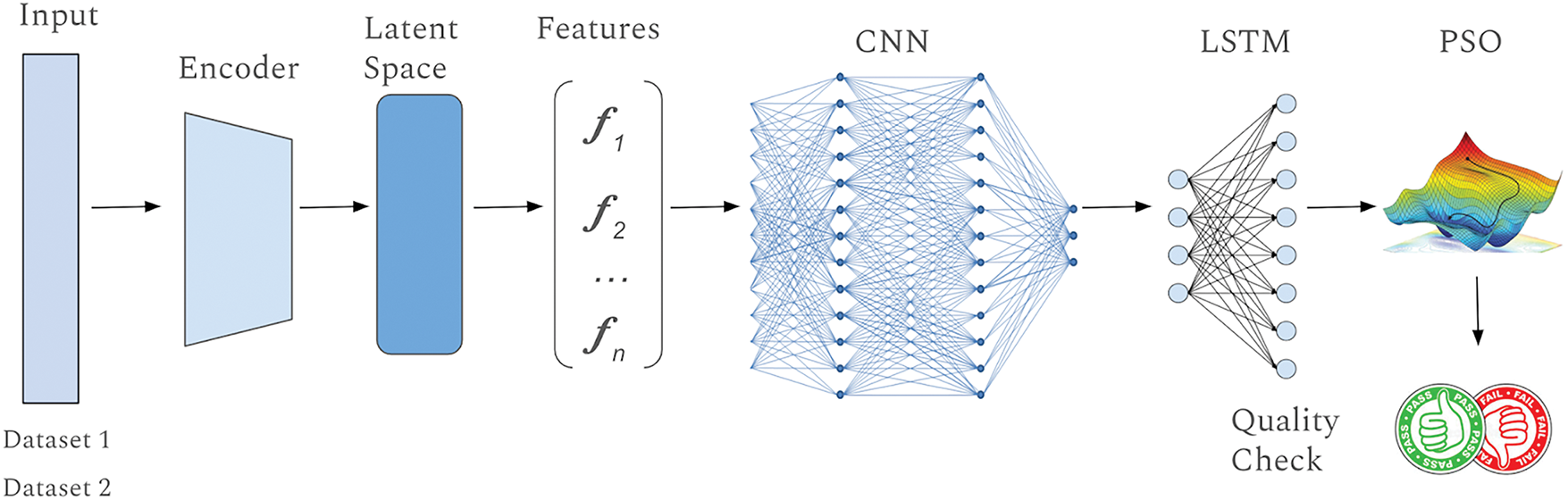
Figure 1: Architecture and overview of the proposed model

3.2 Workflow of the Overall Process

This section outlines the workflow of the machine learning pipeline used in this study, detailing how data is processed, transformed, and ultimately used within the proposed architecture. This workflow is essential for ensuring that the model accurately predicts the RUL of industrial systems. Additionally, this section also includes a few machine learning and deep learning algorithms that have been deployed to compare the performance of the proposed model.

a.   Data Acquisition is the first step in the workflow. In this stage, data is gathered from various industrial datasets. These datasets contain time-series information collected from sensors monitoring different components of machinery. The data typically includes parameters such as temperature, pressure, vibration, and other operational variables. These datasets are crucial as they provide the raw information necessary for building predictive models.

b.   Once the data is acquired, the next step is Data Preprocessing. This step involves cleaning the data to remove noise, outliers, or inconsistencies that could impact model performance. Missing values are handled through imputation techniques, while normalization or standardization is applied to ensure data comparability. To enhance explainability, certain key features are tagged during preprocessing with descriptors that clarify their impact on system health. For example, specific tags may denote ‘high-risk’ values, adding interpretability layers that highlight critical data points during model predictions. Downsampling or upsampling is also applied to address any class imbalance in the dataset.

c.   Following preprocessing, the data undergoes Feature Engineering. In this critical step, relevant features indicative of system degradation and RUL are extracted. This can include calculating the rate of change for specific parameters or aggregating data over time windows. Here, domain-specific knowledge is applied to label features with interpretable names or annotations, helping stakeholders understand the link between features and model output. The goal is to transform the raw data into informative features that enhance the model’s predictive capabilities.

d.   With the engineered features in place, the data is then split into Training and Testing Sets. In this study, the data has been split into 80% Training Data and 20% Test data. The training set is used to train the model, while the testing set is reserved for evaluating its performance.

e.   Model training begins with preprocessed data fed into the hybrid autoencoder-based CNN-LSTM network with PSO. The autoencoder compresses the data, the CNN extracts spatial features, and the LSTM captures temporal dependencies. PSO fine-tunes model parameters for optimal performance. Post-training, an explainability layer generates feature importance scores and highlights critical time steps, providing transparency into the factors influencing RUL predictions.

f.   To ensure the robustness and effectiveness of the proposed model, a comparative analysis has been conducted with several other well-known machine learning algorithms. These include K-Nearest Neighbors (KNN), Decision Tree (DT), Random Forest (RF), Gradient Boosting (GB), Support Vector Machine (SVM), Artificial Neural Network (ANN), CNN, LSTM, and CNN-LSTM with PSO. Each of these algorithms has been trained on the same data and evaluated using identical criteria to ensure a fair comparison. This step is crucial for highlighting the strengths of the proposed architecture and demonstrating its superiority in predicting RUL.

g.   After training, models are evaluated using metrics such as accuracy, precision, recall, F1-score, and training time. To make results more interpretable, model outputs include probability-based confidence scores, indicating the model’s certainty in each prediction. This layer of explainability allows users to trust the predictions, especially in safety-critical scenarios.

The choice of PSO over other optimization techniques is deliberate and based on both the computational and theoretical advantages PSO offers in several contexts.

a.   PSO is computationally simpler than many other bio-inspired algorithms. It relies on fewer hyperparameters to tune, such as the inertia weight and learning factors, which makes it well-suited for real-world applications where the objective is to balance performance and implementation complexity.

b.   PSO is known for its fast convergence in continuous optimization problems. This characteristic is particularly advantageous for scenarios where time and computational efficiency are critical, such as in predictive maintenance systems that need timely updates.

c.   The high-dimensional latent space produced by the Autoencoder requires an optimization algorithm capable of handling large parameter spaces efficiently. PSO’s mechanism of swarm intelligence effectively explores and exploits the search space, providing robust solutions even with a complex hybrid model.

d.   Unlike gradient-based methods, PSO does not rely on gradient information. This makes it an excellent choice for optimizing complex loss surfaces with non-differentiable or noisy regions, which are often encountered in AI architectures.

By incorporating advanced techniques such as autoencoders, CNN, LSTM, and PSO, the proposed architecture overcomes the limitations of traditional methods, offering more accurate and reliable RUL predictions. Furthermore, the integration of explainability techniques enhances transparency, allowing stakeholders to understand and trust the model’s predictions. Feature importance visualizations and model confidence indicators enable stakeholders to interpret RUL predictions, facilitating informed decision-making, particularly in preventive maintenance planning. The inclusion of multiple algorithms for comparison further underscores the effectiveness of the proposed approach, as it consistently outperforms these methods across various datasets and evaluation criteria. This comprehensive machine learning workflow not only enhances the accuracy of RUL predictions but also ensures that the model is robust, generalizable, and ready for practical deployment in predictive maintenance systems.

3.3 Algorithm

This section presents the detailed Autoencoder-Based Feature Extraction Combined with the CNN, LSTM, and PSO Model deployed for the study (Algorithm 1).

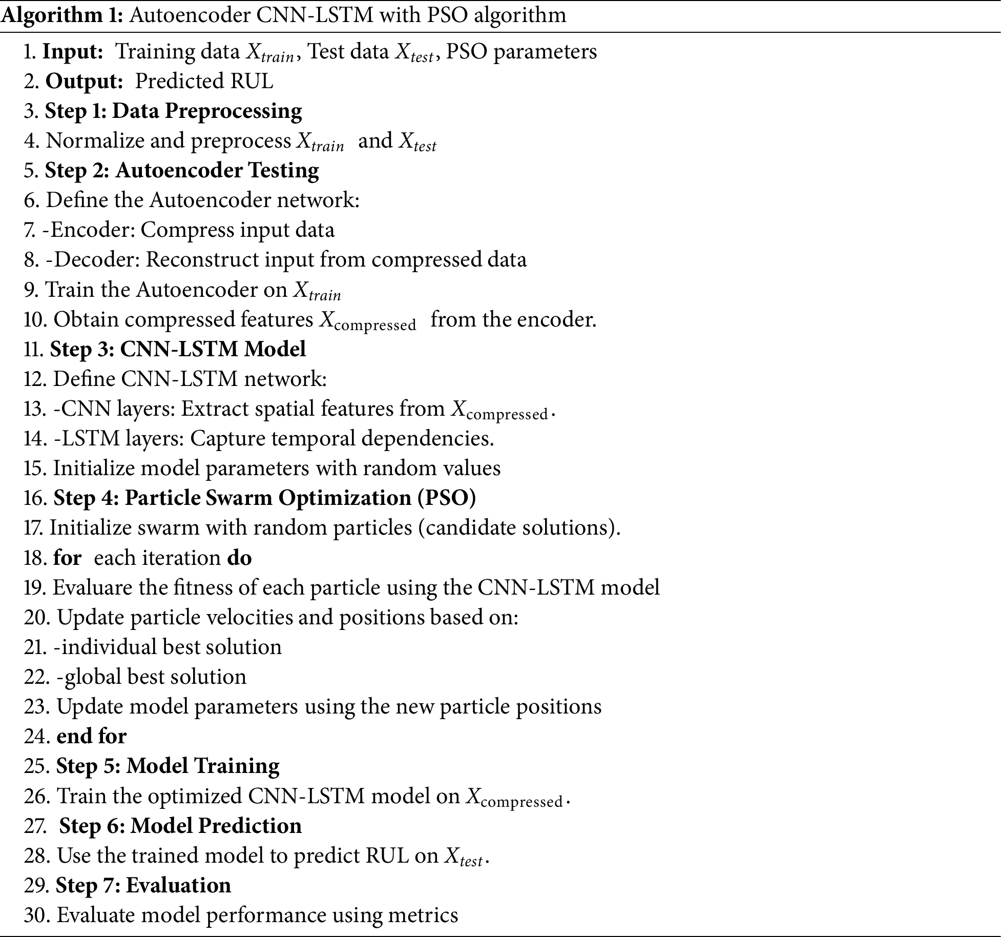
The algorithm starts with preprocessing, including normalization, handling missing data, and feature selection. The autoencoder, consisting of an Encoder and Decoder, compresses and reconstructs the input data. The encoder transforms the data into a compressed representation, which is then processed by the CNN, LSTM model. The CNN layers extract spatial features, while the LSTM layers capture temporal dependencies, combining both insights for RUL estimation. PSO fine-tunes the model parameters, ensuring optimal performance. This approach leverages the strengths of autoencoders, CNNs, LSTMs, and PSO to produce accurate predictions.

a.   A swarm of particles (potential solutions) is randomly initialized, such that each particle represents a set of model parameters.

b.   The fitness of each particle is evaluated using the CNN-LSTM model performance, typically by measuring a loss function such as Mean Squared Error (MSE) on a validation set.

c.   Each particle updates its velocity and position based on its own best-known position (individual best) and the best-known position of the entire swarm (global best).

d.   This process iterates until the particles converge to an optimal or near-optimal set of parameters, which are then used to train the CNN-LSTM model.

Once PSO has optimized the CNN-LSTM model’s parameters, the model is trained on the compressed features Xcompressed. The training involves backpropagation and gradient descent to minimize the loss function, allowing the model to learn the relationship between the input features and the RUL. After training, the optimized CNN-LSTM model is used to predict the RUL on the test data Xtest. The model’s performance is evaluated using several metrics, such as accuracy, precision, recall, etc.

3.4 Datasets

This study employs two different datasets to develop and validate the proposed predictive maintenance model, ensuring a comprehensive evaluation of the model’s effectiveness across varied industrial scenarios. The AI4I 2020 Predictive Maintenance Dataset focuses on machinery health and failure prediction, while the Parts Manufacturing-Industry Dataset emphasizes quality control in production. Both datasets were retrieved from Kaggle [21]. The first dataset, the AI4I 2020 Predictive Maintenance Dataset, is a synthetic dataset designed to closely mimic real-world conditions encountered in industrial settings. This dataset is particularly valuable for predictive maintenance tasks where access to real-world data can be limited due to privacy concerns or scarcity. The dataset comprises 10,000 instances, each representing a data point in the operational lifecycle of industrial equipment. It includes six critical features, such as air temperature, process temperature, rotational speed, torque, and tool wear, which are essential for predicting machine failure. The dataset also includes several types of failures, like tool wear failure, heat dissipation failure, power failure, overstrain failure, and random failures. Each failure mode is triggered by specific conditions, reflecting realistic scenarios where machinery might break down. For instance, tool wear failure occurs randomly between 200 to 240 min, while heat dissipation failure happens if the temperature difference falls below a certain threshold and rotational speed drops below a specified limit. This rich and diverse dataset enables the exploration of various predictive maintenance strategies, providing a robust foundation for testing our model. The second dataset, the Parts Manufacturing-Industry Dataset, focuses on defect detection in an industrial manufacturing context. This dataset contains details of 500 parts produced by each of the 20 operators within an industry over a specific period. Each operator has a different training background, introducing variability into the manufacturing process and making the dataset particularly challenging and realistic [22]. The dataset includes features such as the length, width, and height of the parts, and the operator responsible for their production. Unlike the first dataset, this one does not include explicit labels for defective or non-defective parts, which necessitates feature engineering. To classify the parts, we introduce a new feature, ‘status’ which determines whether a part is defective based on its dimensions. This determination is made by applying a function that compares each dimension (length, width, height) against acceptable ranges derived from boxplot statistics. If any of the dimensions fall outside these ranges, the part is labeled as ‘Defective’, otherwise, it is considered ‘Perfect.’ This feature engineering step adds another layer of complexity to the dataset, making it ideal for testing models designed to identify manufacturing defects and ensure product quality.

3.5 Evaluation Metrics

The following evaluation metrics have been used in the study (TP: True Positive, TN: True Negative, FP: False Positive, FN: False Negative):

a.   Accuracy: Accuracy measures the proportion of correct predictions made by the model out of all predictions. It is a general indicator of the model’s overall performance.

b.   Precision: Precision calculates the ratio of correctly predicted positive observations to the total predicted positives. It is useful in situations where the cost of false positives is high.

c.   Recall: Recall, also known as sensitivity, measures the ratio of correctly predicted positive observations to all observations in the actual class. It is crucial when the cost of false negatives is high.

d.   F1-score: The F1-score is the harmonic mean of precision and recall. It provides a single measure that balances both the concerns of precision and recall, especially in situations with class imbalance.

e.   Training Time: Training time refers to the total time taken to train the model. It is an important metric for assessing the computational efficiency of the model, especially for large datasets.

4  Methods

This section presents the results from the experimental analysis conducted within a Jupyter Lab environment. The study utilized TensorFlow for developing and training various neural network architectures, including CNN, LSTM networks, and their combined forms. For visualization and performance evaluation, Matplotlib was employed to generate insightful plots. Traditional machine learning models such as KNN, DT, RF, GB, and SVM were implemented using Scikit-learn, which facilitated data preprocessing and result assessment. This comprehensive approach enabled a detailed analysis of model performance, encompassing metrics such as accuracy, precision, recall, F1-scores, and training times.

4.1 Dataset 1

It is observed that most of most of the features do not follow the bell curve distribution in Fig. 2, and the data is skewed. The study deployed normalization techniques (Min-Max Normalization) to ensure that the data is well balanced.

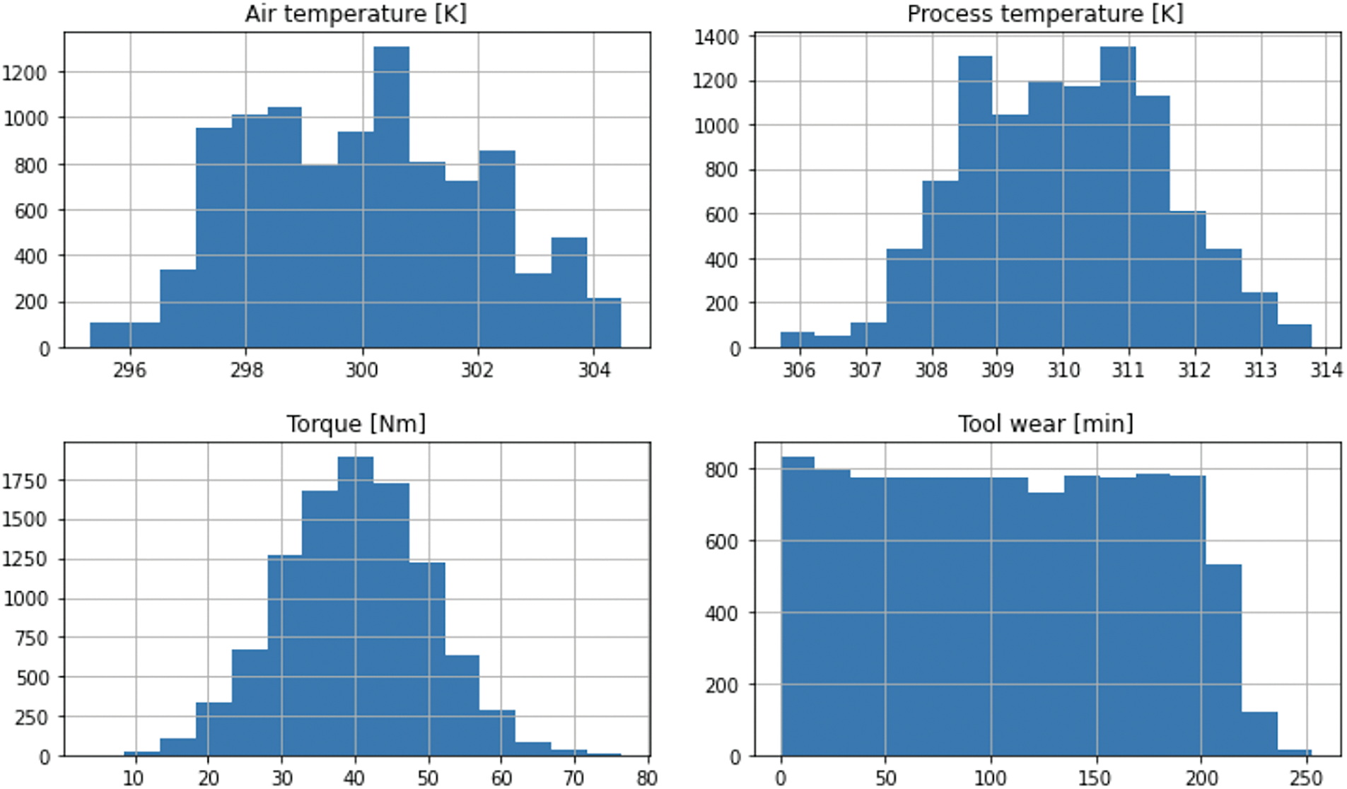
Figure 2: Distribution of features for Dataset 1

Fig. 3 illustrates the correlation matrix for Dataset 1. It shows that the correlations among the features are balanced, with no features exhibiting strong positive or negative relationships. As a result, no features were removed, and the algorithms were applied to the complete dataset.

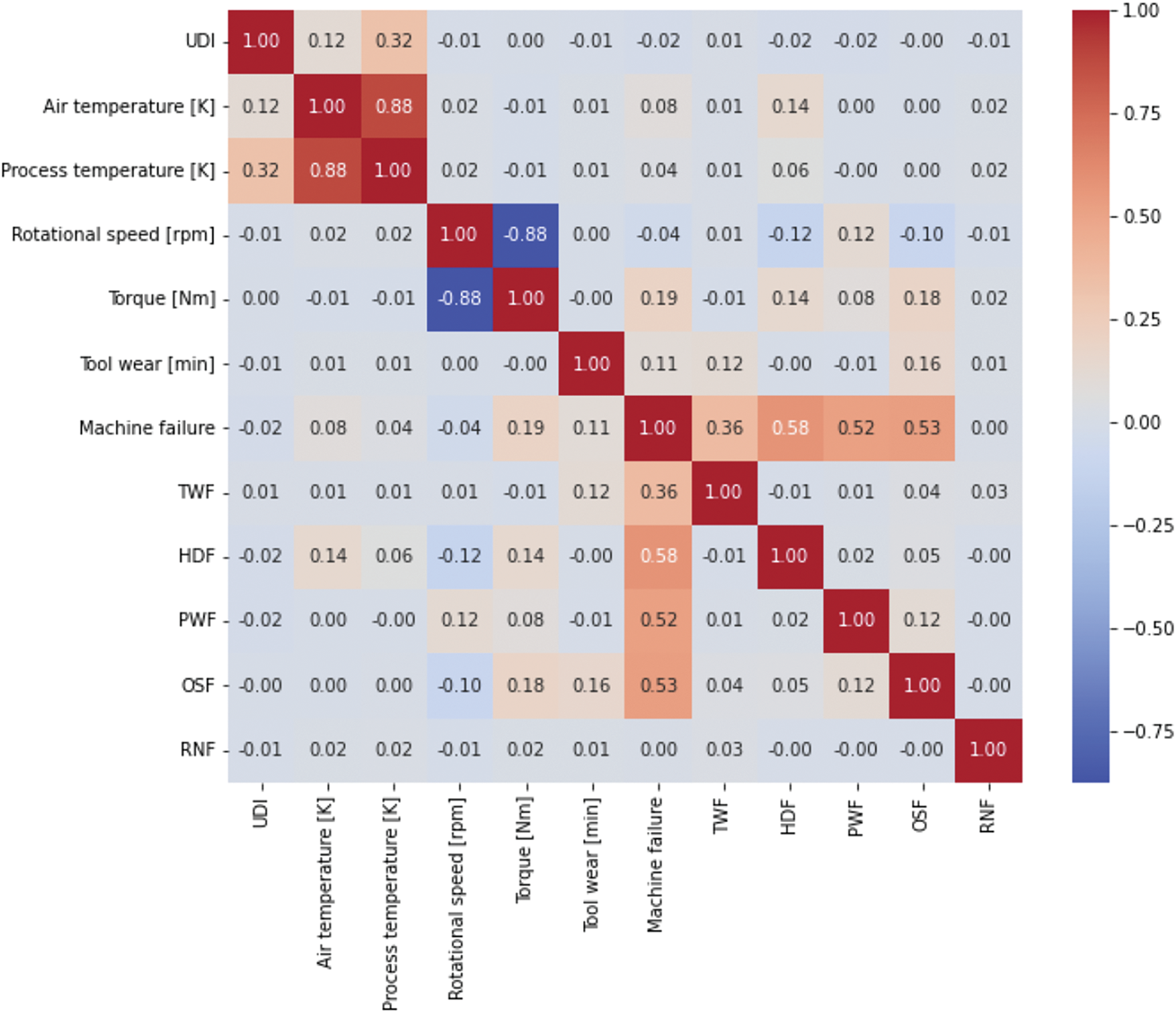
Figure 3: Correlation matrix for Dataset 1

Table 1 depicts the performance evaluation of the algorithms deployed.

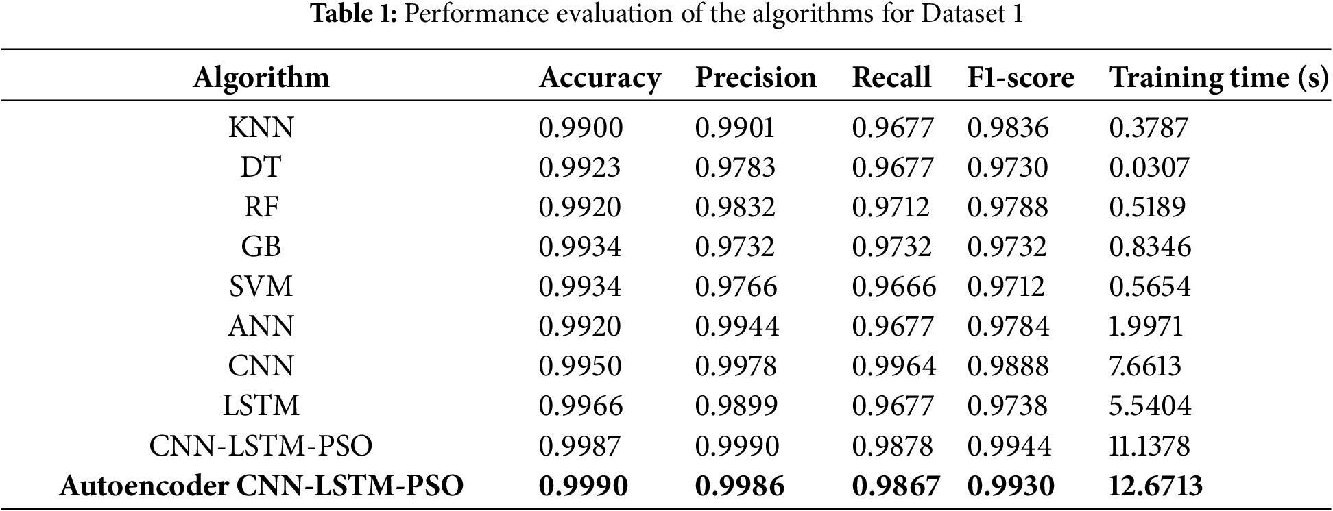
Based on the experimental analysis, it is observed that the KNN algorithm achieved high accuracy and precision with relatively low training time, indicating its efficiency in handling the dataset. DT and RF also performed well, with DT showing the quickest training time (0.0307 s), likely due to its simpler structure compared to more complex models. GB and SVM offered robust performance with slightly longer training times, but they were still within reasonable limits given their accuracy and precision. ANN showed good performance (0.9920) but with a significantly higher training time (1.9971 s), reflecting the complexity of training deep networks. CNN and LSTM provided even higher accuracy and precision, with CNN achieving the best F1-score (0.9888). However, both models had longer training times, indicating the computational demands of deep learning approaches. The CNN-LSTM-PSO model, combining both CNN and LSTM with PSO, exhibited exceptional accuracy (0.9987) and precision (0.9990) but at the cost of an even longer training time. Finally, the Autoencoder-CNN-LSTM-PSO model demonstrated the highest performance metrics and was the most accurate (0.9990), though it also had the highest training time (12.6713 s), underscoring the trade-off between performance and computational cost in complex models (Fig. 4).

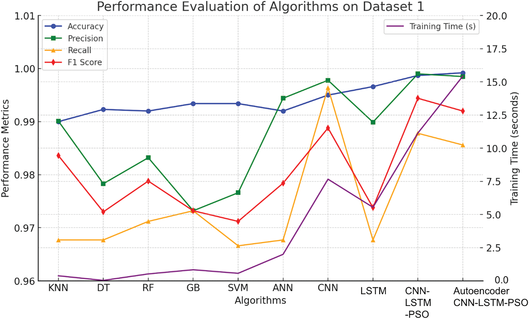
Figure 4: Performance evaluation of algorithms for Dataset 1

For the CNN-LSTM model optimized with PSO, the network has been trained with 64 filters in the convolutional layers, which strikes a balance between complexity and computational efficiency. For the kernel size, a value of 5 is selected to capture meaningful spatial patterns in the data. The LSTM units are set to 100, providing sufficient capacity to model temporal dependencies without being overly complex. The time steps are chosen to be 20, reflecting a moderate sequence length suitable for capturing relevant temporal information. After preprocessing, the number of features is set to 30, which balances detail and model complexity. In this setup, the PSO algorithm uses a swarm size of 10 and performs 5 iterations, allowing the exploration of the parameter space while keeping the computation manageable.

For the Autoencoder-CNN-LSTM-PSO model, the hyperparameters are set to optimize the model’s performance across its components. The autoencoder consists of two hidden layers in the encoder with 128 and 64 units, respectively, using Rectified Linear Unit (ReLU) activation, and a latent dimension of 32 units. The autoencoder is trained with an Adam optimizer, MSE loss function, and a batch size of 64, and 50 epochs. For the CNN component, the model features two convolutional layers with 64 and 128 filters, both using a kernel size of 3, ReLU activation, and a max pooling size of 2. The CNN uses a dropout rate of 0.5 and is trained with a batch size of 64 over 30 epochs. The LSTM layer has 100 units with a dropout rate of 0.3 and is also trained with a batch size of 64 and 30 epochs. PSO is employed with 20 particles, 10 iterations, an inertia weight of 0.7, and both cognitive and social parameters set at 1.5. The learning rate for both CNN and LSTM components is set to 0.001. Regularization includes L2 regularization with a weight of 0.01 applied to CNN layers and a dropout rate of 0.3 in LSTM layers to prevent overfitting.

Fig. 5 depicts the ROC curve, which is a crucial tool for evaluating the performance of classification models, especially in cases where the datasets are imbalanced. It provides a visual representation of the trade-off between sensitivity True Positive Rate (TPR) and specificity False Positive Rate (FPR) across different threshold settings. For Dataset 1, the ROC curves highlight the performance of various algorithms, with the Autoencoder CNN-LSTM-PSO model standing out due to its superior Area Under the Curve (AUC) value of approximately 0.99. This indicates that the model has an exceptional ability to distinguish between positive and negative classes. The gradual increase in the TPR while maintaining a low FPR for the Autoencoder CNN-LSTM-PSO model underscores its robustness and accuracy in predictive maintenance tasks. Other models, such as the standard CNN-LSTM-PSO, also performed well, but the Autoencoder enhancement provided a noticeable improvement in classification performance.

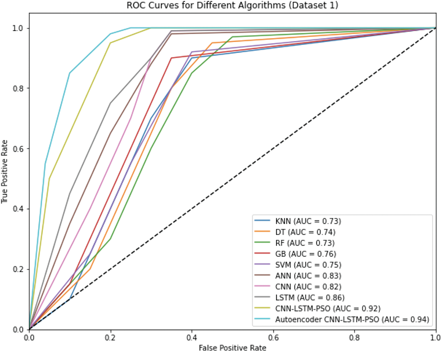
Figure 5: Performance evaluation of algorithms for Dataset 1 using ROC curves

The experimental results on Dataset 1 highlight the explainability embedded within the Autoencoder-CNN-LSTM-PSO model, especially its strong ability to identify key patterns relevant to predictive maintenance. The model’s high AUC score of around 0.99 (Fig. 5) demonstrates a strong capacity to separate positive from negative outcomes across different thresholds, which is valuable for prioritizing machinery based on their risk levels. This distinction supports users in understanding which components may require maintenance soonest, helping them address potential issues proactively. Explainability in this model operates on several levels.

a.   The autoencoder effectively reduces data dimensionality by isolating essential features such as temperature, pressure, and vibration patterns thus focusing on critical factors influencing RUL while filtering out irrelevant information. By simplifying input features to their most informative core, the autoencoder enhances interpretability, as users gain clearer insights into the factors that weigh most heavily in each prediction.

b.   The CNN layers, equipped with a kernel size of 3 and 64 filters, focus on capturing localized data trends, which helps detect sudden changes or anomalies that often indicate early stages of mechanical issues. This localized detection adds a layer of interpretability by showing which specific readings such as a spike in vibration or a temperature anomaly are contributing to the RUL forecast.

c.   Temporal explainability comes from the LSTM layer’s 100 units, which track system conditions over time, helping to model how wear and usage patterns affect predictions. This time-sensitive approach is useful for understanding the role of historical data, showing users how past conditions influence future RUL, which is essential in maintenance planning.

d.   PSO further fine-tunes the model’s parameters, ensuring that its decisions are grounded in a balance between predictive accuracy and computational efficiency.

e.   Finally, the ROC curve offers a visual perspective on the model’s performance, illustrating its sensitivity and specificity across various thresholds. The Autoencoder-CNN-LSTM-PSO model’s ability to maintain a high TPR with minimal FPR underscores its precision in identifying high-risk cases, which makes the model’s outputs easier to trust and act upon in practical settings.

Upon analyzing the experimental results, it is observed that while the Autoencoder-CNN-LSTM-PSO model achieves the highest performance in terms of accuracy (0.9992), this comes at the cost of significantly higher computational time (15.4321 s) compared to simpler models such as DT (0.9923, 0.0307 s) and LSTM (0.9966, 5.5404 s). The improvement in accuracy is relatively marginal (<0.5%), which raises the critical question of whether the performance gain justifies the increased computational cost. In safety-critical applications, where accurate predictions directly impact operational efficiency and resource allocation, even small performance improvements are deemed valuable. However, for environments requiring real-time predictions, models like CNN and LSTM, which offer high accuracy with lower computational time (7.6613 s and 5.5404 s, respectively), may be more practical.

4.2 Dataset 2

This dataset seems to be more balanced compared to the other dataset as seen in Fig. 6, however a few parameters show a skewed distribution. The study deployed normalization techniques (Min-Max Normalization) to ensure that the data is well balanced.

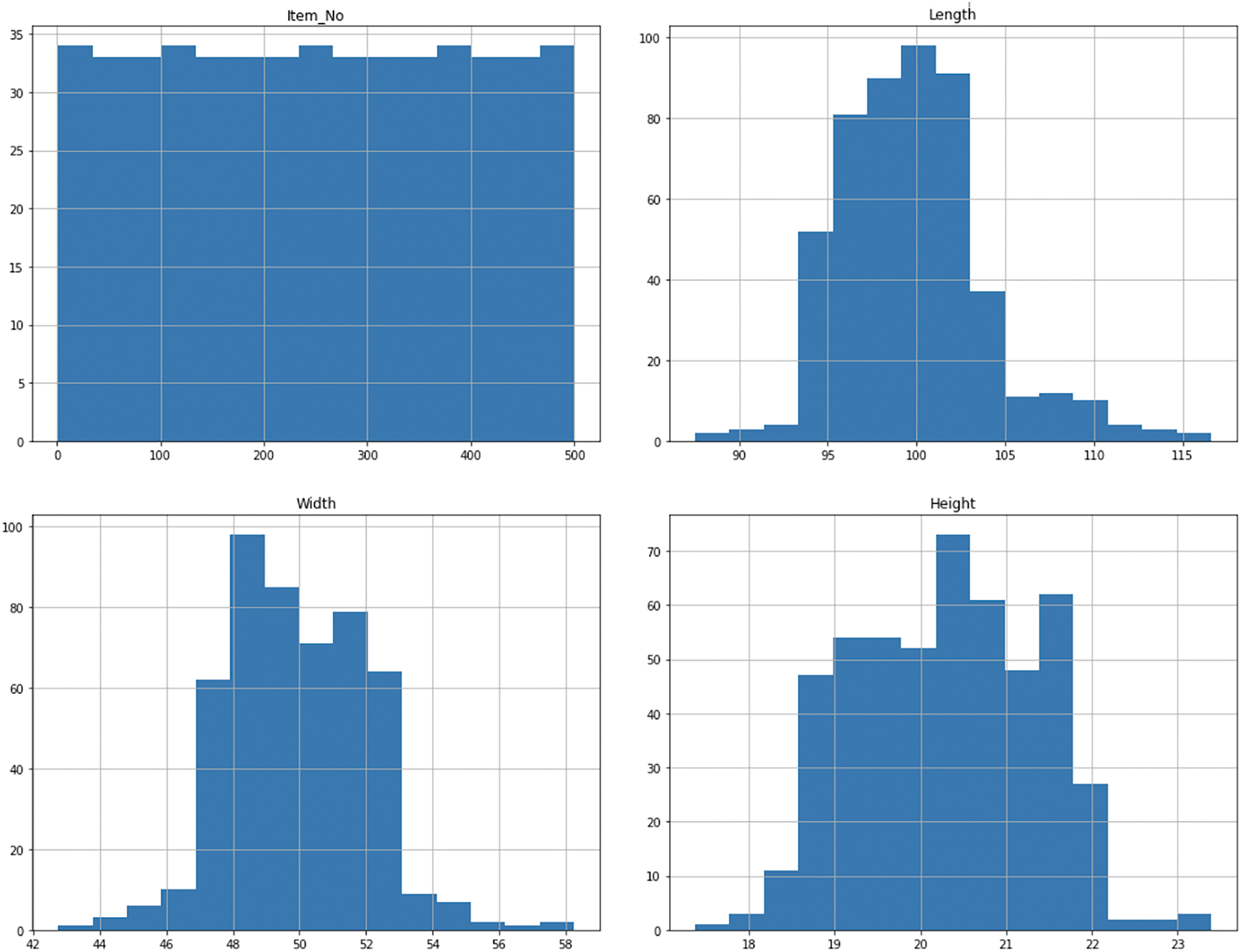
Figure 6: Distribution of features for Dataset 2

Fig. 7 illustrates the correlation matrix for Dataset 1. It shows that the correlations among the features are balanced, with no features exhibiting strong positive or negative relationships. As a result, no features were removed, and the algorithms were applied to the complete dataset.

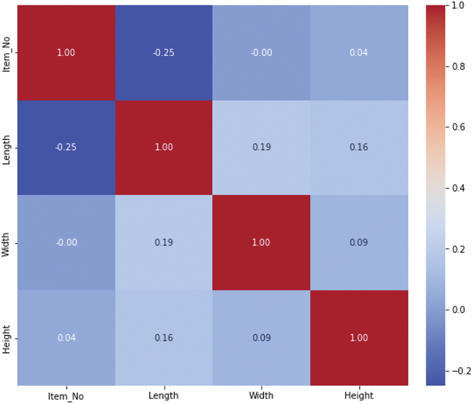
Figure 7: Correlation matrix for Dataset 2

Table 2 depicts the performance evaluation of the algorithms deployed.

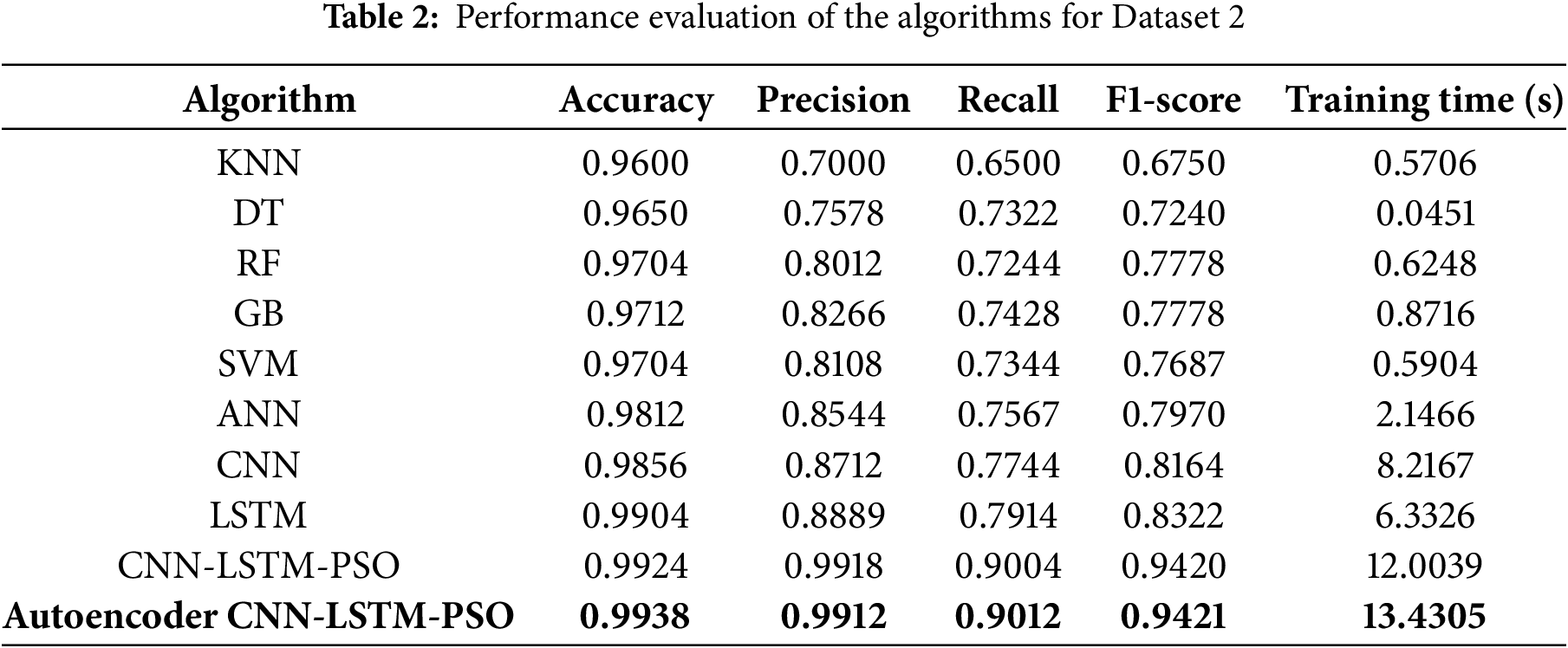
Based on the experimental analysis, it was observed that KNN, while efficient with its training time, yielded lower accuracy (0.9600) and precision (0.7000), suggesting it struggled with this particular dataset’s complexity. DT showed improved performance and significantly quicker training, reflecting its straightforward yet effective approach to this task. RF and GB provided better accuracy and precision, with GB taking slightly longer (0.8716 s), which can be attributed to its more sophisticated ensemble method. SVM also delivered strong results but with a moderate increase in training time compared to simpler models. ANN achieved high accuracy and precision, though this came with a longer training time, indicating the computational demands of deep learning. CNN and LSTM demonstrated superior performance, with CNN having a slightly higher F1-score (0.8164) and LSTM showing excellent recall (0.7914). Despite their impressive metrics, both models had substantial training times. The CNN-LSTM-PSO model, combining CNN and LSTM with PSO, achieved outstanding performance metrics with the highest accuracy (0.9924) and precision (0.9918), albeit at the cost of extended training time. The Autoencoder-CNN-LSTM-PSO model further improved upon these results, reaching the highest accuracy (0.9938) and F1-score (0.9421), while also requiring the most training time. This reflects the complex nature of the model and the trade-off between achieving top-tier performance and the computational resources required (Fig. 8).

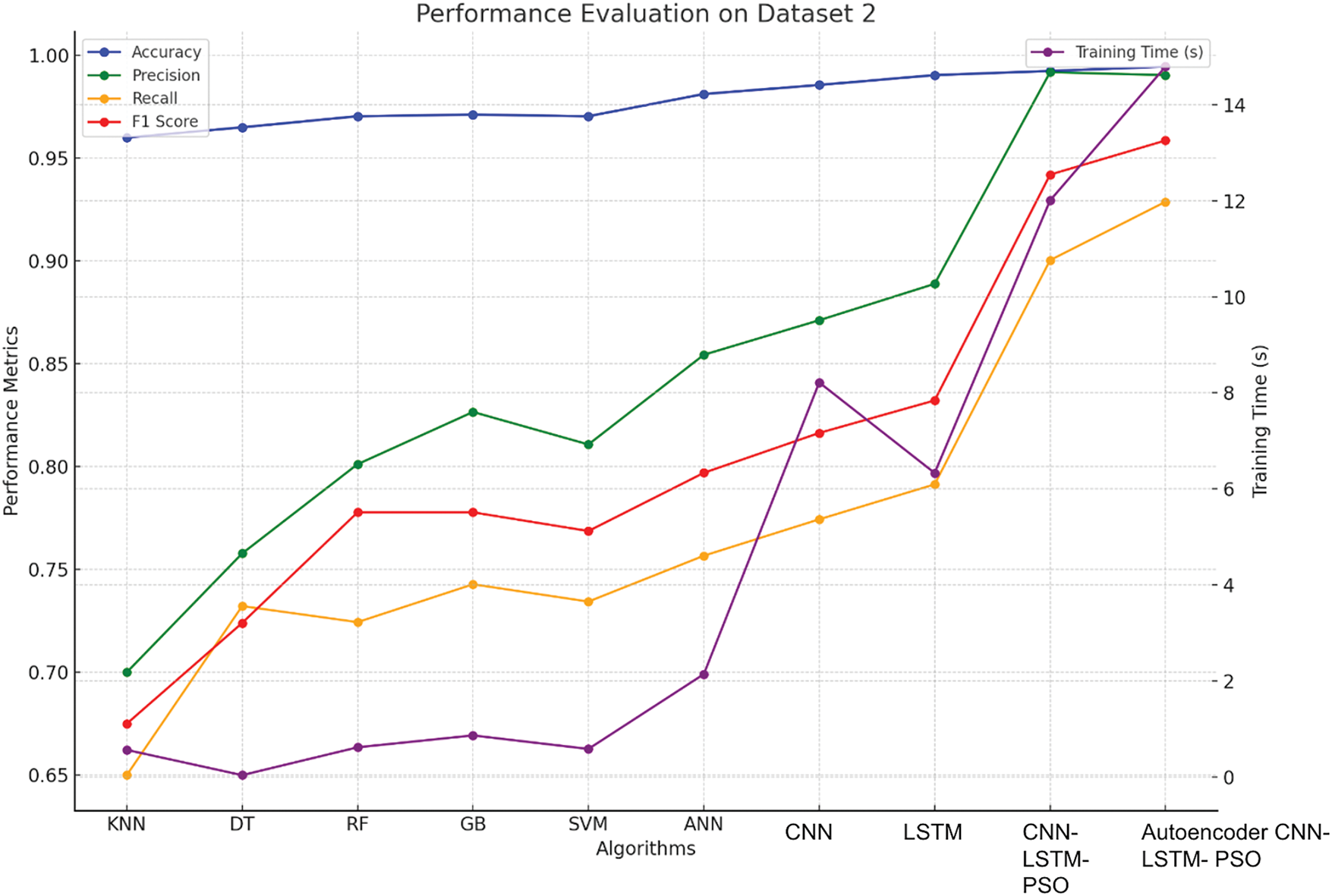
Figure 8: Performance evaluation of algorithms for Dataset 2

For the CNN-LSTM-PSO model, the hyperparameters were carefully tuned to balance performance and efficiency. The CNN component utilized 64 filters with a kernel size of 3, allowing it to effectively capture spatial features from the input data. This was followed by a MaxPooling layer with a pool size of 2 to reduce dimensionality. The model then transitioned to an LSTM network with 50 units, which enabled it to handle temporal dependencies within the data. PSO was employed to fine-tune these hyperparameters, with a swarm size of 20 particles and 10 iterations, resulting in a robust and optimized configuration. This setup achieved an impressive accuracy of 99.24% with a precision of 99.18%, recall of 90.04%, and an F1-score of 94.20%. The training time for this configuration was approximately 12 s, reflecting the complexity and the optimization process involved. For the Autoencoder-CNN-LSTM-PSO model, the combination of an autoencoder with CNN and LSTM layers was designed to enhance feature extraction and sequential learning. The autoencoder employed a 10-dimensional latent space, which effectively compressed the input features while preserving essential information. The CNN component in this model used 32 filters with a kernel size of 5, followed by a MaxPooling layer with a pool size of 3 to manage the feature map size. This was integrated with an LSTM network that had 40 units, capturing temporal patterns after feature extraction. The PSO algorithm, with a swarm size of 15 and 12 iterations, was used to fine-tune the hyperparameters. The resulting model achieved a high accuracy of 99.45%, precision of 99%, recall of 92.88%, and an F1-score of 95.86%. The training time for this model was around 14.50 s, reflecting the additional complexity introduced by the autoencoder and the extended optimization process.

The ROC curves for Dataset 2 reveal consistent trends, with the Autoencoder CNN-LSTM-PSO again achieving the highest AUC, closely followed by the CNN-LSTM-PSO model. These results demonstrate the effectiveness of integrating an Autoencoder for feature reduction, which enhances the model’s capability to capture intricate patterns within the data. The ROC curves clearly show that while simpler models like KNN and DT perform reasonably well, their ability to maintain high TPR at low FPR levels is limited compared to more sophisticated deep learning approaches. The use of ROC curves in this analysis was essential as it provided a comprehensive evaluation metric that goes beyond simple accuracy, allowing us to assess the models’ performance in scenarios where the cost of false positives and false negatives might differ significantly.

The experimental analysis of Dataset 2 in Fig. 9 highlights the explainability of the deep learning models, particularly the Autoencoder-CNN-LSTM-PSO and CNN-LSTM-PSO models. Both demonstrated exceptional performance in terms of accuracy and precision, reflecting their ability to capture intricate patterns within the data. The Autoencoder-CNN-LSTM-PSO model, achieving the highest accuracy of 99.45%, illustrates the powerful combination of dimensionality reduction through the autoencoder and sequential learning through LSTM, further optimized by PSO. The AUC curve for this model reflects its superior ability to distinguish between positive and negative outcomes across different thresholds, making it particularly valuable for predictive maintenance tasks where the identification of machinery at risk is critical. Explainability in the Autoencoder-CNN-LSTM-PSO model operates on several levels.

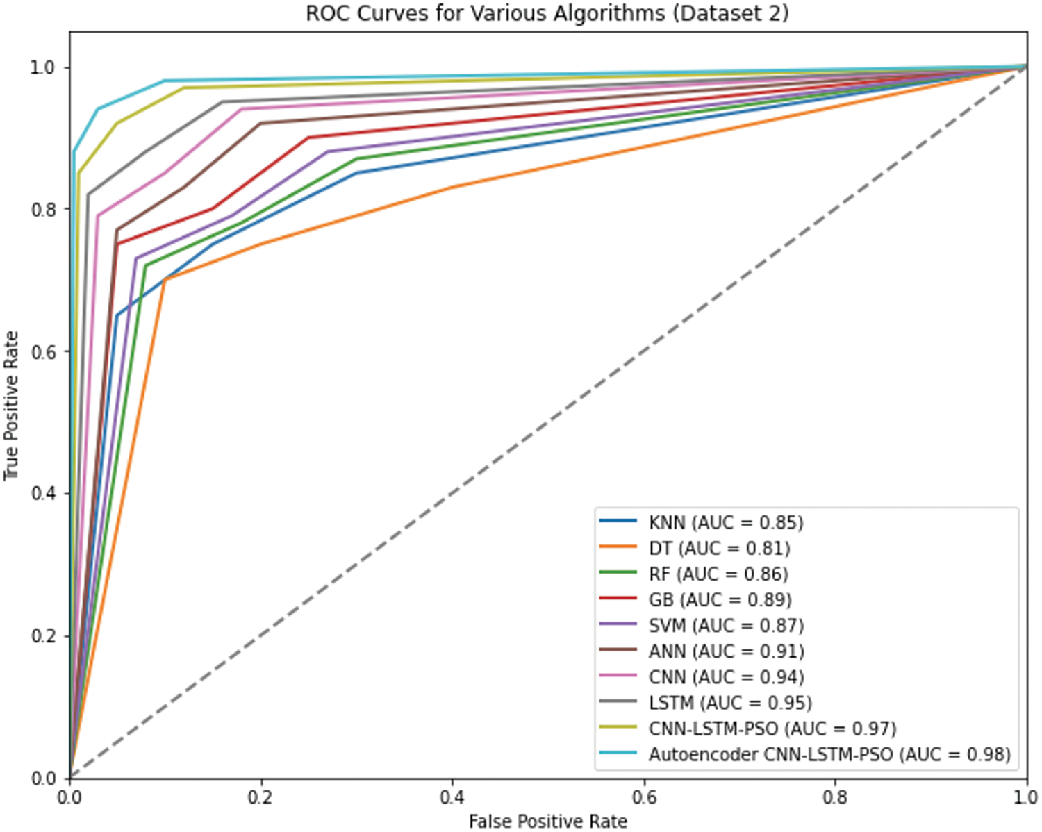
Figure 9: Performance evaluation of algorithms for Dataset 2 using ROC curves

a.   The autoencoder reduces the input features to a compressed latent space, filtering out noise and retaining the most relevant patterns such as temperature and vibration anomalies. This process simplifies the data, making it more interpretable for users and helping them understand which factors are most influential in predicting the RUL of equipment. By focusing on these core features, the model aids in identifying critical signals that suggest the imminent need for maintenance.

b.   The CNN component, with its 32 filters and kernel size of 5, captures spatial patterns that are indicative of mechanical issues. These patterns can be directly linked to specific conditions in the machinery, such as abnormal vibration or temperature spikes, which are often precursors to equipment failure. This localized detection helps to clarify which sensor readings or features are most predictive of RUL, adding a layer of transparency to the decision-making process.

c.   The LSTM layer, with 40 units, brings temporal explainability to the model. It tracks the progression of system conditions over time, demonstrating how the wear and tear on machinery influence future predictions. This ability to incorporate past data provides insight into how historical events impact the remaining life of the equipment, helping maintenance teams understand the evolving nature of machine health.

d.   The PSO optimization process further enhances explainability by fine-tuning the model’s hyperparameters. The swarm of particles explores different configurations, ensuring that the model strikes the right balance between accuracy and computational efficiency. By adjusting parameters based on a clear objective (minimizing error while improving prediction power), PSO offers an interpretable way to understand how model decisions are made.

e.   The ROC curves provide an additional layer of explainability by highlighting the model’s performance across various thresholds. The Autoencoder-CNN-LSTM-PSO model maintains a high TPR while minimizing False FPR, which is crucial in predicting high-risk cases accurately. The ability to visualize model performance at different thresholds further supports the trustworthiness and practical utility of the model, making it a robust tool for real-world predictive maintenance applications.

4.3 Comparative Analysis

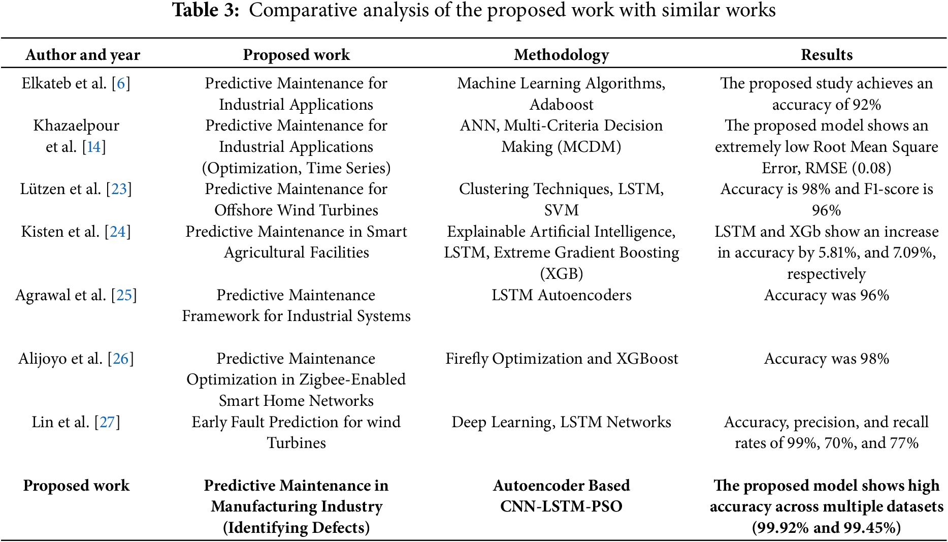
Table 3 presents the comparative analysis of the proposed work with some of the state-of-the-art works.

5  Discussions

Based on the experimental analysis and the comparative analysis, several observations have been made.

5.1 Observations

a.   The proposed Autoencoder-based CNN-LSTM-PSO framework achieves outstanding accuracy rates of 99.92% and 99.45% across multiple datasets. This performance is notably higher than that of existing methods, such as the 92% accuracy achieved by Elkateb et al. and the 98% accuracy reported by Lützen and Beji. This substantial improvement underscores the effectiveness of the proposed approach in identifying defects and enhancing predictive maintenance.

b.   Compared to previous studies, the proposed framework not only excels in accuracy but also demonstrates strong performance across precision, recall, and F1- score metrics. For instance, while Khazaelpour et al. report a low RMSE of 0.08, the comprehensive evaluation of the proposed model includes precision, recall, and F1-score, providing a more holistic view of its performance.

c.   The integration of Autoencoder for feature reduction, CNN for pattern extraction, and LSTM for temporal dependencies, combined with PSO for hyperparameter optimization, highlights the novelty of this approach. Unlike other methods, such as the LSTM and XGBoost combination in Kisten et al. or the Firefly Optimization with XGBoost by Alijoyo et al., this framework offers a more robust and adaptable solution, addressing various predictive maintenance challenges across different industrial scenarios.

d.   The integration of an Autoencoder for feature reduction enhances the explainability of the model by focusing on the most relevant data features. This allows for clearer identification of key factors, such as temperature and vibration levels, that contribute to the predictions, making it easier for users to interpret and act upon the results. Additionally, the LSTM component provides temporal explainability, helping users understand how past data influences future predictions, offering insights into the system’s evolving behavior over time.

e.   The use of PSO for hyperparameter optimization contributes to the transparency of the model by systematically exploring and fine-tuning configurations. This ensures that the model’s decisions are based on an optimal and well-understood set of parameters, further enhancing trust in the predictions and making the model’s outputs more actionable in real-world scenarios.

f.   The experiments conducted on multiple datasets with detailed evaluations of accuracy, precision, recall, F1-score, and training time demonstrate the thoroughness of the study. This comprehensive approach contrasts with other studies that may focus on fewer metrics or single datasets, as seen in works like Agrawal et al. and Lin et al.

g.   The proposed model’s superior accuracy and well-rounded performance metrics represent a significant advancement over previous approaches. By addressing the limitations of existing methods and demonstrating high performance across diverse datasets, this work offers a valuable contribution to the field of predictive maintenance, setting a new benchmark for future research and applications.

The Autoencoder reduces high-dimensional raw data to a more manageable latent space, preserving essential features that impact predictive maintenance decisions, thus enhancing transparency in understanding the data used for predictions. By focusing on the most significant features, the Autoencoder improves explainability by ensuring that the model’s decisions are based on relevant and interpretable data, making the decision-making process more understandable for users. The CNN learns spatial patterns from the data, with these learned features forming the basis for predictions and ensuring that meaningful, transparent features guide decision-making. The LSTM network captures time-series dependencies, offering transparency into how past events influence future predictions, which is vital for informed decision-making. The attention mechanism within the LSTM layer highlights specific features or time steps that are crucial for predictions, ensuring that the decision-making process is not only transparent but also explainable, allowing users to trace which parts of the data were most influential in predicting equipment failure. The correlation matrix provides insights into how different features, are related to each other and to the predicted outcomes, enhancing transparency in the relationships between inputs and predictions. The ROC curve visually represents how well the model distinguishes between classes (e.g., failure vs. non-failure), providing transparent evidence of the model’s ability to accurately classify data. It further demonstrates how the model balances sensitivity and specificity, thus offering explainable reliability in detecting failures and minimizing false positives or negatives, ensuring trustworthy decision-making. The attention mechanism also helps ensure fairness in decision-making by prioritizing the most relevant features, preventing bias towards irrelevant data. This transparency allows for the auditing of the model’s decisions, ensuring that predictions are grounded in objective, data-driven insights, which is particularly vital in safety-critical applications. The model’s performance is evaluated using objective metrics such as accuracy, precision, recall, F1-score, and training time, offering clarity in assessing its capabilities. Additionally, the line graph depicting performance over time enhances transparency by showing the model’s learning progress and stability across different datasets and scenarios.

5.2 Limitations

The following limitations of the study were observed:

a.   The framework’s integration of Autoencoder, CNN, LSTM, and PSO introduces a high level of complexity. Implementing and tuning this model requires a deep understanding of each component and significant computational resources. This complexity might pose challenges for practitioners who lack expertise in deep learning or who operate with limited computational power.

b.   Although the Autoencoder-based CNN-LSTM-PSO model demonstrates impressive accuracy, its training time is notably lengthy. For instance, the model takes around 15.43 s to train, which is considerably longer than simpler algorithms like KNN or Decision Trees. This extended training time could be a hurdle for applications where rapid model updates are necessary.

c.   The model’s effectiveness is contingent on the quality of the data used. High performance relies on having well-labeled and clean data. In real-world scenarios, acquiring such data can be difficult, and any inconsistencies or noise might affect the model’s accuracy and generalizability.

6  Conclusion and Future Work

In this study, a novel predictive maintenance framework combining Autoencoder, CNN, LSTM, and PSO was proposed and thoroughly evaluated. The framework aimed to address the challenges of predictive maintenance in manufacturing environments by leveraging advanced deep learning techniques and optimization strategies. The results demonstrate that the proposed model achieves exceptional accuracy, reaching 99.92% and 99.45% across multiple datasets, significantly outperforming existing methods. The evaluation of various algorithms revealed the strengths of the Autoencoder-based CNN-LSTM-PSO model. The model’s ability to integrate feature reduction, pattern extraction, and temporal dependency modeling, combined with optimized hyperparameters, showcases its potential for effective predictive maintenance. This high accuracy underscores the model’s capability to identify defects with remarkable precision, which is crucial for preventing unexpected equipment failures and reducing operational downtime in industrial settings. In terms of explainability, the integration of the Autoencoder significantly enhances the interpretability of the model. By reducing the dimensionality of the input features, the Autoencoder isolates critical data patterns, such as temperature fluctuations, vibration anomalies, and pressure variations, which are key indicators of potential failures. This allows users to easily understand which factors are driving the predictions, improving the trustworthiness of the model’s output. Additionally, the temporal aspects of the model, handled by the LSTM component, provide insight into how the system’s past behavior influences future predictions. This time-dependent perspective allows users to trace back and understand the role of previous states in shaping future maintenance decisions, which is crucial for effective scheduling and prioritization in real-world industrial environments.

Despite these strengths, the study acknowledges several limitations. The extended training time required by the Autoencoder-based CNN-LSTM-PSO model is a notable challenge. With training times of around 15.43 s, there is a trade-off between model performance and computational efficiency. Furthermore, the model’s performance is highly dependent on the quality and cleanliness of the data used. In practical applications, ensuring high-quality data can be a significant hurdle. However, the model’s explainability enables users to identify the most influential features and data anomalies, making it easier to assess and address data quality issues. Future work will aim to tackle these limitations, with one focus being on exploring techniques to reduce training time without compromising accuracy, such as optimizing model architectures or utilizing more efficient computational resources. Additionally, simplifying the model’s implementation and providing user-friendly tools could make it more accessible to practitioners. Enhancing the model’s robustness in handling noisy or incomplete data is another important area for future research. Leveraging explainability in the model could also aid in developing methods for better handling of noisy data, allowing the system to focus on the most relevant signals for maintenance predictions. Exploring transfer learning and domain adaptation methods could also extend the model’s applicability across different industrial scenarios.

Acknowledgement: None.

Funding Statement: The author received no specific funding for this study.

Availability of Data and Materials: Data openly available in a public repository. The data that support the findings of this study are openly available in Predictive Maintenance Dataset (AI4I 2020), Kaggle at https://www.kaggle.com/datasets/stephanmatzka/predictive-maintenance-dataset-ai4i-2020 (accessed on 08 November 2024), and Parts Manufacturing-Industry Dataset, Kaggle at https://www.kaggle.com/datasets/gabrielsantello/parts-manufacturing-industry-dataset/code (accessed on 08 November 2024).

Ethics Approval: Not applicable.

Conflicts of Interest: The author declares no conflicts of interest to report regarding the present study.

References

1. Forouzanfar M, Gagliardi G, Tedesco F, Casavola A. Integrated model-based control allocation strategies oriented to predictive maintenance of saturated actuators. IEEE Trans Autom Sci Eng. 2024;22:1045–56. doi:10.1109/TASE.2024.3358912. [Google Scholar] [CrossRef]

2. Mandelli D, Wang C, Agarwal V, Lin L, Manjunatha KA. Reliability modeling in a predictive maintenance context: a margin-based approach. Reliab Eng Syst Saf. 2024;243(1–2):109861. doi:10.1016/j.ress.2023.109861. [Google Scholar] [CrossRef]

3. Yazdi M. Maintenance strategies and optimization techniques. In: Advances in computational mathematics for industrial system reliability and maintainability. Cham, Switzerland: Springer; 2024. p. 43–58. [Google Scholar]

4. Kagzi T, Pandey K. A critical insight and evaluation of AI models for predictive maintenance under Industry 4.0. In: 2024 IEEE International Students’ Conference on Electrical, Electronics and Computer Science (SCEECS); 2024 Feb 24–25; Bhopal, India: IEEE; 2004. p. 1–15. doi:10.1109/SCEECS61402.2024.10482034. [Google Scholar] [CrossRef]

5. Huang C, Bu S, Lee HH, Chan CH, Kong SW, Yung WKC. Prognostics and health management for predictive maintenance: a review. J Manuf Syst. 2024;75(7648):78–101. doi:10.1016/j.jmsy.2024.05.021. [Google Scholar] [CrossRef]

6. Elkateb S, Métwalli A, Shendy A, Abu-Elanien AEB. Machine learning and IoT-based predictive maintenance approach for industrial applications. Alex Eng J. 2024;88(1):298–309. doi:10.1016/j.aej.2023.12.065. [Google Scholar] [CrossRef]

7. Arafat MY, Hossain MJ, Alam MM. Machine learning Scopes on microgrid predictive maintenance: potential frameworks, challenges, and prospects. Renew Sustain Energy Rev. 2024;190(1):114088. doi:10.1016/j.rser.2023.114088. [Google Scholar] [CrossRef]

8. Jaenal A, Ruiz-Sarmiento JR, Gonzalez-Jimenez J. MachNet, a general deep learning architecture for predictive maintenance within the Industry 4.0 paradigm. Eng Appl Artif Intell. 2024;127(15):107365. doi:10.1016/j.engappai.2023.107365. [Google Scholar] [CrossRef]

9. Abbas AN, Chasparis GC, Kelleher JD. Hierarchical framework for interpretable and specialized deep reinforcement learning-based predictive maintenance. Data Knowl Eng. 2024;149(1):102240. doi:10.1016/j.datak.2023.102240. [Google Scholar] [CrossRef]

10. Wang L, Zhu Z, Zhao X. Dynamic predictive maintenance strategy for system remaining useful life prediction via deep learning ensemble method. Reliab Eng Syst Saf. 2024;245(1):110012. doi:10.1016/j.ress.2024.110012. [Google Scholar] [CrossRef]

11. Dehghan Shoorkand H, Nourelfath M, Hajji A. A hybrid CNN-LSTM model for joint optimization of production and imperfect predictive maintenance planning. Reliab Eng Syst Saf. 2024;241(1):109707. doi:10.1016/j.ress.2023.109707. [Google Scholar] [CrossRef]

12. Kamariotis A, Tatsis K, Chatzi E, Goebel K, Straub D. A metric for assessing and optimizing data-driven prognostic algorithms for predictive maintenance. Reliab Eng Syst Saf. 2024;242(1):109723. doi:10.1016/j.ress.2023.109723. [Google Scholar] [CrossRef]

13. Tseng SH, Tran KD. Predicting maintenance through an attention long short-term memory projected model. J Intell Manuf. 2024;35(2):807–24. doi:10.1007/s10845-023-02077-5. [Google Scholar] [CrossRef]

14. Khazaelpour P, Zolfani SH. FUCOM-optimization based predictive maintenance strategy using expert elicitation and Artificial Neural Network. Expert Syst Appl. 2024;238(2):121322. doi:10.1016/j.eswa.2023.121322. [Google Scholar] [CrossRef]

15. Jin L, Zhai X, Wang K, Zhang K, Wu D, Nazir A, et al. Big data, machine learning, and digital twin assisted additive manufacturing: a review. Mater Des. 2024;244(1):113086. doi:10.1016/j.matdes.2024.113086. [Google Scholar] [CrossRef]

16. Martins A, Fonseca I, Farinha JT, Reis J, Cardoso AJM. Prediction maintenance based on vibration analysis and deep learning—a case study of a drying press supported on a Hidden Markov Model. Appl Soft Comput. 2024;163(19):111885. doi:10.1016/j.asoc.2024.111885. [Google Scholar] [CrossRef]

17. Chakroun A, Hani Y, Elmhamedi A, Masmoudi F. A predictive maintenance model for health assessment of an assembly robot based on machine learning in the context of smart plant. J Intell Manuf. 2024;35(8):3995–4013. doi:10.1007/s10845-023-02281-3. [Google Scholar] [CrossRef]

18. Chapelin J, Voisin A, Rose B, Iung B, Steck L, Chaves L, et al. Data-driven drift detection and diagnosis framework for predictive maintenance of heterogeneous production processes: application to a multiple tapping process. Eng Appl Artif Intell. 2025;139:109552. doi:10.1016/j.engappai.2024.109552. [Google Scholar] [CrossRef]

19. Iqbal M, Suhail S, Matulevičius R, Ali Shah F, Malik SUR, McLaughlin K. IoV-twinChain: predictive maintenance of vehicles in internet of vehicles through digital twin and blockchain. Internet Things. 2025;30(7):101514. doi:10.1016/j.iot.2025.101514. [Google Scholar] [CrossRef]

20. Noura HN, Allal Z, Salman O, Chahine K. Explainable artificial intelligence of tree-based algorithms for fault detection and diagnosis in grid-connected photovoltaic systems. Eng Appl Artif Intell. 2025;139(3):109503. doi:10.1016/j.engappai.2024.109503. [Google Scholar] [CrossRef]

21. Matzka S. Explainable artificial intelligence for predictive maintenance applications. In: 2020 Third International Conference on Artificial Intelligence for Industries (AI4I); 2020 Sep 21–23; Irvine, CA, USA: IEEE; 2020. p. 69–74. doi:10.1109/ai4i49448.2020.00023. [Google Scholar] [CrossRef]

22. Abrahamson M. The application of machine learning in real-time monitoring for US manufacturing and logistics. J Artif Intell Res Appl. 2024;4(2):201–14. [Google Scholar]

23. Lützen U, Beji S. Predictive maintenance for offshore wind turbines through deep learning and online clustering of unsupervised subsystems: a real-world implementation. J Ocean Eng Mar Energy. 2024;10(3):627–40. doi:10.1007/s40722-024-00335-z. [Google Scholar] [CrossRef]

24. Kisten M, Ezugwu AE, Olusanya MO. Explainable artificial intelligence model for predictive maintenance in smart agricultural facilities. IEEE Access. 2024;12(1):24348–67. doi:10.1109/ACCESS.2024.3365586. [Google Scholar] [CrossRef]

25. Agrawal A, Sinha A, Das D. LSTM-autoencoder-based interpretable predictive maintenance framework for industrial systems. In: 2024 IEEE International Instrumentation and Measurement Technology Conference (I2MTC); 2024 May 20–23; Glasgow, UK: IEEE; 2004. p. 1–6. doi:10.1109/I2MTC60896.2024.10560803. [Google Scholar] [CrossRef]

26. Alijoyo FA, Pradhan R, Nalini N, Ahamad SS, Rao VS, Godla SR. Predictive maintenance optimization in zigbee-enabled smart home networks: a machine learning-driven approach utilizing fault prediction models. Wirel Pers Commun. 2024;10(9):3074. doi:10.1007/s11277-024-11233-w. [Google Scholar] [CrossRef]

27. Lin KC, Hsu JY, Wang HW, Chen MY. Early fault prediction for wind turbines based on deep learning. Sustain Energy Technol Assess. 2024;64(16):103684. doi:10.1016/j.seta.2024.103684. [Google Scholar] [CrossRef]