A Novel Stacked Network Method for Enhancing the Performance of Side-Channel Attacks

1  Introduction

Side-channel Analysis (SCA) represents a powerful cryptographic algorithm attack. The adversary exploits the information leaked from the physical implementation to target the secret key. During this attack, the adversary attempts to recover certain information related to the secret key. In recent years, there has been increasing attention paid to using the DL-SCA method for cryptographic attacks. This method can transform the traditional SCA into a classification problem. Therefore, an increasing number of scholars have conducted extensive research, which involves mathematical analysis methods and the construction of deep learning networks, to reveal cryptographic keys.

Currently, there are two main types of SCA: profiled SCA [1,2] and non-profiled SCA [3,4]. The former is the most powerful type of SCA. In the profiled SCA, the adversary can establish a mathematical model by collecting sensitive information, such as power consumption leaked from the target device. Subsequently, in the attack phase, they use the established model to execute the attack. Common methods include template attacks [5] and simple power attacks [6]. On the other hand, non-profiled SCA refers to the adversary directly performing operations on the target device and referring to the key by exploiting the leaked side-channel information. During the implementation process, the adversary can conduct attacks by collecting the power consumption information leaked from each plaintext. Moreover, they can obtain the key by calculating the correlation between the leakage points and the sensitive data. Such attack methods mainly include correlation power analysis [7], electromagnetic attack [8], and others. All of these methods use some mathematical analysis techniques to directly obtain the secret key.

Through the survey of relevant works in recent years, DL-SCA research has received widespread attention. Since Maghrebi et al. [9] first proposed using deep learning to perform complex SCA, this field has attracted significant interest from researchers. Many methods aim to build new models for analyzing [10–12], leveraging the powerful learning abilities of these models to better capture the efficient features in the dataset. For the complete traces of long time series, successful attacks can be achieved using the window trimming technique [13–15], where the window is typically selected from the location of the leakage. This method alleviates the effort required by the model. Most importantly, pre-selection techniques are usually preferred when working with protected datasets. Additionally, Perin et al. [16] proposed a metric to indicate when the model converges. Zhang et al. [17] introduced a new loss function to evaluate the performance of deep learning models in the context of SCA. The study shows that this metric can significantly improve attack efficiency when dealing with data imbalance problems. Remarkably, study [18] is the first end-to-end deep learning attack implemented on complete power consumption traces, without any preprocessing techniques, and the model complexity is unimaginable. However, this method is not the optimal solution for the attack, especially when encountering datasets with high noise and strong protective countermeasures.

Recently, ensemble learning methods have been introduced into SCA research. Authors in [19] used Bagging is used to improve the output class probability of the models, achieving better attack performance by integrating several trained models. The authors of [20] proposed a CNNP model, a variant of CNN, to reduce the application requirements of deep learning in SCA. Although existing research has made significant progress in deep learning and ensemble learning methods, there are still some research gaps for improvement. First, there is a lack of research on the interpretability of Stacking integration, and the internal framework logic remains insufficiently explained. Second, current research mainly focuses on standard datasets and has not yet covered a wider range of practical application scenarios. Adapting ensemble learning methods to different hardware platforms remains a challenge that needs to be overcome. Therefore, this paper proposes a SCA method based on a Stacking ensemble, called Stacking-SCA. Our method further explores the extended application of the base models and meta-model in Stacking. Next, the internal structure of the Stacking is optimized, and the original ASCAD database is divided into five subsets as mutually independent multi-segment datasets. Experiments are conducted on multiple hardware platform datasets to verify the feasibility and robustness of the method.

The contribution of this paper is as follows:

•   Introducing an ensemble method called Stacking-SCA. This method improves the generalization capability of models through deep model integration, exploring its potential in side-channel analysis. Stacking-SCA comprehensively expands the base models and meta-model, fully demonstrating the advantages of integrating multiple deep learning models.

•   Adopting an alternative strategy to optimize the cross-validation process. Specifically, our method demonstrates that extracting five subsets from the original ASCAD database as inputs to Stacking-SCA can improve model generalization.

•   Conducting extensive experimental analysis and comparisons on three publicly hardware platform datasets. Compared to related state-of-the-art works and other ensemble techniques, our approach demonstrates superior performance in key recovery.

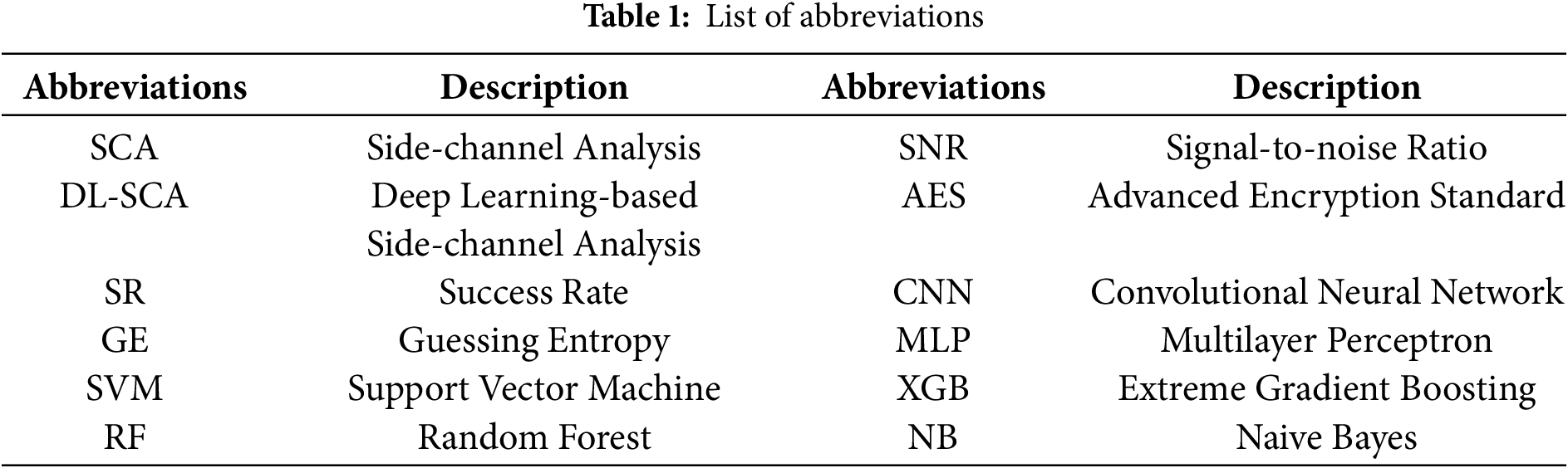
The rest of the paper is structured as follows: Section 2 discusses the datasets of our experiments, SCA and deep learning, and ensemble methods. In Section 3, the Stacking-SCA method and the multi-segment datasets are discussed. Moreover, the structural design of the base model and the meta-model are also given in detail. Section 4 provides experimental results on three datasets and compares them with some state-of-the-art works. Finally, Section 5 concludes the paper and provides some potential future research directions. Table 1 lists the abbreviations used in this paper.

2  Background

2.1 Ensemble Methods in Machine Learning

Boosting: This type of ensemble is suitable when there are dependencies between individual learners, requiring a sequential generation and serialization method. Its main working principle involves training a base learner from an initial training set, and adjusting the sample distribution based on the performance of the base learner. Finally, it produces a classifier with optimal metrics selected from the training data.

Bagging: It is considered a collective ensemble learning algorithm in the field of machine learning, which can be combined with other classification and regression algorithms. This method involves the averaging or linear combination of the predictions from individual classifiers. Bagging helps reduce the variance among different classifiers and avoids the risk of overfitting.

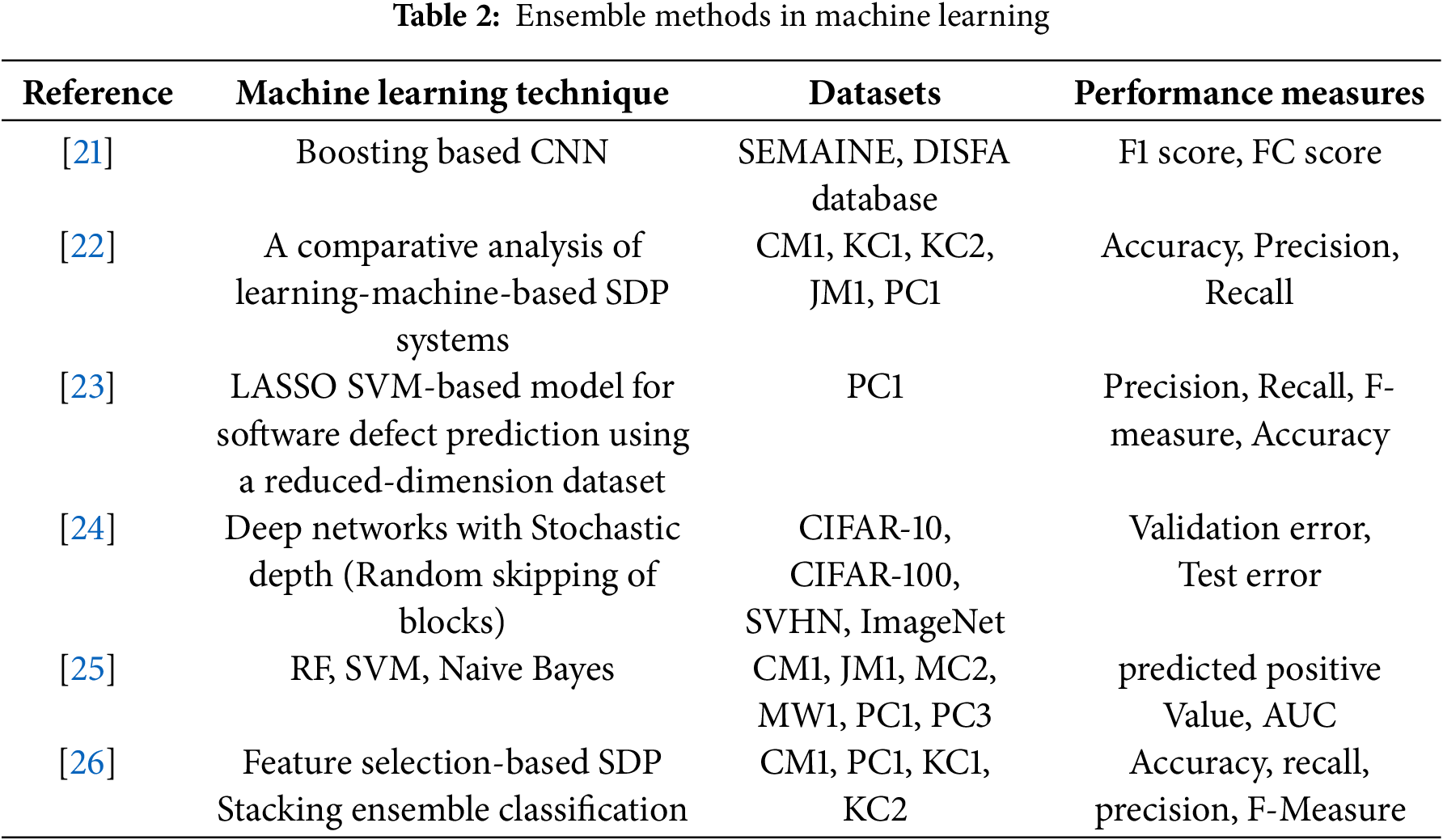
Stacking: This method mainly involves training several base models and combining them into a meta-model to enhance predictive performance. In the first stage, the dataset is divided through cross-validation and used to train base classifiers. In the second stage, a meta-level classifier is trained to combine the output of the base classifiers. Moreover, the Stacking method reduces bias and improves generalization compared to using a single learning algorithm. Stacking commonly uses several types of base models to build different predictors. The meta-model can be any machine learning model, such as neural networks, and others. The goal of the meta-model is to combine the prediction results of different base models and optimize the overall predictive performance. Table 2 shows the ensemble methods used in machine learning.

2.2 Profiled Deep Learning Side-Channel Attacks

The application of deep learning to perform profiling side-channel attacks is analyzed. Firstly, the attacker requires access to a pair of identical devices, called the target device and profiling device. The target device performs the encryption operation. In this process, the attacker collects sensitive information leaked from the implementation for analysis. This is specifically represented as follows:

•   Profiling device: The attacker acquires side-channel traces from this device and collects information about intermediate calculations leaked during the encryption operation. They mainly analyze the power consumption associated with all possible hypothetical key values.

•   Target device: The attacker categorizes the input traces to fully recover the key based on the sensitive information.

In the profiling phase of SCA, the deep learning network utilizes random variables X (side-channel traces) and features F as inputs. According to the training rules of the neural network, side-channel traces are classified based on the corresponding key value, and the class label Y is estimated to obtain the output probability pi,j. The label of each trace i is calculated by the function f(Pi, K) of the leakage model, where Pi represents the input plaintext and K represents the random key (K [0, 255]). Inputting N side-channel traces, the deep neural network outputs the maximum sum of candidate probabilities Sk, corresponding to the correct key, which is defined as follows:

(1)

The value pi,j represents the probability of key k, achieved by using the attack trace, leakage model, and input data (corresponding to the input of each hypothesis value).

2.2.1 Metric

In the attack phase, the attacker collects an attack set of size Q, consisting of plaintext inputs and corresponding attack traces. Typically, the adversary does not focus on the training and attacking phase, their main goal is to recover the secret key. The commonly used metrics are success rate (SR) and guessing entropy (GE). This paper mainly uses the GE for evaluation. The GE metric is defined as follows:

(2)

where k* is the correct key, a denotes the number of attacks, and g denotes the key guessing vector, denoted as g = [g1,g2, … , g|k|]. The average position of k* in g is determined by ranking the predicted values. In our experiments, the dataset is randomly shuffled 100 times, and compute the average GE value to obtain significant results.

2.2.2 Solution

To address the challenges encountered in Profiled DL-SCA, the following strategies are proposed:

(1) Data Preprocessing

In the presence of facing complex and noisy side channel data, preprocessing techniques can be applied to reduce the impact of external factors. Standardization, normalization, and denoising procedures help mitigate the effects of noise, improving the convergence speed and training stability of the model.

(2) Feature Engineering

Feature engineering techniques can be used to remove irrelevant or redundant features, thereby reducing the model’s susceptibility to noise or adversarial attacks. Methods such as principal component analysis (PCA) and Linear Discriminant Analysis (LDA) can help retain important signal features and reduce the complexity of attacks.

(3) Hyperparameter Tuning and Model Selection

Hyperparameter tuning plays a crucial role in enhancing the robustness of DL-SCA. By accurately adjusting hyperparameters such as learning rate, batch size, and regularization coefficient, the robustness of the model against noise and interference is improved. Tuning hyperparameters across different datasets has significantly improved the generalization ability of the model.

2.3 Dataset

2.3.1 ASCAD

The ASCAD [27] dataset consists of measurement values obtained from an 8-bit AVR microcontroller, which implements the masked AES-128 algorithm. It contains two types: one with random keys and random plaintexts, comprising a total of 200,000 traces for analysis and 100,000 traces for attack. Each trace in this dataset contains 1400 features. The second one consists of the fixed key and random plaintexts, with 50,000 traces used for profiling and 10,000 traces for attacking. Each trace in this dataset has 700 features. Additionally, the third key byte is attacked according to the choice of the leakage model.

2.3.2 DPAV4

The DPAv4 [28] contains measurements obtained from the implementation of AES-256 RSM (rotated S-box). It consists of 34,000 power traces with a fixed key and first-order masking. Each trace in this dataset contains 2000 features. It is an AES software implementation where most of the leakage operations are caused by S-box operations, rather than register writes. The mask is known, therefore it is considered an unprotected dataset. For convenience, we select the first round of S-box operation for the attack.

2.3.3 AES_HD

This dataset [29] is implemented on the unprotected AES-128 algorithm on the target device Xilinx Virtex-5 FPGA, as part of the SASEBO GII SCA evaluation board. This dataset includes 75,000 measurements, with the training set containing 50,000 traces and the attack set containing 25,000 traces. Each trace consists of 1250 features. The Hamming distance leakage model targets the last round register writes and performs attacks on the first byte.

3  Methodology

3.1 Model Ensembles with Stacking-SCA

Generally, the generalization capability of a model directly affects the successful key recovery. In the domain of SCA, test accuracy is commonly used as the criterion for evaluating generalization. Therefore, neural networks with very high test accuracy represent strong generalization ability. The generalization phase starts when the training set reaches sufficient accuracy. This phase may start soon after training or take a long time to reach. Interestingly, metrics such as key ranking, and success rate, are used as evaluation criteria, but they are difficult to accurately evaluate during the training phase.

The most significant factor is the output class probability of the model, which represents the probability of each key in the test set. In practice, this metric demonstrates good effectiveness and feasibility. If the model achieves sufficiently good generalization, the maximum output class probability corresponding to the correct key byte becomes higher. Therefore, in order to achieve this goal, a Stacking method based on SCA is introduced, called Stacking-SCA. In contrast to Bagging, it adopts the cross-validation structure and a meta-model. The advantages are very significant. This method enhances the model’s generalization and stability by effectively capturing the complex structure of the data through the stacking and combination of deep learning models.

In this method, the two core concepts of the base model and the meta-model are used, and their definitions are as follows:

•   Base model: The base model is the basic component of the stacking ensemble method, called the first layer model. It usually consists of multiple independently trained models (such as decision trees, support vector machines, neural networks, etc.). These base models make predictions by learning from different features or subsets of the data. This method improves the overall performance by combining the prediction results of these models.

•   Meta-model: As the second-layer model, the meta-model takes the prediction results of the base models as input to generate the final prediction. The meta-model usually uses a simple model (such as MLP) for prediction. During the training process, the meta-model does not directly train the original data, but uses the prediction results of the base model as input for secondary training to learn to combine these prediction results.

For a very large training set, increasing the number of models undoubtedly introduces complexity. Note that the hyperparameter architectures of the neural network are not extensively considered, which requires substantial time and computational resources. One might be concerned about whether the presence of poorly performing models in training would have a significant impact on the generalization of the overall model. What’s more, in ensemble approaches, multiple models are integrated. For underperforming models, the effects introduced by these models will be removed by models with generalization. This illustrates that the integration of multiple models in the ensemble, such as five models, can significantly improve performance.

Assuming each model outputs the class probability as p(x|y), k represents the number of models, the final ensemble prediction for m models can be expressed as:

(3)

Supposing a set of i base models M1,M2, … , Mi, and the predicted values of the i base models on the test set, denoted as t1,t2, … , ti. Let v1,v2, … ,vj denote the predicted values on the validation set. Then, the training set Xtra to train the base models. The Dtra represents the training inputs to the meta-model, which is defined as follows:

(4)

The test set of meta-model is denoted as Dtest, where k represents the number of base models. Then, let us denote the Dtest vector that relates to the average values of the base model test weights, such that

(5)

Next, the above Eq. (3) is modified, as it does not reflect the situation when the best model outputs. The modified key ranking of class output probabilities provides richer information about the generalization ability of the model. Here, mt represents the meta-model. Based on the generated Dtra and Dtest, the overall probability obtained after multiple integrations is calculated as follows:

(6)

In Eq. (6), where argmin (Dtra, mt, Dtest) refers to output probability values computed on the test set, Dtest, after training the mt with the training set Dtra.

The Stacking-SCA training process can be divided into two main steps:

1. Data partitioning and base model training. First, the selected dataset is divided into training and test sets, typically using K-fold cross-validation. In each fold, the training dataset is split into K subsets, where K-1 subsets are used as training sets to train multiple base models. The remaining single subset is used as the test set, and the prediction results of the base models on the test set are used to evaluate the performance of the base learners.

2. Meta-model training and testing. In this stage, the base model prediction and the corresponding true labels are combined as the training input of the meta-model. This training set contains the original features and incorporates the prediction results of the base models as new features. Additionally, an independent validation set is used. The validation set is predicted using the base models in the same manner as in the first step. Note that there is no need to perform any processing of the validation set, and predict all the data each time. The predictions from the base models are combined to generate the final output class probabilities for each hypothesis key in the meta-model.

Fig. 1 shows the framework of our Stacking-SCA method. In the figure, the power consumption traces and labels are used as inputs, which are divided into training and test sets through cross-validation. The base models of different architectures are represented as M1, M2, … , Mk, but they are not significantly different in the graph. Dtra and Dtest are used for meta-model training and testing. Specifically, the Dtra is used to train the meta-model, and Dtest to generate the final prediction results. The predicted vector values are denoted by P1, P2, … , Pk. In the process of meta-model, it corresponds to the representation in Eq. (6).

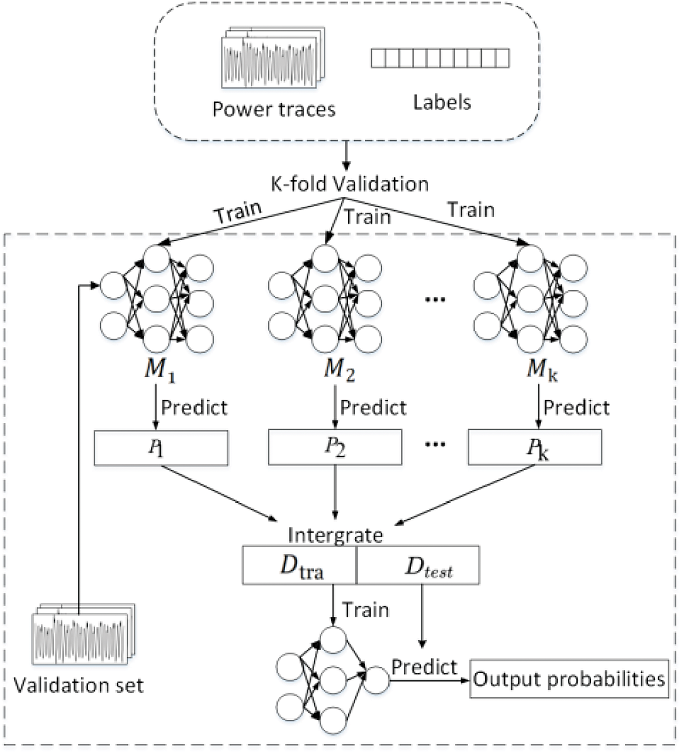
Figure 1: Stacking-SCA framework

3.2 The Multi-Segment Datasets for Stacking-SCA

Note that in the context of neural networks, it’s crucial for each model’s training set to be distinct, enabling the learning of diverse features. If the training sets exhibit similarities, the neural network could learn similar representations from these sets, potentially impacting the performance of the overall model. In the cross-validation phase of Stacking-SCA, it is unavoidable that subsets with similar data distributions will be used for training the base models. In this case, the meta-model may excessively depend on these similar prediction results, thereby increasing the risk of overfitting. To address this problem, multi-segment datasets are used as inputs, comprising mutually independent subsets. Simultaneously, the cross-validation phase is omitted. The motivation for these multi-segment datasets is derived from the dataset selection and mathematical analysis method proposed by Ou et al. [30] in their study. Five subsets with a sufficiently high signal-to-noise ratio (SNR) are extracted from the original ASCAD database as inputs for the Stacking-SCA. The high SNR implies that the attacker can extract useful information from the side channel more easily, facilitating attacks and acquisition of sensitive data. Among these, employing the five-fold cross-validation is widely considered a balanced choice.

Getting the power traces Ti and the label V, the SNR for each dimension is calculated according to the SNR formula as follows:

(7)

where Ti represents the i-th column of the original traces T, and each column has 60,000 dimensions. The Ti is divided into 256 different categories according to the middle-value V, then calculate the expectation and variance of each category. Moreover, the variance expectation and expected variance are computed respectively, and the SNR result is obtained by dividing the two.

In Fig. 2, the first subplot illustrates the overall SNR analysis results of the original ASCAD power traces. The subsequent five subplots, from the second to the sixth, show the results of the selected datasets within the five peak ranges in the first subplot, respectively. Each peak interval includes 700-dimensional power consumption. This training approach differs from the previous Stacking-SCA procedure. With traditional cross-validation, significant differences in data distribution among the five subsets may lead to inconsistent performance of the base models, thereby affecting the overall prediction quality of the meta-model. Therefore, the cross-validation process is optimized. Specifically, an alternative strategy is used by using five subsets with substantial information as input to achieve the effect of cross-validation. The different input subsets provide diverse perspectives and features, allowing the meta-model to more effectively integrate the diverse outputs of the base models. Each subset is divided into two parts with a ratio of 4:1 for training the base models, where one part is used as the training set and the other as the test set. Each subset is dedicated to training a base model. Finally, the predictions are collected from the five base models as input to the meta-model.

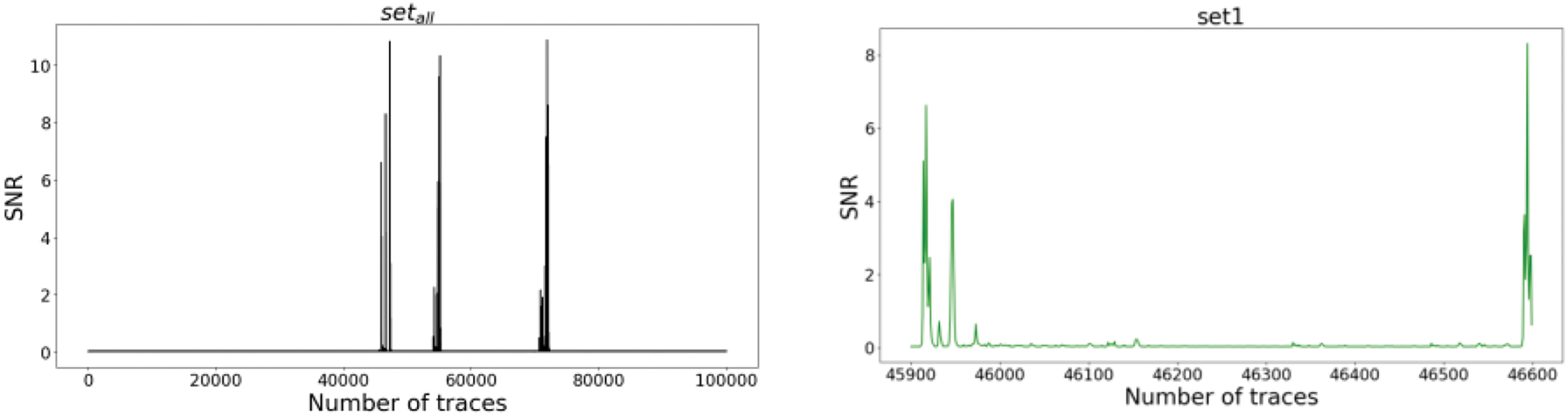
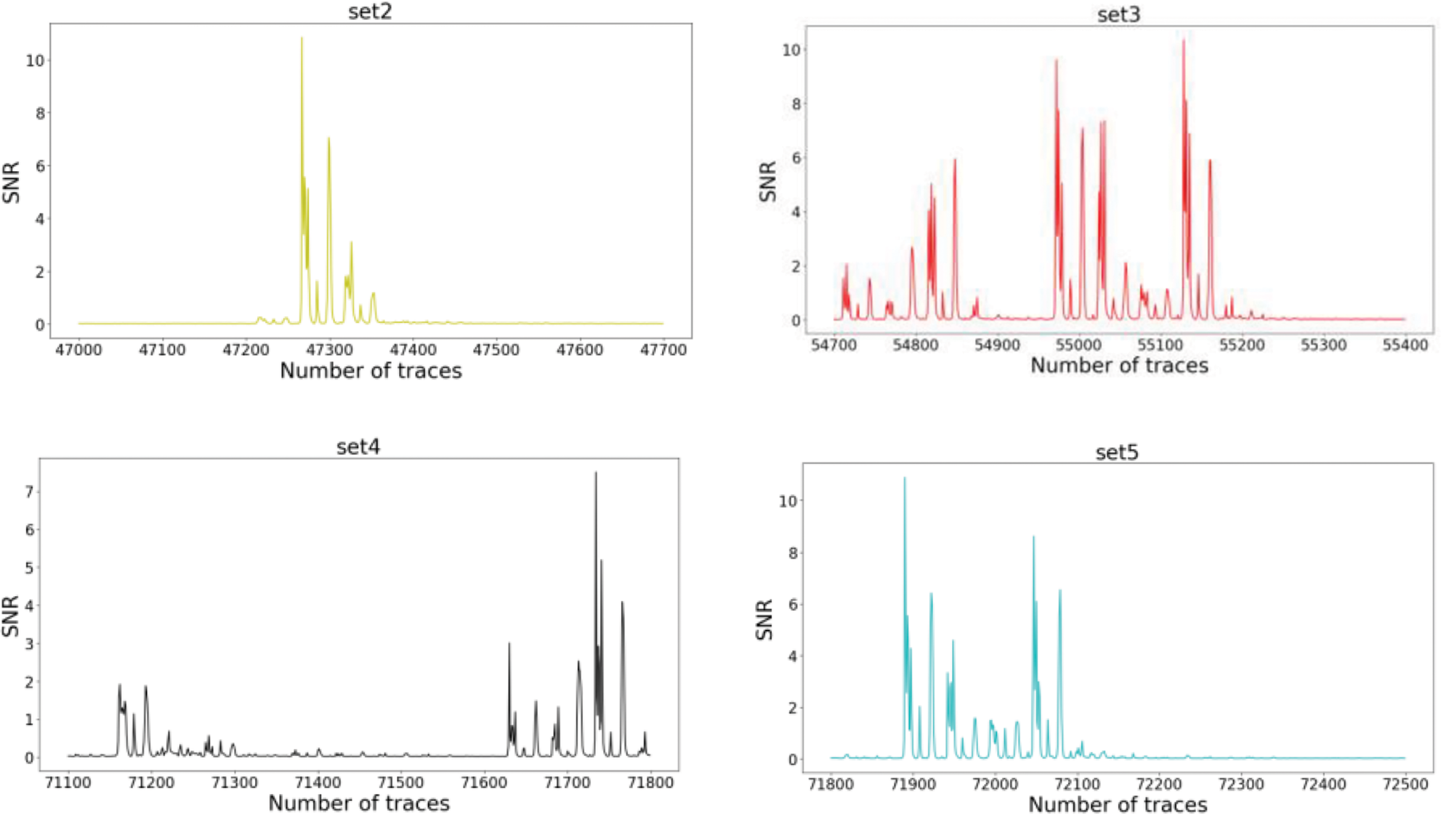
Figure 2: Setall is the total SNR result, set1 to set5 are the SNR results from the five peak intervals in setall, respectively

3.3 Model Architecture Design

3.3.1 Base Model Design

The CNN is the basic component of the base model, which is widely used in various fields. CNN is selected as the base model primarily due to its outstanding performance in processing high-dimensional and complex spatial data structures, allowing it to efficiently extract features with fewer parameters. Fig. 3 illustrates the overall architecture of the CNN. Each convolutional block consists of a one-dimensional convolutional layer, a batch normalization layer, and a one-dimensional pooling layer. Inputting the power traces, the base models calculate the base predictions, which are used as inputs for the meta-model. Moreover, in the base model design, a batch normalization layer is adopted between the convolutional layer and pooling layer to normalize the inputs, improving the network stability and convergence speed.

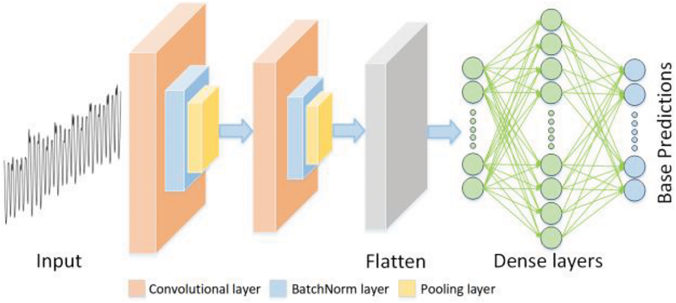
Figure 3: The CNN architecture

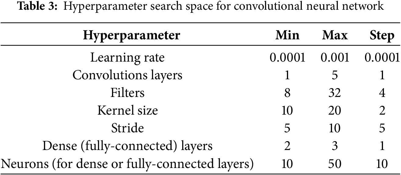
Note that CNN models [31] are used as base models under different constraint conditions. The hyperparameters of the base models are randomly selected from the predefined ranges listed in Table 3. The design of CNN models and the selection of hyperparameters are crucial in deep learning, as they directly affect the model performance and generalization ability. These ranges are determined based on the results of related works. For the selection of the learning rate, its importance in gradient descent optimization is considered. Therefore, the learning rate is set within the range of 0.0001 to 0.001. A strategy of increasing the convolution kernel size is adopted. Specifically, the kernel size is always twice that of the previous layer. This design allows the model to capture feature patterns over a larger range while maintaining local features. The number of convolutional blocks is randomly selected from {1,2,3,4,5}. The fully connected layers consist of many neurons, with their quantities randomly chosen from {10,20,30,40,50}. In the design of hyperparameter architecture, certain parameters are fixed to reduce the search space and simplify the experimental design. For the optimizer, the Adam optimizer is used, and the weight initialization adopts the He uniform method.

3.3.2 Meta-Model Design

The architecture of the MLP [19] used in this work is shown in Fig. 4. The MLP serves as the basic component of the meta-model in Stacking-SCA. The goal of the meta-model is to combine the predictions of multiple base models to generate the final prediction, rather than independently learning complex patterns. It consists of an input layer, an output layer, and several hidden layers. The design structure of the meta-model is relatively simple. In the input layer, the predictions from the base models serve as the input features to the meta-model, with a feature dimension of 256. “BN” denotes the batch normalization operation. The intermediate fully connected layers consist of three layers with ReLU activation, with sizes of 512, 512, and 256, respectively. The output layer has 256 dimensions, representing the probability corresponding to each intermediate value, serving as the predictions of the meta-model.

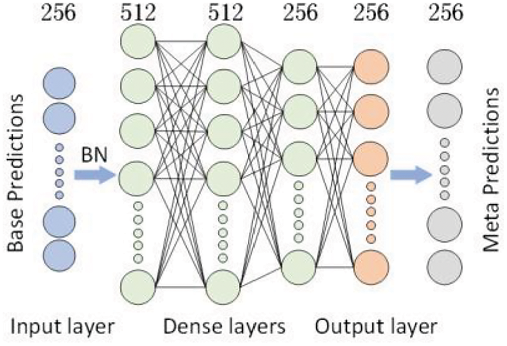
Figure 4: The MLP architecture

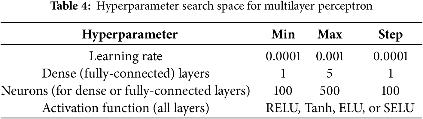
In Table 4, the range of MLP hyperparameters is indicated, which has a relatively limited number of combinations. It’s important to note that these ranges were selected as a rough estimate, aiming to achieve a good attack performance based on the results from related works. The architecture design of the MLP model is based on four hyperparameters. Network architectures with up to five fully connected layers are randomly selected. The number of neurons in each layer is chosen from the range {100, 200, 300, 400, 500}. Additionally, different activation functions are allowed to be searched, which can be randomly selected from {RELU, Tanh, ELU, SELU}. The Adam is used as the optimizer hyperparameter. The weight initialization uses the He uniform method, which mitigates the problem of gradient vanishing in deep networks and provides an effective starting point for model training.

4  Experimental Results

4.1 Comparison of Ensembles on Traditional Machine Learning and Deep Learning Models

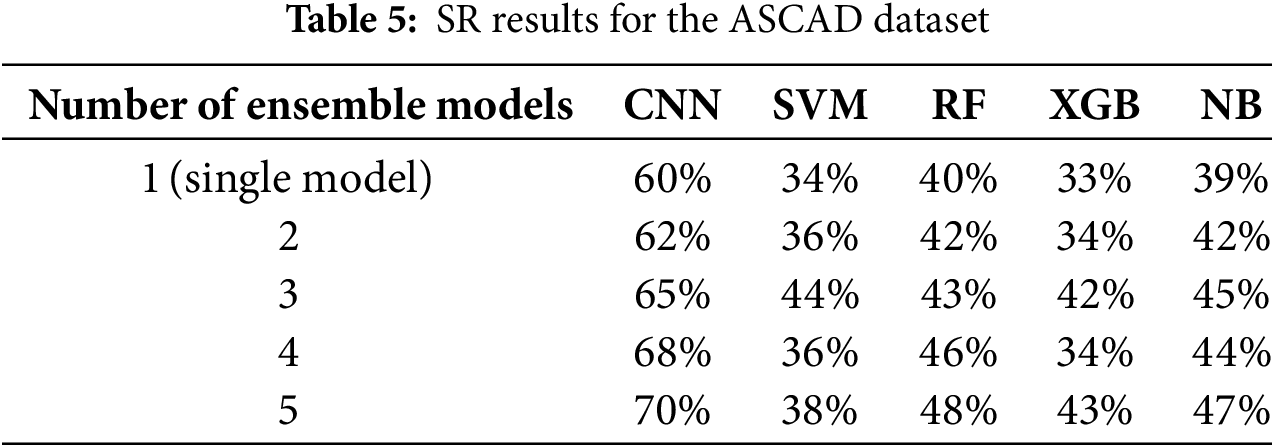
In this section, the performance of Stacking-SCA using traditional machine learning models and deep learning models (CNN and MLP) is compared, and the accuracy of the recovery traces under different feature dimensions. To ensure fairness, the selection of the base models is changed, and the meta-model is fixed to a simple MLP architecture. Experiments are conducted on the ASCAD dataset, and the integration of up to five models is considered.

In Table 5, the accuracy results of all tested methods on the protected implementation dataset are summarized. The success rate is used as a commonly used metric in SCA, to evaluate model performance, where the SR is defined as the number of correctly classified traces divided by the total number of attack traces. The experimental results show that CNN can achieve a success rate of 1 with fewer traces, significantly outperforming other models. For machine learning models, SVM demonstrates more stable accuracy when integrating more models. XGB performs best when three models are integrated, while both SVM and RF show significant improvement with five integrated models. In contrast, CNN is particularly suitable for handling high-dimensional and nonlinear data, exhibiting superior performance in feature selection and classification. Notably, despite the increased complexity that comes with adding more ensemble models, CNN still achieves a success rate of over 65%.

4.2 Results of the Stacking-SCA Method on Publicly Available Datasets

This section provides the experimental results of the Stacking-SCA methodology. Three publicly available datasets are considered. In our experiment, only the ID leakage model is considered to avoid the impact of data imbalance. For all experimental datasets, the attack is performed on a single key byte to calculate the GE. Additionally, experiments are conducted using ensembles of five and ten models, along with a single best model, and perform comparisons. Finally, the performance of our method is compared with other state-of-the-art works on the same datasets. Our experimental setup is deployed on a computer equipped with an NVIDIA GeForce GTX 3080Ti GPU. The deep learning models are implemented using Python3.8 version, with Tensorflow GPU 2.5 and Keras 2.5.1. To accommodate the requirements of the datasets, sufficient memory space is allocated for each task and the maximum virtual memory usage is increased to 50 GB.

4.2.1 ASCAD

The ASCAD dataset is divided into three subsets: 40,000 traces are used for training, 10,000 for testing, and 10,000 for attacking. Moreover, our learning rate is set to 5e-3, and the base model is trained for 50 epochs with a batch size of 50. The meta-model is trained for 10 epochs with a learning rate of 0.0001 and a batch size of 512.

To demonstrate the generalization capabilities of the ensemble approach, multiple hyper-parameter experimental designs are explored and the main internal structure is modified to consider the effects of multiple convolution kernels. As depicted in Fig. 5, representative ensembles of 3 models and 5 models are selected for attack testing. The hyperparameter settings for the convolution kernels are in the range of [1, 3], as most recent related works have used convolutional kernel parameters within this range. For most cases, these parameters show good convergence, with a single convolution kernel showing the best performance, successfully achieving key recovery only after about 200 traces.

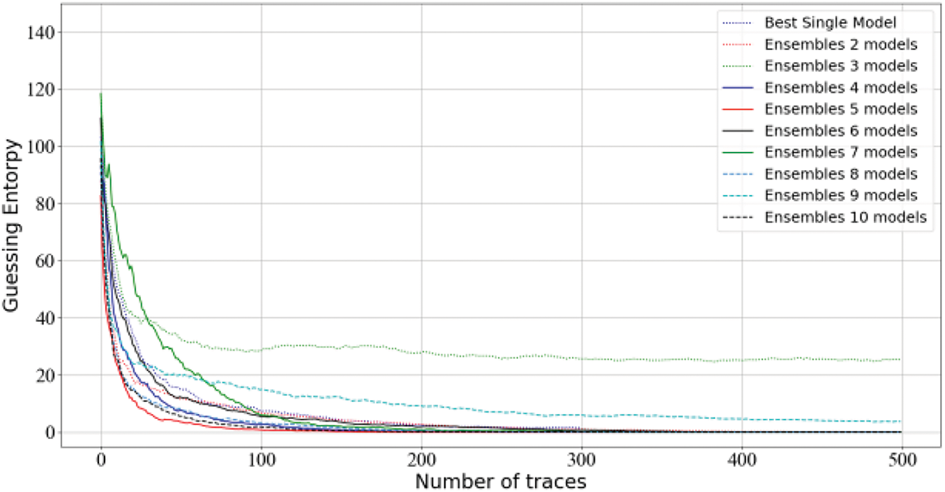
Figure 5: Ranking of CNN models using different convolution filter kernels with ensembles of 3 and 5 models on ASCAD

In Fig. 6, a comparison between ensembles ranging from two to ten models and the single best model is shown. The results show that Stacking-SCA achieves better performance when using an ensemble of five models, outperforming the single best model. However, as the number of ensemble models increases, the complexity also increases, impacting the training of the model. Specifically, for the ensemble of five models, the best performance reaches GE = 0 with approximately 160 traces. This difference becomes more pronounced as the number of traces increases in the training phase. For an ensemble of seven models, the performance shows a significant decline. Although increasing the number of base models can improve the attack performance, the results demonstrate that adding more models does not significantly improve generalization as expected. For an ensemble of three models, the model performance is unsatisfactory. It is speculated that the small number of ensembles may affect the overall effect, particularly when encountering more poorly performing models. Regarding the special performance of the ensemble of nine models, stable performance with a favorable trend is observed. Finally, our results are compared with Pieck et al. [31] who used the Bagging method on the ASCAD dataset. They chose to use between 10 and 50 models in the ensemble and select the best results among them. What is more, the Bagging method performs best with the ensemble of ten models, while keeping the original experimental settings. However, this approach requires 250 traces to reach a GE of 0 compared to our method. This result is not surprising, because Bagging typically considers the voting results of multiple models, and lacks the processing of data among the overall models.

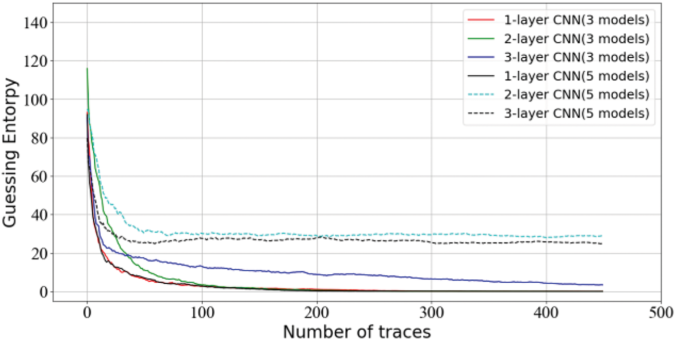
Figure 6: Guessing entropy results for Stacking-SCA on ASCAD

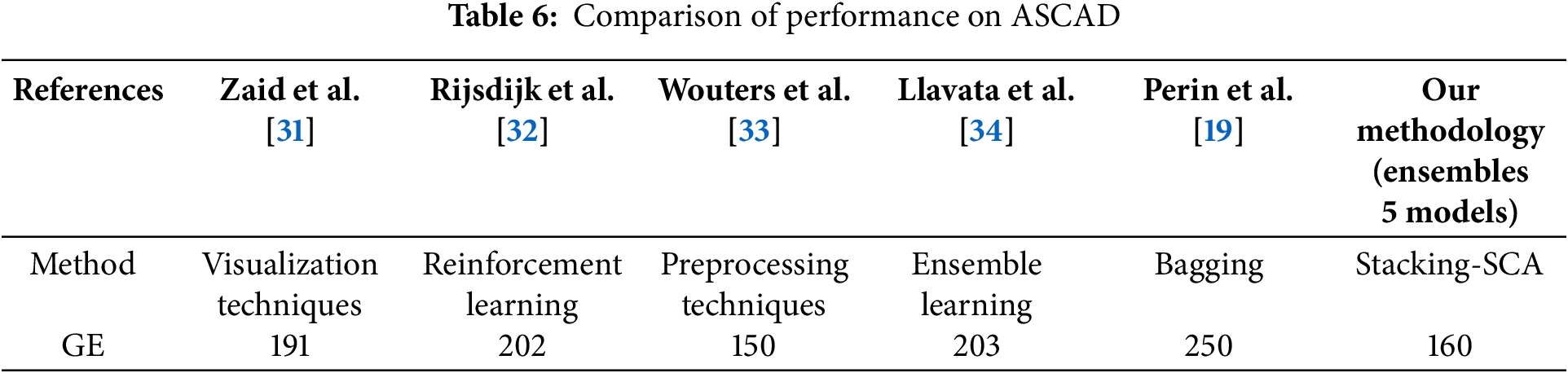
Next, in Table 6, a comparison is presented between our results in this paper and the results of state-of-the-art works. They are all experimented on the ID leakage model. Note that it is unfair to compare model training parameters with other architectures, because the number of trained models is already unequal. Zaid et al. [31] proposed a minimal CNN architecture, while in terms of performance, our method achieves better results. Rijsdijk et al. [32] employed reinforcement learning with a minimal reward function to reduce training parameters. Still, our performance difference with it is not so pronounced. Wouters et al. [33] optimized the internal structure, while our method achieved significantly better without optimizing the network size. It is believed that further enhancement of Stacking results could be achieved by considering more relevant expertise. The recent paper [34] investigates stacking on meta-model. Our approach differs by adjusting both the base models and the meta-model, and conducting a systematic analysis of the overall model performance.

4.2.2 DPAv4

The 5000 measurements are taken, with the training set containing 4000 traces, and the test and attack sets containing 500 traces each. Finally, 50 epochs are run for each base model with a learning rate of 1e-3, and a batch size of 512. For the meta-model, our learning rate is set to 0.0001. The training runs for 30 epochs with a batch size of 512. Fig. 7 shows another generalization case, where a three-layer CNN achieved the best prediction results. However, the performance of an ensemble of five models using only one convolution kernel exceeds our expectations, which may be related to the complexity of the convolutional layers.

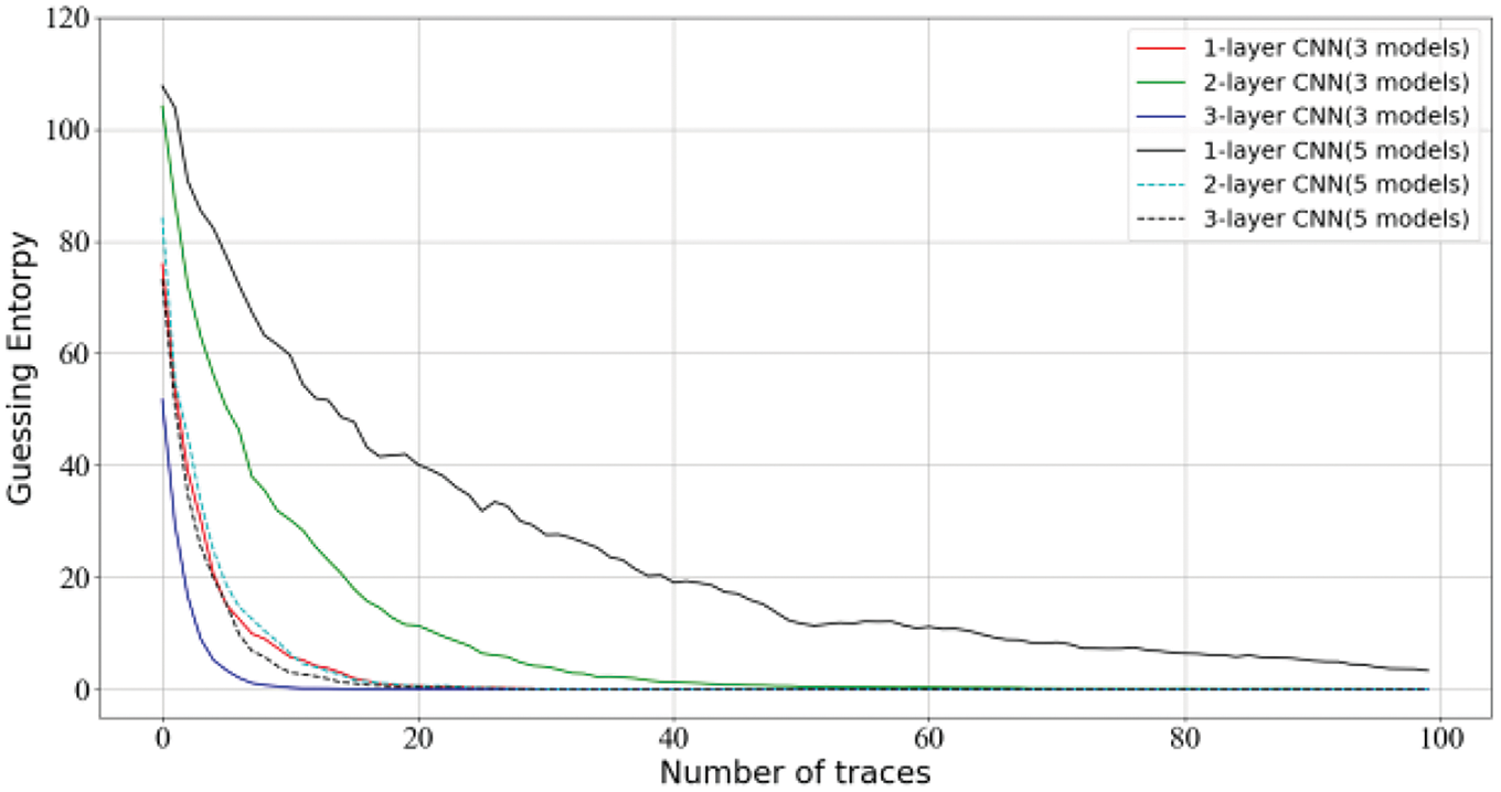
Figure 7: Ranking of CNN models using different convolution filter kernels with ensembles of 3 and 5 models on DPAv4

The results of our experiments are summarized in Fig. 8. The experimental results demonstrate that an ensemble of nine models achieves the best performance, requiring only three power traces to successfully recover the key. The overall attack performance is robust, effectively recovering the key with a minimal number of traces. Compared to the best single model experiment, the integration of multiple models converges significantly faster in terms of attack performance. Additionally, the difference between the ensemble of five and ten models is not particularly pronounced, which may be related to the complexity of the dataset. Next, the results of the Bagging method are presented on this dataset. Note that our dataset version differs from the one adopted by Pieck et al., as they used the DPAv4 subset with 2000 features in each trace. However, the performance of Bagging is significantly different from ours, as it requires 40 traces to reach GE of 0. This is mainly because the method is not very robust in combination with the models, and it is difficult to achieve good performance when the trained models have generalization problems.

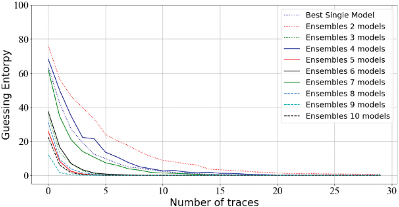
Figure 8: Guessing entropy results for Stacking-SCA on DPAv4

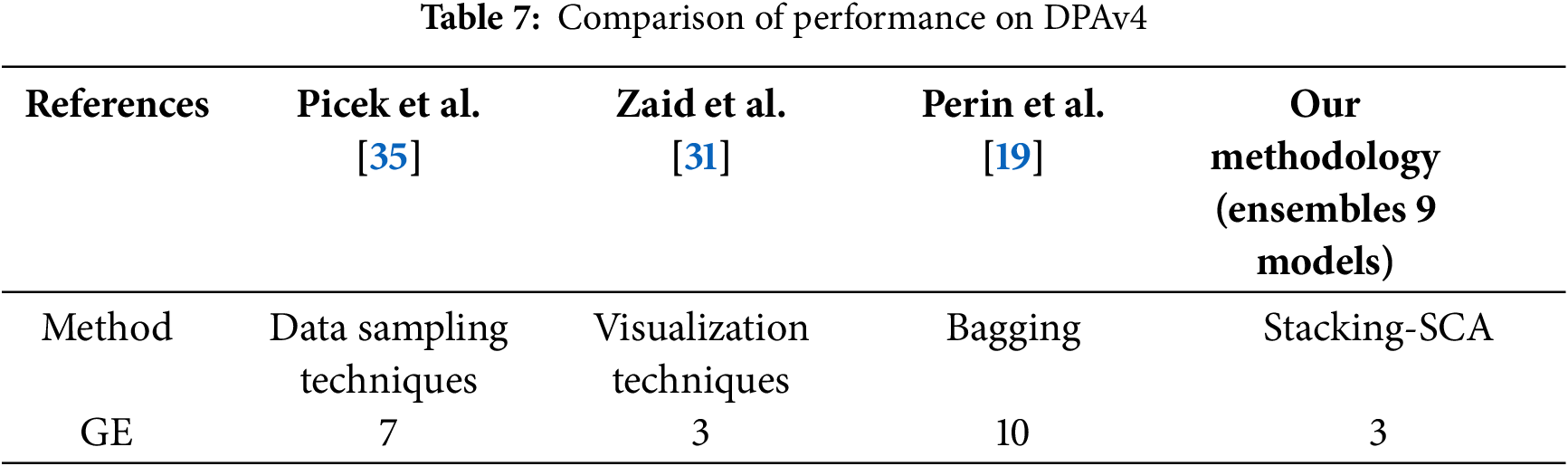
Table 7 shows the attack performance of some related results from state-of-the-art works. Our method reaches GE of 0 with fewer traces compared to several other architectures. Additionally, our method is compared with the machine learning techniques employed by Picek et al. [35], and noted that the performance related to deep learning techniques is more effective. Finally, Zaid et al. [31] achieved the optimal performance on this dataset at that time, which is comparable to our results.t be a new paragraph. Please punctuate equations as regular text.

4.2.3 AES_HD

Here, a total of 75,000 measurements are used, with 45,000 traces for training and 5000 traces for testing. Moreover, 25,000 traces are used for attacking. Then, the epoch of the base model is set to 20 with a batch size of 256, and a learning rate of 1e-3. As for the meta-model, our learning rate is set to 0.001. The training process is trained for 10 epochs with a batch size of 256. Fig. 9 indicates an example with relatively unclear convergence, where the key recovery is poorer when using three convolution kernels. Overall, the CNN with one convolution filter kernel size performs better, indicating that it has achieved better generalization ability.

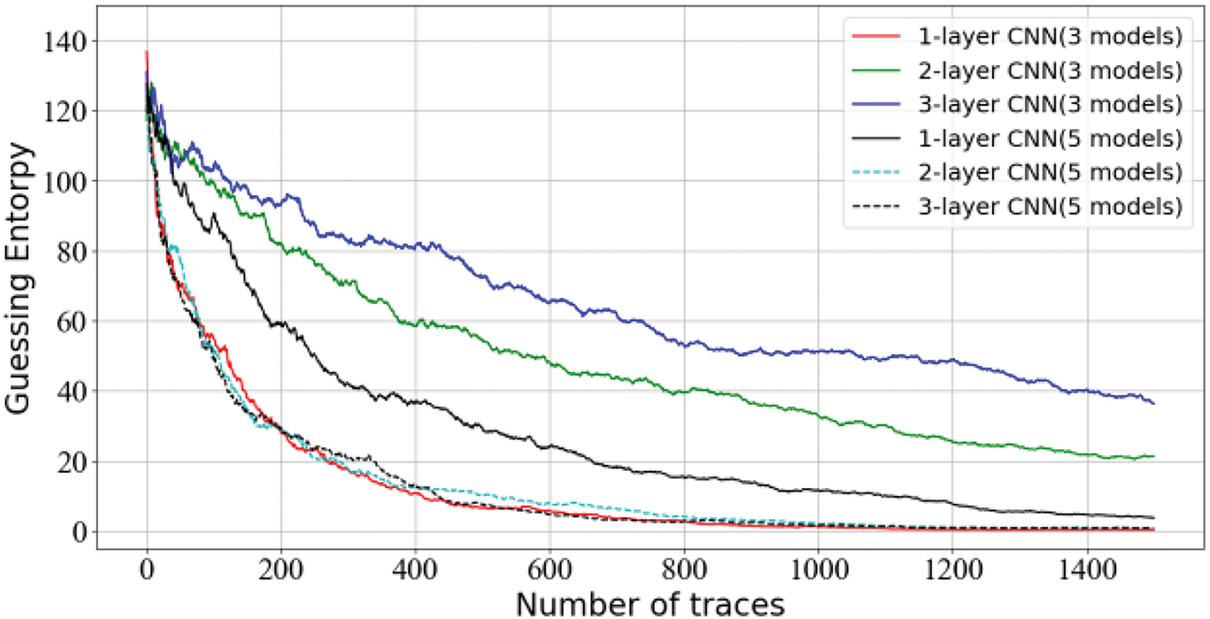
Figure 9: Ranking of CNN models using different convolution filter kernels with ensembles of 3 and 5 models on AES_HD

Fig. 10 shows the GE results for each ensemble on the AES_HD dataset. When integrating two models, the traces do not converge to GE = 0. Therefore, the number of models is increased, and some ensembles not only outperform the best single model but also the advantages between ensembles seem to be passed to each other. Interestingly, Stacking-SCA appears to effectively mitigate the impact of weaker models, demonstrating better robustness. When using an ensemble of eight models, it takes about 1000 traces to reach GE = 0. In contrast, other ensembles require more traces to achieve the same effect. This indicates that the ensemble of eight models reaches a local optimum, and further increasing the number of models may reduce the overall performance. Additionally, the experiments with the bagging method are not conducted on this dataset. Our analysis shows that the model performs poorly on this dataset, and attempts to train it do not yield satisfactory results.

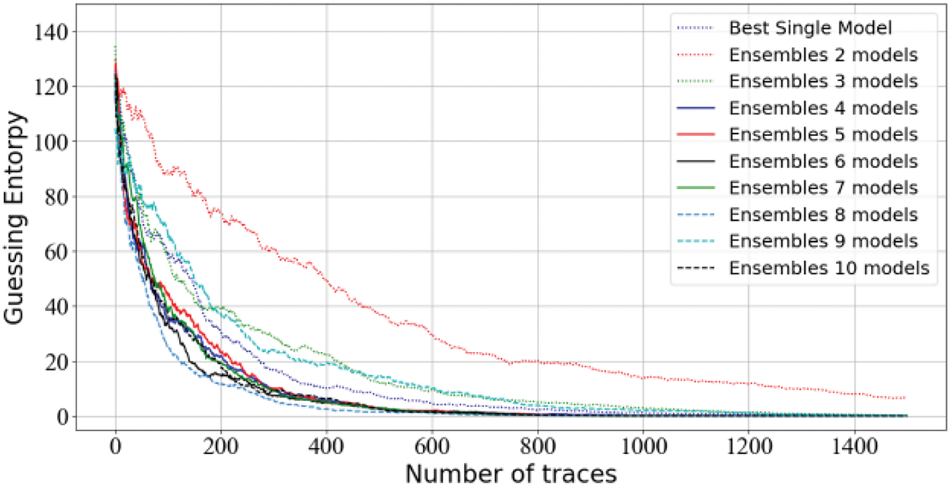
Figure 10: Guessing entropy results for Stacking-SCA on AES_HD

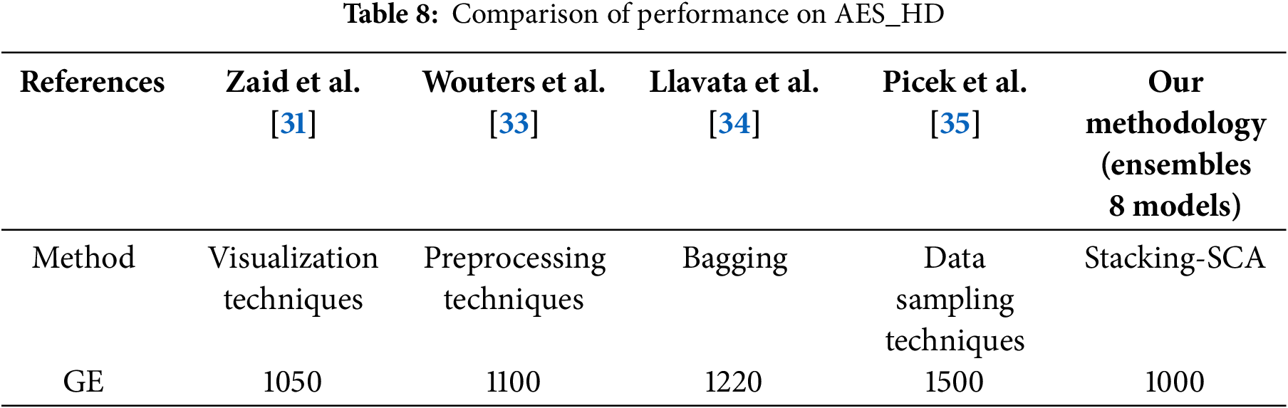
The comparison of attack performance improvements between our method and related works is summarized in Table 8. Note that the performance of Zaid et al. [31] is similar to our method, which requires 1050 traces to reach GE of 0. Compared to the method proposed by Llavata et al. in [34], our ensemble shows significantly better performance. Picek et al. [35] achieved good performance on this dataset using adversarial data imbalance techniques, but our method is significantly more efficient. The success of the ensemble not only relies on the meta-model but also requires the coordination of the overall model. Interestingly, our results perform better than Wouters et al. [33], in which they adjusted to the optimal model size, but the direct comparison with our ensemble differs significantly.

4.3 Results of the Stacking-SCA on the Multi-Segment Datasets

Following previous studies, in order to further understand the improvement of Stacking-SCA on model generalization, our experiments extend the application of this method to multi-segment datasets. Experiments are exclusively conducted on the ASCAD dataset, and results for the other two datasets are not provided. This is because the original ASCAD dataset has been extensively shared in the SCA community. It is difficult for us to assess the performance of other datasets in our experiments, although they may have similarities in certain aspects.

The five subsets are taken as inputs for Stacking-SCA, and divide each subset into three subsets: 40,000 traces are used for training, 10,000 for testing, and 10,000 for attacking. The base model is trained for 50 epochs, with a learning rate of 1e-3 and a batch size of 256. For the meta-model, 10 epochs are conducted, with a learning rate of 0.0001 and a batch size of 512. In Fig. 11, the GE results of the Stacking-SCA. Here, the experimental results show an enhancement in performance compared to the above results, it requires approximately 140 traces to reach GE of 0, which is 12% more efficient than the results on the ASCAD dataset.

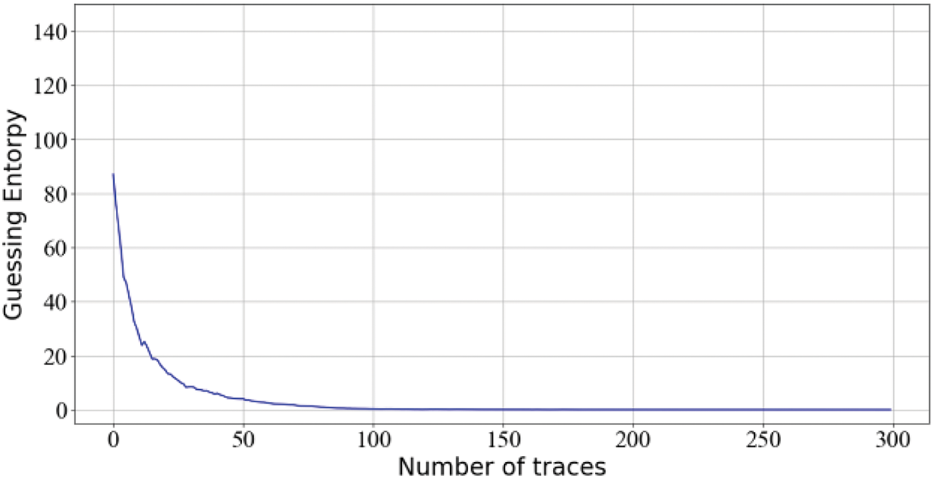
Figure 11: Guessing entropy results on the multi-segment datasets

5  Discussion

The Stacking-SCA method improves attack performance by integrating multiple models, which is usually accompanied by high computational overhead. In some resource-constrained environments, especially when performing real-time attacks on hardware platforms, the ensemble approach can lead to longer training times and increased computational burdens. Therefore, as the number of ensembles increases, the computational complexity also rises. To this end, it is recommended that a limited number of models, such as 10. This number is sufficient, as these integrated models are already quite complex and powerful, providing excellent attack performance. For DL-SCA, integrating multiple models is suggested as the standard for training, but the premise is to take into account resource consumption. This is especially important when dealing with high-dimensional datasets or limited hardware platforms, as the computational complexity of the Stacking-SCA may become a limiting factor.

Through experiments conducted on datasets extracted from hardware platforms such as ASCAD and AES_HD, this method performs excellently in real-world attack scenarios. Although the integration of multiple models is affected by the characteristics of the hardware platform (e.g., noise and countermeasures), the overall robustness remains strong. Interestingly, the ensemble model can achieve performance similar to that obtained through hyperparameter tuning, reducing the effort required for model tuning. This is closely related to the number of models in the ensemble and the impact of the maximum output class probability. However, ensemble methods also have certain limitations. Since stacking relies on the meta-model for the final prediction, overfitting can occur when there is insufficient training data, thereby affecting generalization. Therefore, it is necessary to find a suitable balance between the training trace and the number of models.

6  Conclusions and Future Works

This paper proposes a stacking ensemble method called Stacking-SCA. First, the method extends the overall model within the stacking framework and combines deep learning models to build base models and the meta-model, thereby improving the model’s output class probability. Experimental results show that the attack performance is significantly improved within a certain range of the number of models. Next, the input process of the method is optimized, leading to better generalization performance. Experiments on multiple publicly available datasets, demonstrate that when a certain number of models are integrated, the method shows good convergence. Compared to state-of-the-art results, the method shows a significant advantage in the GE indicator. This finding not only verifies the effectiveness of the Stacking-SCA method but also further highlights its potential in improving the performance of SCA. Therefore, the use of neural network integration is recommended as a priority in experiments, while also comprehensively considering the impact of model complexity.

In future work, there are some directions worth exploring in this promising field. The future scope of this work involves exploring the performance of the Stacking-SCA method across diverse hardware platforms, especially focusing on applications in low-power devices and IoT devices. Additionally, the potential advantages of ensemble learning in quantum attacks remain an unexplored area.

Acknowledgement: The authors also gratefully acknowledge the helpful comments and suggestions of the reviewers and editors, which have improved the presentation.

Funding Statement: This research is supported by the Hunan Provincial Natural Science Foundation of China (2022JJ30103), “the 14th Five-Year Plan” Key Disciplines and Application-Oriented Special Disciplines of Hunan Province (Xiangjiaotong [2022] 351), the Science and Technology Innovation Program of Hunan Province (2016TP1020).

Author Contributions: Zhicheng Yin, Lang Li: Conceptualization; Zhicheng Yin, Yu Ou: Methodology; Zhicheng Yin, Yu Ou: Writing—original draft preparation; Lang Li, Yu Ou: Writing—revision; Zhicheng Yin, Yu Ou: Experiment. All authors reviewed the results and approved the final version of the manuscript.

Availability of Data and Materials: There is no availability data and materials.

Ethics Approval: Not applicable.

Conflicts of Interest: The authors declare no conflicts of interest to report regarding the present study.

References

1. Ulitzsch VQ, Marzougui S, Tibouchi M, Seifert J. Profiling side-channel attacks on dilithium—A small bit-fiddling leak breaks it all. In: Selected Areas in Cryptography-29th International Conference, SAC 2022; Windsor, ON, Canada; 2022. Vol. 13742, p. 3–32. [Google Scholar]

2. Wu L, Perin G, Picek S. I choose you: automated hyperparameter tuning for deep learning-based side-channel analysis. IEEE Trans Emerg Top Comput. 2024;12(2):546–57. doi:10.1109/TETC.2022.3218372. [Google Scholar] [CrossRef]

3. Zhang C, Lu X, Cao P, Gu D, Guo Z, Xu S. A nonprofiled side-channel analysis based on variational lower bound related to mutual information. Sci China Inf Sci. 2023;66(1):100. doi:10.1007/s11432-021-3451-1. [Google Scholar] [CrossRef]

4. Timon B. Non-profiled deep learning-based side-channel attacks with sensitivity analysis. IACR Trans Cryptogr Hardw Embed Syst. 2019;2019:107–31. doi:10.46586/tches.v2019.i2.107-131. [Google Scholar] [CrossRef]

5. Zhou Z, Sun Y, Sun Q, Li C, Ren Z. Only once attack: fooling the tracker with adversarial template. IEEE Trans Circuits Syst Video Technol. 2023;33(7):3173–84. doi:10.1109/TCSVT.2023.3234266. [Google Scholar] [CrossRef]

6. Hu X, Meunier QL, Encrenaz E. Simple power analysis attacks using data with a single trace and no training. IACR Cryptol EPrint Arch. 2024;589(1):475–96. doi:10.46586/tches.v2025.i1.475-496. [Google Scholar] [CrossRef]

7. Go BS, Le DV, Song MG, Park M, Yu IK. Design and electromagnetic analysis of an induction-type coilgun system with a pulse power module. IEEE Trans Plasma Sci. 2018;47(1):971–6. doi:10.1109/TPS.2018.2874955. [Google Scholar] [CrossRef]

8. Lerman L, Bontempi G, Markowitch O. A machine learning approach against a masked AES: reaching the limit of side-channel attacks with a learning. J Cryptographic Eng. 2015;5(2):123–39. doi:10.1007/s13389-014-0089-3. [Google Scholar] [CrossRef]

9. Maghrebi H, Portigliatti T, Prouff E. Breaking cryptographic implementations using deep learning techniques. In: Security, Privacy, and Applied Cryptography Engineering: 6th International Conference, SPACE 2016,; 2016 Dec 14–18; Hyderabad, India. p. 3–26. [Google Scholar]

10. Mazhar T, Malik MA, Mohsan SAH, Li Y, Haq I, Ghorashi S, et al. Quality of service (QoS) performance analysis in a traffic engineering model for next-generation wireless sensor networks. Symmetry. 2023;15(2):513. doi:10.3390/sym15020513. [Google Scholar] [CrossRef]

11. Hajra S, Chowdhury S, Mukhopadhyay D. EstraNet: an efficient shift-invariant transformer network for side-channel analysis. IACR Trans Cryptogr Hardw Embed Syst. 2024;2024:336–74. [Google Scholar]

12. Hoang A, Hanley N, O’Neill M. Plaintext: a missing feature for enhancing the power of deep learning in side-channel analysis? breaking multiple layers of side-channel countermeasures. IACR Trans Cryptogr Hardw Embed Syst. 2020;2020:49–85. doi:10.46586/tches.v2020.i4.49-85. [Google Scholar] [CrossRef]

13. Wu L, Perin G, Picek S. The best of two worlds: deep learning-assisted template attack. IACR Trans Cryptogr Hardw Embed Syst. 2022;2022:413–37. doi:10.46586/tches.v2022.i3.413-437. [Google Scholar] [CrossRef]

14. Perin G, Wu L, Picek S. Exploring feature selection scenarios for deep learning-based side-channel analysis. IACR Trans Cryptogr Hardw Embed Syst. 2022;2022:828–61. doi:10.46586/tches.v2022.i4.828-861. [Google Scholar] [CrossRef]

15. Picek S, Perin G, Mariot L, Wu L, Batina L. SoK: deep learning-based physical side-channel analysis. ACM Comput Surv. 2023;55(11):1–35. doi:10.1145/3569577. [Google Scholar] [CrossRef]

16. Perin G, Buhan I, Picek S. Learning when to stop: a mutual information approach to prevent overfitting in profiled side-channel analysis. In: Constructive Side-Channel Analysis and Secure Design–12th International Workshop, COSADE 2021; Lugano, Switzerland; 2021. Vol. 12910, p. 53–81. [Google Scholar]

17. Zhang J, Zheng M, Nan J, Hu H, Yu N. A novel evaluation metric for deep learning-based side channel analysis and its extended application to imbalanced data. IACR Trans Cryptogr Hardw Embed Syst. 2020;2020:73–96. doi:10.46586/tches.v2020.i3.73-96. [Google Scholar] [CrossRef]

18. Lu X, Zhang C, Cao P, Gu D, Lu H. Pay attention to raw traces: a deep learning architecture for end-to-end profiling attacks. IACR Trans Cryptogr Hardw Embed Syst. 2021;2021:235–74. doi:10.46586/tches.v2021.i3.235-274. [Google Scholar] [CrossRef]

19. Perin G, Chmielewski L, Picek S. Strength in numbers: improving generalization with ensembles in machine learning-based profiled side-channel analysis. IACR Trans Cryptogr Hardw Embed Syst. 2020;2020:337–64. doi:10.46586/tches.v2020.i4.337-364. [Google Scholar] [CrossRef]

20. Hoang A, Hanley N, Khalid A, Kundi D, O’Neill M. Stacked ensemble models evaluation on DL based SCA. In: E-Business and Telecommunications–19th International Conference, ICSBT 2022; Lisbon, Portugal; 2022. Vol. 1849, p. 43–68. [Google Scholar]

21. Han S, Meng Z, Khan A, Tong Y. Incremental boosting convolutional neural network for facial action unit recognition. In: Advances in Neural Information Processing Systems 29: Annual Conference on NeuralInformation Processing Systems 2016; Barcelona, Spain; 2016. p. 109. [Google Scholar]

22. Cetiner M, Sahingoz OK. A comparative analysis for machine learning based software defect prediction systems. In: 11th International Conference on Computing, Communication and Networking Technologies, ICCCNT 2020; 2020 Jul 1–3. p. 1–7. [Google Scholar]

23. Wang K, Liu L, Yuan C, Wang Z. Software defect prediction model based on LASSO-SVM. Neural Comput Appl. 2021;33(14):8249–59. doi:10.1007/s00521-020-04960-1. [Google Scholar] [CrossRef]

24. Chen D, Zhang W, Xu X, Xing X. Deep networks with stochastic depth for acoustic modelling. In: Asia-Pacific Signal and Information Processing Association Annual Summit and Conference, APSIPA 2016; 2016 Dec 13–16. p. 1–4. [Google Scholar]

25. Ali M, Mazhar T, Arif Y, Al-Otaibi S, Ghadi YY, Shahzad T, et al. Software defect prediction using an intelligent ensemble-based model. IEEE Access. 2024;12(2):20376–95. doi:10.1109/ACCESS.2024.3358201. [Google Scholar] [CrossRef]

26. Mehta S, Patnaik KS. Improved prediction of software defects using ensemble machine learning techniques. Neural Comput Appl. 2021;33(16):10551–62. doi:10.1007/s00521-021-05811-3. [Google Scholar] [CrossRef]

27. Benadjila R, Prouff E, Strullu R, Cagli E, Dumas C. Deep learning for side-channel analysis and introduction to ASCAD database. J Cryptogr Eng. 2020;10(2):163–88. doi:10.1007/s13389-019-00220-8. [Google Scholar] [CrossRef]

28. González VZ, Tena-Sanchez E, Acosta AJ. A security comparison between AES-128 and AES-256 FPGA implementations against DPA attacks. In: 38th Conference on Design of Circuits and Integrated Systems, DCIS 2023; 2023 Nov 15–17. p. 1–6. [Google Scholar]

29. Hajra S, Saha S, Alam M, Mukhopadhyay D. Transnet: shift invariant trans-former network for side channel analysis. In: Progress in Cryptology–AFRICACRYPT 2022: 13th International Conference on Cryptology in Africa, AFRICACRYPT 2022; 2022. Vol. 13503, p. 371–96. [Google Scholar]

30. Ou Y, Li L, Li D, Zhang J. ESRM: an efficient regression model based on random kernels for side channel analysis. Int J Mach Learn Cybern. 2022;13(10):3199–209. doi:10.1007/s13042-022-01588-6. [Google Scholar] [CrossRef]

31. Zaid G, Bossuet L, Habrard A, Venelli A. Methodology for efficient CNN architectures in profiling attacks. IACR Transact Crypt Hardw Embed Syst. 2020;2020:1–36. doi:10.13154/tches.v2020.i1.1-36. [Google Scholar] [CrossRef]

32. Rijsdijk J, Wu L, Perin G, Picek S. Reinforcement learning for hyperparameter tuning in deep learning-basedside-channel analysis. IACR Trans Cryptogr Hardw Embed Syst. 2021;2021:677–707. doi:10.46586/tches.v2021.i3.677-707. [Google Scholar] [CrossRef]

33. Wouters L, Arribas V, Gierlichs B, Preneel B. Revisiting a methodology for efficient CNN architectures in profiling attacks. IACR Trans Cryptogr Hardw Embed Syst. 2020;2020(3):147–68. doi:10.13154/tches.v2020.i3.147-168. [Google Scholar] [CrossRef]

34. Llavata D, Cagli E, Eyraud R, Grosso V, Bossuet L. Deep stacking ensemble learning applied to profiling side-channel attacks. In: Smart Card Research and Advanced Applications–22nd International Conference, CARDIS 2023; Amsterdam, The Netherlands; 2023. Vol. 14530, p. 235–55. doi:10.1007/978-3-031-54409-5. [Google Scholar] [CrossRef]

35. Picek S, Heuser A, Jovic A, Bhasin S, Regazzoni F. The curse of class imbalance and conflicting metrics with machine learning for side-channel evaluations. IACR Trans Cryptogr Hardw Embed Syst. 2019;2019:209–37. doi:10.13154/tches.v2019.i1.209-237. [Google Scholar] [CrossRef]