A Method for Fast Feature Selection Utilizing Cross-Similarity within the Context of Fuzzy Relations

Abbreviations

1  Introduction

With the evolution of information technology, a substantial amount of information is captured in the form of data. These datasets contain a substantial quantity of redundant information. In data mining and model training, these redundant features can increase computational complexity and even result in model distortion, ultimately affecting the model’s predictive capability. Feature selection (or attribute selection, attribute reduction) is a crucial technique to minimize redundant features, aiming to identify the smallest subset of features that retain the distinguishability of the data.

Rough set theory [1] enjoys widespread application across diverse fields [2–4], with feature selection emerging as a particularly prominent research area within its scope. However, a limitation of rough set theory is its inability to handle continuous data directly. When dealing with features with continuous values, discretization is necessary, which can lead to the loss of valuable data information. To address these limitations of traditional rough set theory, Dubois et al. [5] introduced a novel concept by integrating fuzzy sets with rough sets, resulting in the emergence of a fuzzy rough set (FRS). This extension of Pawlak’s rough set model to the fuzzy domain represents a significant advancement in the field. Since then, researchers have conducted thorough investigations into fuzzy rough set theory, further refining its theoretical framework, alleviating constraints in practical applications, mitigating the impact of noisy data, and enhancing its overall robustness. Some researchers [6,7] have endeavored to generalize the fuzzy relationships among samples in fuzzy rough sets, broadening their scope and enhancing the model’s adaptability. Additionally, they have gone beyond the traditional definitions of the upper and lower approximation operators, giving the model a more comprehensive and flexible framework. These innovative extensions not only increase the model’s flexibility but also enable it to handle a wider range of practical applications with greater precision and adaptability. Despite the efforts of some researchers [8–11] to design more reasonable relationships and upper-lower approximation operations in order to mitigate the impact of noisy data and enhance the robustness of these fuzzy rough set models, they are often accompanied by increased computational complexity. Some researchers [12–16] have broadened the concept of fuzzy partition to fuzzy covering, thereby easing the constraints on the model’s application and enhancing its adaptability to diverse scenarios. This generalization not only facilitates a more flexible application of the model but also empowers it to tackle a broader spectrum of practical problems with enhanced precision and accuracy.

With the evolution of fuzzy rough set theory, numerous feature selection algorithms have emerged, built upon this theory. These algorithms aim to identify and extract salient features from datasets, aiding in their effective representation and interpretation. Jensen et al. [17] introduced the concepts of the fuzzy positive region and the fuzzy-rough dependency function, subsequently developing a feature selection model based on this dependency. Yang et al. [18] proposed a granular matrix and a granular reduction model, informed by fuzzy β-covering theory. Huang et al. [19,20] introduced a novel discernibility measure and a novel fitting model for attribute reduction, utilizing the fuzzy -neighborhood to capture the distinguishing power of a fuzzy covering family. Huang et al. [21] devised a robust rough set model that integrates fuzzy rough sets, covering-based rough sets, and multi-granulation rough sets. Furthermore, he successfully employed this model in the realm of feature selection. Wan et al. [22] proposed a novel interactive and complementary feature selection approach, which is based on the fuzzy multi-neighborhood rough set model, specifically designed for use with fuzzy and uncertain data. Hu et al. [23] developed a fuzzy multi-objective feature selection method, incorporating a fuzzy dominance relationship and particle swarm optimization. Deng et al. [24] formulated the dual similarity by leveraging the concept of neighborhood fuzzy entropy, and subsequently utilized it for feature selection in label distribution learning. Dai et al. [25] introduced the concept of multi-fuzzy -covering approximation spaces and subsequently proposed a forward greedy fuzzy -covering reduction algorithm, which is based on the monotone conditional entropy in a multi-fuzzy -covering approximation space.

Current feature selection algorithms predominantly employ forward greedy feature selection, that follows a sequential process, consisting of several distinct steps:

1)   Determine an evaluation metric.

2)   Model initialization: commences with an empty set as the selected feature subset and a candidate feature subset consisting of all features.

3)   Feature selection: in each iteration, incorporate one feature from the candidate feature subset to the already selected feature subset according to the evaluation metric. This process continues until the stopping criteria are satisfied.

When dealing with a dataset containing features and samples, the forward greedy feature selection algorithm, in the worst-case scenario, necessitates the calculation of the evaluation metric times. Moreover, for each evaluation of the evaluation metric, the calculation of relationships between every pair of samples in the dataset is essential, which necessitates calculating relationships between samples, such as distances or similarities. Consequently, the time complexity of these algorithms typically lies in the order of or higher. A significant challenge faced by these feature selection algorithms is their high computational complexity, which makes it challenging for them to effectively handle large sample sizes or high-dimensional data in practical settings.

Through rigorous research and meticulous analysis, we have identified the following issues with existing uncertainty measures and their corresponding feature selection algorithms:

1)   Existing feature selection algorithms must consider the relationships between all samples when calculating uncertainty measures (based on dependency or conditional information entropy).

2)   Existing sample relationships may exhibit weak associations due to noisy data, which can result in the selection of redundant features.

3)   Existing feature selection algorithms struggle to process large sample sizes or high-dimensional datasets effectively due to their high computational complexity.

Drawing upon the insights obtained, we introduce a novel and efficient feature selection algorithm that is grounded in cross-similarity. This algorithm represents a significant advancement in addressing the above challenges associated with feature selection. The primary contributions of this paper are outlined as follows:

1)   We establish a fuzzy binary relation known as the “cross-similarity relation”, which is highly sensitive to samples and relationships that impact the uncertainty of the decision tables while ignoring samples that are already consistent in the decision table.

2)   Using the cross-similarity relation as the uncertainty measure, we propose a new feature selection algorithm. Compared to existing feature selection algorithms, our algorithm reduces the time complexity from to .

3)   To mitigate the impact of noise-induced weak relationships, we introduce a truncation parameter that effectively reduces the influence of noisy data on the feature selection algorithm.

The paper is organized as follows: Section 2 covers the basics of similar relations and fuzzy rough sets. Section 3 introduces cross-similarity relations and their significance, along with their key properties. Section 4 details our new forward greedy feature selection model using fuzzy cross-similarity for data analysis. Section 5 presents experiments proving our method’s effectiveness, stability, and efficiency. Finally, Section 6 summarizes our findings, limitations of the algorithm, and further research directions.

2  Preliminaries

In this section, we will delve into the fundamental concepts of similar relations and fuzzy rough sets.

2.1 Similar Relations

In an information table, a binary relation among samples can be constructed based on the feature set. This binary relation is generally either a similarity relation [5,20,25] or a distance relation [7,26].

Definition 1. Let be a set of samples, be a set of conditional features, and be a set of similar relations between samples, where is a fuzzy compatible relation derived from the corresponding feature , signifying that and fulfills the properties of reflexivity and symmetry. Then, the pair is referred to as a fuzzy compatible relation space (FCRS).

Definition 2. Let be an FCRS, , and . Then is called a multi-attribute fuzzy compatible relation concerning .

Definition 3. A parameterized multi-attribute fuzzy compatible relation is defined as follows:

(1)

where .

The truncation parameter can be used to eliminate weak similarity relationships introduced by noisy data in the dataset. is capable of filtering out weak similarity relationships that exert influence on data uncertainty.

Proposition 4. Let be an FCRS. It holds that, for any ,

1)   if , then ;

2)   if then .

Proof. 1) For any , , .

2) If , then ; if , ; if , then . In summary, . □

2.2 Fuzzy Rough Sets

Definition 5. Let be an FCRS, with serving as the decision feature. Then the triple is known as a fuzzy decision table (FDT).

Let denote the ensemble of equivalent classes that are categorized by . can also be conceptualized as a fuzzy set, characterized by clear boundaries.

(2)

Definition 6. Let be an FCRS, , , and . Then the lower and upper approximations of concerning and are respectively as follows:

(3)

(4)

Then the quadruple () is called a fuzzy rough set model (FRSM) concerning and .

Proposition 7. Let () be an FRSM. Then the following conclusions hold:

1)   if , then ;

2)   if , then .

Proof. 1) Base on Proposition 4, for any , if , then .

2) Base on Proposition 4, for any , if , then . □

Proposition 8. Let () be an FRSM. Then the following conclusions hold:

1)   if , then ;

2)   if , then .

Proof of Proposition 8 follows a similar approach to Proposition 7.

Proposition 9. Let () be an FRSM. Then .

Proof. Based on Definitions 2.2 and 2.7, for any , , and , , so we have . □

Definition 10. Let be an FDT, and . If (), is referred to as a consistent sample regarding and . If all samples of demonstrate consistency, the FDT is considered a consistent one.

Proposition 11. Let be an , , , and . Then the following conclusions are true:

1)   if , then the sample is a consistent sample;

2)   if such that , then the sample x is an inconsistent sample.

Proof. 1) For , . For ; for . holds. , and , so .

For , , and , so ; . For ; and for holds. .

Hence, the sample is a consistent sample.

2) For , and , ; and , .

For , and , ; .

Hence, the sample is an inconsistent sample. □

3  Cross-Similarity

According to Proposition 11, the non-zero similarity of samples that are inconsistent originates from distinct classes. Hence, the focus should be exclusively on the similarity relationships that exist between samples belonging to different classes. Now, it’s time to delve into the intriguing concept of cross-similarity.

Definition 12. Let be an FDT, , , , and . The cross-similarity between and is defined as follows:

(5)

One can consider the FDT as a graph.

•   The samples in are visualized as nodes in the graph.

•   The parameterized multi-attribute similarity relations, designated as , are conceptually understood as undirected weighted edges connecting nodes within the graph. If , then there is no edge connecting node and node in the graph.

•   The equivalence relations derived from can be visualized as distinct enclosed areas within the graph.

By Definition 12, we narrow our focus to the similarity relations among samples belonging to distinct target partitions. The term “cross” denotes the intersection of the edge connecting samples of different target partitions and the boundary of enclosed areas, from a graphical perspective.

Definition 13. Let be an FDT, , , and . The fuzzy set with respect to is defined as follows:

(6)

The fuzzy set can be conceptualized as the fuzzy information granule of , with its cardinality represented as follows:

(7)

Let

and

(8)

represents the cross-similarity level of .

Proposition 14. Let be an FDT, , , and . The following conclusions are true:

1)   ;

2)   ;

3)   ;

4)   ;

5)   .

Proof. 1) By Definition 12, it is evident that

2) Under Definitions 2.2–2.4 and Definition 12, it is evident that this conclusion holds true;

3) According to 1), 2), and Eq. (8), it is evident that this conclusion holds true;

4) Since and , this conclusion is true;

5) In accordance with 3) and 4), and . □

Theorem 15. Let be an FDT, , , and . The following conclusions hold true:

1)   if , then ;

2)   if then .

Proof. 1) In accordance with Definition 12 and Proposition 4, it is evident that this conclusion holds true.

2) According to Definition 12 and Proposition 4, it is straightforward. □

Theorem 16. Let be an FDT, , and . The following conclusions hold true:

1)   if , then ;

2)   if then .

Proof. According to Theorem 15 and Eq. (7), it is straightforward to demonstrate the validity of these conclusions. □

Theorem 17. Let be an FDT, , and . The following conclusions are true:

1)   if , then ;

2)   if , then .

Proof. According to Theorem 16 Proposition 14, and Eq. (8), it is straightforward to demonstrate the validity of these conclusions. □

Example 1. Let be an , where and . is shown in Table 1, where and .

Target partition can be represented as a fuzzy set . The lower and upper approximations of under FCRS and parament are:

, .

Obviously, , there is uncertainty in the FCRS for Target partition . For a decision table, if there is an approximate inequality between the upper and lower parts of a decision partition, it is claimed that the decision table has uncertainty.

By Definition 13, the fuzzy set associated with each sample point is computed as follows:

Therefore, based on Definition 12, the FDT under and can be represented in Fig. 1. Each sample is represented as a node, a similarity relationship greater than 0 corresponds to an edge, and a target partition is depicted as an area enclosed by a dashed line in the graph. Cross-similarity relationships within similar relationships are highlighted in bold red.

Figure 1: Graphical representation of the FDT

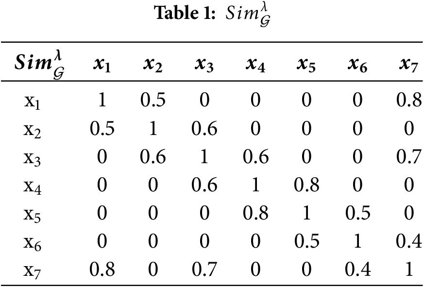
The cross-similarity matrix of the FDT is shown as follows:

Therefore, the cross-similarity level of is:

Theorem 18. Let be an FDT, and . If , the FDT is consistent:

Proof. , . Therefore, the FDT is consistent according to Proposition 11 1). □

Theorem 19. Let be an FDT, and . If , the FDT is inconsistent.

Proof. , , and . Therefore, the FDT is inconsistent according to Proposition 11 2). □

4  Feature Selection Based on Cross-Similarity

As decreases, the similarity between samples belonging to different classes diminishes. In other words, a low suggests that exhibits strong discriminatory capabilities. Consequently, serves as an effective tool for measuring the uncertainty associated with the FDT. The framework diagram of feature selection based on cross-similarity is shown in Fig. 2.

Figure 2: A framework diagram of feature selection

Definition 20. Let be an FDT, and . The is referred to as a reduction of , if

1)   ;

2)   .

Definition 21. Let be an FDT, , and . The significance of with respect to is defined as follows:

(9)

The larger is, the smaller becomes, making the more signicant.

Algorithm 1, a cross-similarity based feature selection (CSFS) algorithm, is a forward greedy feature selection algorithm.

Considering that as more features are chosen, the number of relationships to be considered when calculating cross-similarity progressively diminishes, and only the relationships between samples located in different categories are considered, the number of samples gradually decreases. It can be assumed that the number of samples decreases in geometric progression with a common ratio of . Then . Therefore, the time complexity of Algorithm 1 is improved to . In contrast, the time complexity of the feature selection algorithm based on positive domain, dependency, and conditional entropy is .

Example 2. A decision information table is shown in Table 2, where , and . Let and .

In this paper, the value of is determined through the utilization of the following equation:

(10)

where is the standard deviation of the attribute . By calculations, it is determined that , Let . Then , and are shown in Table 3.

The samples correspond to the nodes, similarity relations correspond to edges, bold red edges highlight the cross-similarity relations, and an area enclosed by a dashed line represents the target partition. The cross-similarity relation derived from is shown in Fig. 3.

Figure 3: Cross-similarity graph representation

Similarly, , and can be determined, as shown in Table 4.

If , let . Therefore, . If , let . .

According to Tables 3 and 4, we obtain , , and . Therefore, the minimum value is and . Thus, , and . Subsequently, we can obtain the following values by calculation. , and . Therefore, the minimum value is and . Thus, , and . Proceeding further, we have and . Therefore, the minimum value is and . Thus, , and . As , the feature selection process is terminated. As a result, the final feature selection outcome is . Given , and . Then, the descending sequence of sample sizes fulfills the condition:

5  Experimental Analysis

To establish the validity of CSFS, we conduct rigorous experimental comparisons between CSFS and five other state-of-the-art feature selection algorithms.

The following provides brief introductions to the five comparison algorithms, highlighting their key features and characteristics:

•   FRFS [15] (2024): It is a classic feature selection algorithm based on the dependency between the decision attribute and the conditional attributes subset.

•   FBC [18] (2020): It proposes a forward attribute selection algorithm based on conditional discernibility measure which can reflect the change of distinguishing ability caused by different attribute subsets.

•   NEFE [22] (2023): It provides a feature selection algorithm for label distribution using dual-similarity-based neighborhood fuzzy entropy.

•   MFBC [23] (2021): It is a feature selection algorithm based on the conditional information entropy under multi-fuzzy β-covering approximation space.

•   HANDI [24] (2022): It proposes a feature selection algorithm based on a neighborhood discrimination index, which can characterize the distinguishing information of a neighborhood relation.

5.1 Experimental Design

5.1.1 Evaluation Criteria

In the following three dimensions, we comprehensively evaluate the six algorithms, emphasizing their individual strengths and limitations.

•   The size of the selected feature subset.

•   The time cost of the feature selection process.

•   The performance of the selected feature subset in classification.

5.1.2 Classifiers

To conduct a rigorous and comprehensive evaluation of the efficacy of these six algorithms, we have chosen KNN (k = 5), SVM, and DT (CART) as the primary classification algorithms for assessing their classification accuracy. All other parameters of the three classifiers are set to default values. All testing procedures are conducted using ten-fold cross-validation for rigorous evaluation.

5.1.3 Experimental Environment

All experiments are implemented by Python 3.8.16 and scikit-learn 1.3.2, and run on a computer with an Intel(R) Xeon(R) Gold 5318Y CPU at 2.1 GHz, 128 GB RAM, and the operation system is Ubuntu18.04.1 LTS.

5.1.4 Datasets

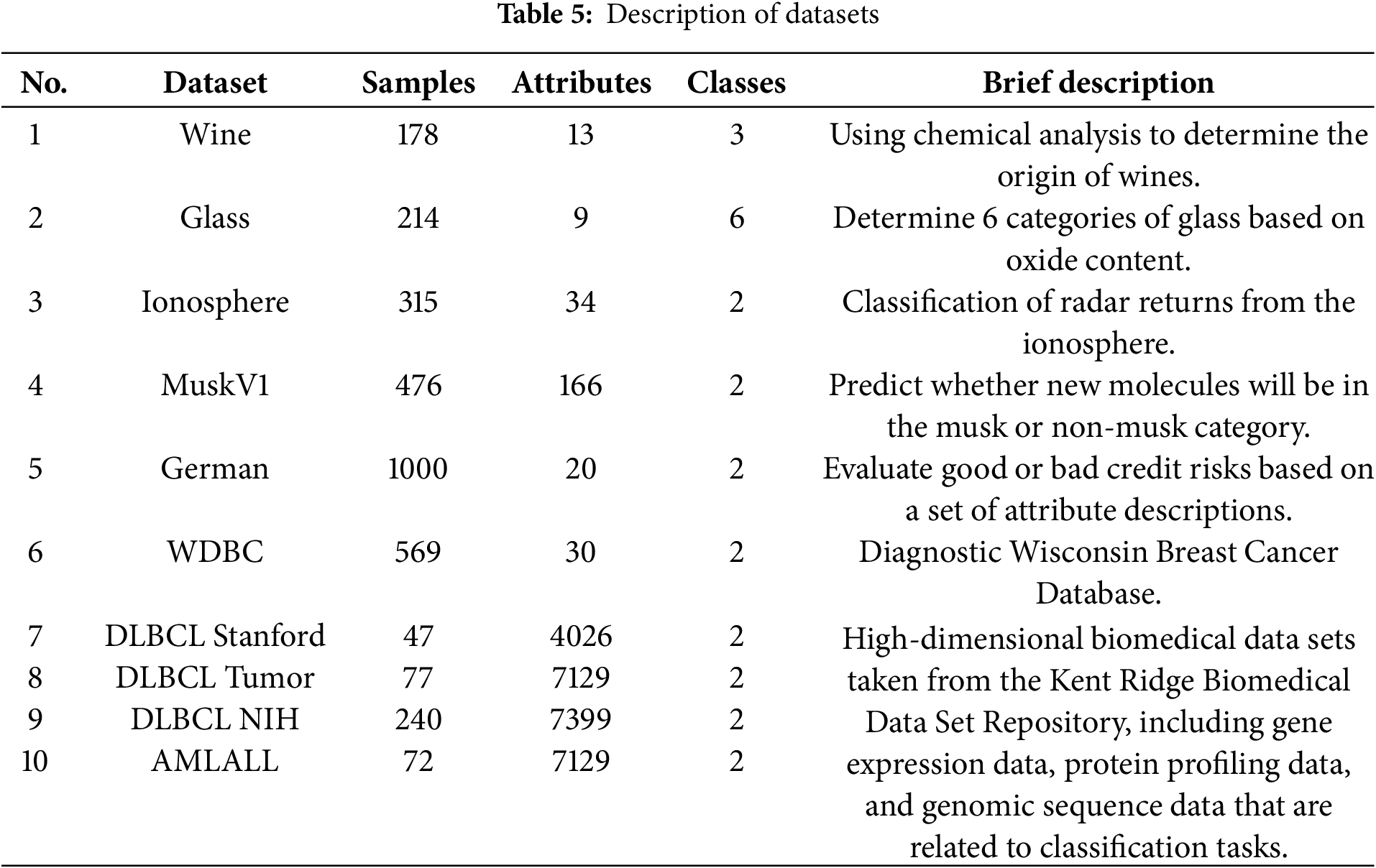
In our experiments, we utilized 10 publicly available datasets as benchmarks to assess the performance of various algorithms. The first six datasets, being of low dimension, were procured from the UCI Machine Learning Repository [27], whereas the remaining four high-dimensional datasets were retrieved from the KRBD Repository [28]. For a comprehensive overview of these datasets, please refer to Table 5, which provides detailed descriptions of each dataset’s characteristics. If there are missing values in the dataset, we will fill them with the average value of samples that belong to the same class and have the same feature as the missing value.

5.1.5 Parameter Settings

Among the six algorithms, FRFS stands alone as the sole algorithm that does not involve any parameters. To ensure the fairness and integrity of comparative experiments, we employ a meticulous grid search approach to identify the optimal parameter values for all algorithms encompassing parameters. The step size of the CSFS algorithm has been set to 0.01, while the step sizes of other algorithms have been configured to 0.1. As per the specifications provided in the respective references for each algorithm, the search scope of the parameters is summarized in Table 6. The reason why the other algorithms set the step size to 0.1 instead of 0.01 is that if they also set the step size to 0.01, the experiments would not be able to complete. Initially, we outline the time taken by each algorithm in their search for optimal parameters. Subsequently, we present the optimal parameter values that were chosen based on their classification accuracy.

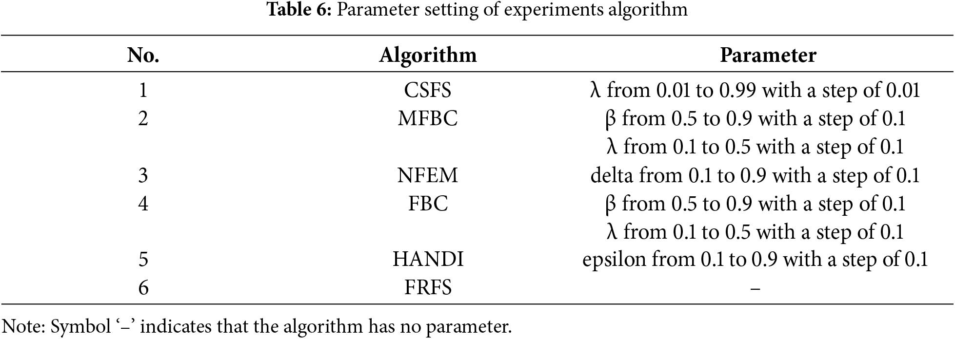
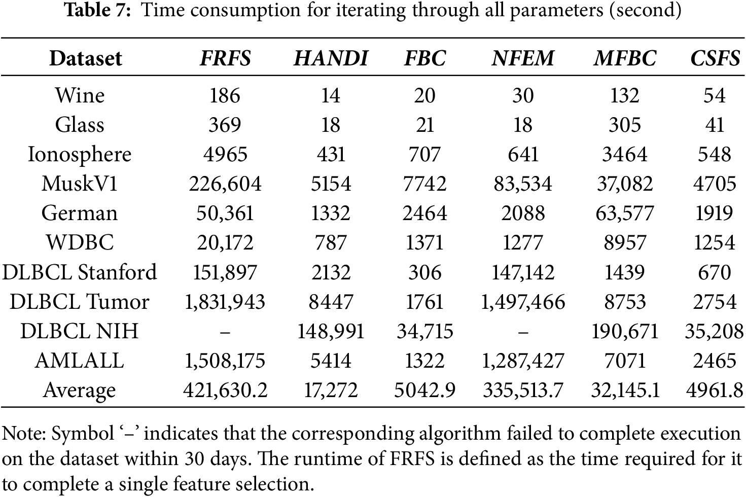
Table 7 provides an enumeration of the total time consumed by each algorithm on each dataset when running all possible parameters under the parameter configuration outlined in Table 7. Notably, CSFS stands out in terms of efficiency, consistently achieving the lowest average time for parameter search across all datasets.

5.2 Result Analysis

5.2.1 The Size of the Selected Feature Subset

Table 8 presents the count of features chosen by six feature selection algorithms across ten datasets. FRFS and NFEM were terminated early due to excessive runtime, hence their outcomes are undisclosed.

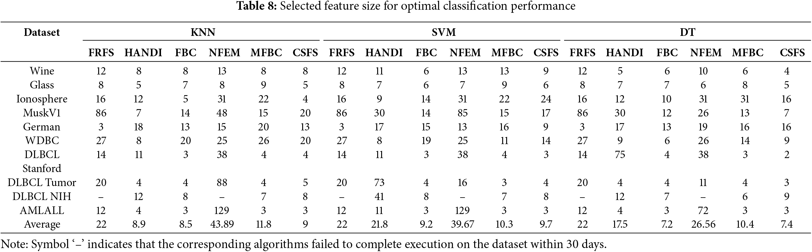
Table 8 indicates the following findings:

•   In comparison to the original feature count in Table 5, it is noteworthy that these feature selection algorithms effectively select salient features and reduce data redundancy.

•   The optimal feature subsets for different classifiers can vary.

•   CSFS selects fewer features than FRFS, HANDI, NFEM, and MFBC, yet slightly more than FBC.

5.2.2 The Runtime of the Algorithms

Table 9 and Fig. 4 present a comparison of the time taken by the six feature selection algorithms to execute a feature selection using parameters that achieved the highest classification accuracy for each classifier.

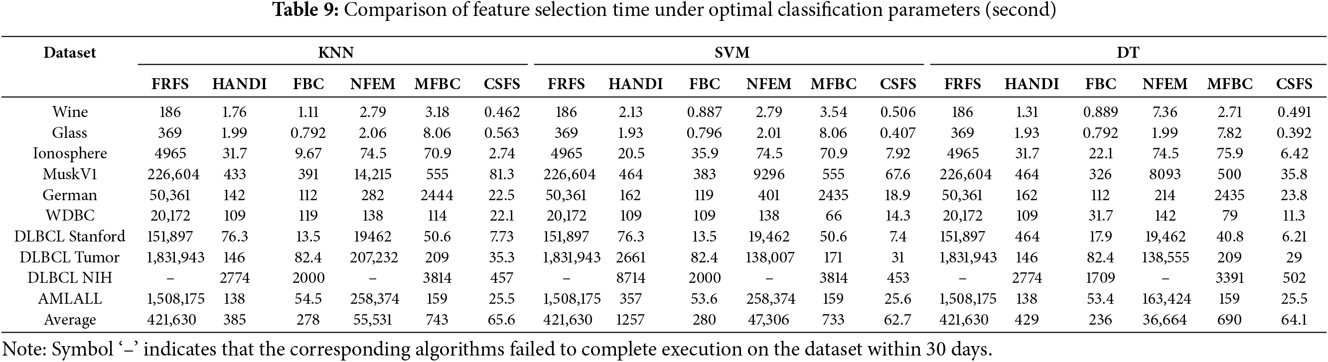
Figure 4: The time consumption of the feature selection process across various datasets. (a) KNN classifier with the optimal parameter. (b) SVM classifier with the optimal parameter. (c) DT classifier with the optimal parameter. FRFS and NFEM failed to complete execution on the DLBCLNIH dataset within 30 days and the runtime is set to 2,592,000 s (30 days)

Table 9 and Fig. 4a–c indicate the following findings:

•   When it comes to time efficiency, CSFS outperforms all other algorithms, exhibiting a clear advantage. The scale of the vertical axis representing time consumption in the graph is exponentially increasing.

•   As the sample size increases, the advantage of CSFS becomes increasingly apparent. This observation is consistent with the theoretical time complexity of CSFS, which is .

It is worth noting that for the DLBCL NIH dataset with 240 samples and 7399 conditional attributes, as the dimensionality increases, the time required for feature selection by the comparison algorithms is significantly higher than that of the CSFS algorithm. The NFEM algorithm is even unable to produce results within an acceptable time frame.

5.2.3 Classification Accuracy

Tables 10–12 present the classification accuracy of three distinct classifiers across the selected feature subsets of the six algorithms. The highest classification accuracy is boldly displayed.

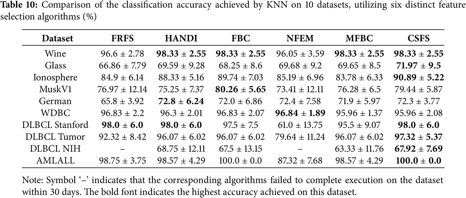
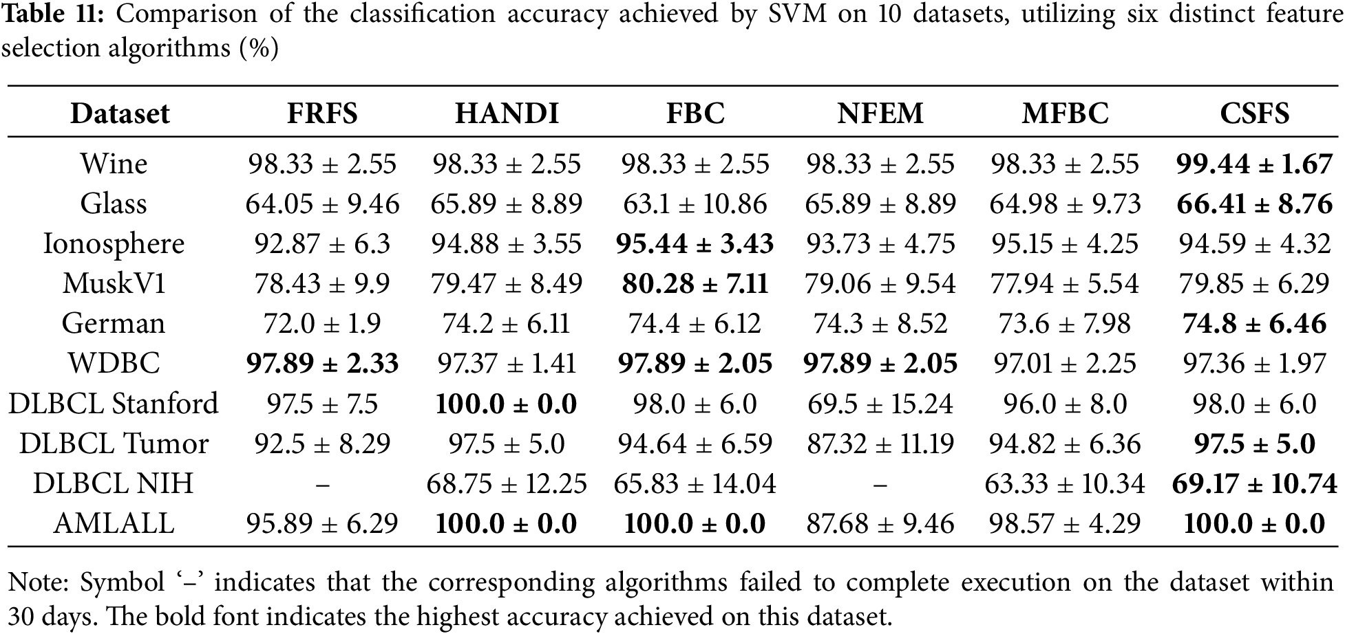
Tables 10–12 clearly indicate the following findings:

•   Through 30 rigorous evaluations, algorithm CSFS has emerged as the clear leader, achieving the highest classification accuracy on 19 occasions. In comparison, algorithm FBC excelled on 11 occasions, while algorithms HANDI and MFBC delivered the best results on 8 and 3 occasions, respectively. Algorithms FRFS and NFEM lagged behind, achieving the highest accuracy on just 2 occasions each.

•   The standard deviation values clearly indicate that the features selected by algorithm CSFS exhibit excellent representativeness, providing a stable and accurate representation of the data.

Compared with other comparison methods, the CSFS algorithm focuses more attention on samples that have not yet been perfectly partitioned under current conditions when measuring the uncertainty of target attributes in feature subsets and is more sensitive to improving the uncertainty of such samples when selecting subsequent features.

5.3 Parameter Analysis

The value of parameter ‘’ in the CSFS algorithm impacts the outcome of feature selection. In Fig. 5a–d, we can observe the correlation between the number of selected features and the value of parameter ‘’ in the CSFS algorithm. In Fig. 6a–d, we can observe the correlation between the classification accuracy of selected features and the value of parameter ‘’ in the CSFS algorithm.

Figure 5: The impact of parameter ‘’ on the number of selected features

Figure 6: The impact of parameter ‘’ on the classification accuracy of selected features. (a) DLBCL Stanford (b) DLBCL Tumor (c) DLBCL NIH (d) AMLALL

Figs. 5 and 6 clearly indicate the following findings:

•   As the value of parameter ‘’ increases, the overall tendency is for the number of selected features to decrease. This is because with an increase in the value of ‘’, the number of cross-similar relationships being removed also rises.

•   When the value of parameter ‘’ surpasses a certain threshold, the classification accuracy undergoes a drastic drop. This is because at high values of ‘’, crucial information is also being eliminated, leading to a significant decline in performance.

•   The parameter ‘’ serves to eliminate noisy and redundant relationships, hence the value of ‘’ should generally not be set too high.

Let’s illustrate the impact of the truncation parameter on noise reduction in feature selection through a specific case. For the gene dataset DLBCL NIH, which contains noisy data, by observing Fig. 6c, we find that as increases from a small value to a large one, the accuracy of the selected attribute subset in the classifier first increases and then decreases. This indicates that within a certain range, the parameter can effectively eliminate the impact of noise and identify a truly meaningful subset of attributes for target classification.

6  Conclusions and Discussions

In this article, we introduce a novel and unique metric for quantifying data uncertainty, termed cross-similarity. This metric iteratively emphasizes similarity relations that substantially influence the uncertainty of fuzzy decision tables. Leveraging this metric, we have devised a forward greedy feature selection algorithm, known as CSFS. The CSFS algorithm significantly reduces the time complexity of feature selection algorithms based on fuzzy rough sets, transforming it from O (m2n2) to O (mn2), thereby greatly enhancing computational efficiency. Experimental results validate that the CSFS algorithm not only accelerates the feature selection process but also accurately identifies the most representative features. Consequently, our algorithm effectively tackles the challenges posed by the high computational complexity of existing fuzzy rough set-based feature selection algorithms.

However, the CSFS algorithm also has some limitations. Firstly, when integrating multi-attribute similarity relationships, it relies on the minimum similarity relationship, making the algorithm sensitive to outlier features. Secondly, the uncertainty measure is based on cross-similarity within the decision table, thus its application is limited to comparing the uncertainty of different attribute subsets within the same decision table, rather than across different decision tables.

In response to the above limitations, our future research endeavors will encompass the following: Firstly, we aim to delve into multi-attribute similarity metrics that consider sample distribution or incorporate linear reconstruction of samples prior to similarity assessment. Both approaches hold promise in reducing the impact of outlier features, ultimately bolstering the algorithm’s robustness. Secondly, to navigate the trade-off between computational complexity and robustness, we will explore the potential of parallel computing. Lastly, we will undertake further research into normalized uncertainty measures grounded in cross-similarity, with the objective of expanding their applicability across diverse scenarios.

Acknowledgement: The authors would like to thank the anonymous reviewers for their valuable comments.

Funding Statement: This work was supported by the Anhui Provincial Department of Education University Research Project (2024AH051375), Research Project of Chizhou University (CZ2022ZRZ06), Anhui Province Natural Science Research Project of Colleges and Universities (2024AH051368) and Excellent Scientific Research and Innovation Team of Anhui Colleges (2022AH010098).

Author Contributions: The authors confirm their contribution to the paper as follows: study conception and design: Wenchang Yu; analysis and interpretation of results: Xiaoqin Ma, Zheqing Zhang; draft manuscript preparation: Qinli Zhang. All authors reviewed the results and approved the final version of the manuscript.

Availability of Data and Materials: Not applicable.

Ethics Approval: Not applicable.

Conflicts of Interest: The authors declare no conflicts of interest to report regarding the present study.

References

1. Pawlak Z. Rough sets. Int J Comput Inf Sci. 1982;11(4):341–56. doi:10.1007/BF01001956. [Google Scholar] [CrossRef]

2. Dinçer H, Yüksel S, An J, Mikhaylov A. Quantum and AI-based uncertainties for impact-relation map of multidimensional NFT investment decisions. Finance Res Lett. 2024;66(3):105723. doi:10.1016/j.frl.2024.105723. [Google Scholar] [CrossRef]

3. Kamran M, Salamat N, Jana C, Xin Q. Decision-making technique with neutrosophic Z-rough set approach for sustainable industry evaluation using sine trigonometric operators. Appl Soft Comput. 2025;169(2):112539. doi:10.1016/j.asoc.2024.112539. [Google Scholar] [CrossRef]

4. Banerjee M, Mitra S, Banka H. Evolutionary rough feature selection in gene expression data. IEEE Trans Syst Man Cybern C Appl Rev. 2007;37(4):622–32. doi:10.1109/TSMCC.2007.897498. [Google Scholar] [CrossRef]

5. Dubois D, Prade H. Rough fuzzy sets and fuzzy rough sets. Int J Gen Syst. 1990;17(3):191–209. doi:10.1080/03081079008935107. [Google Scholar] [CrossRef]

6. Mi J, Leung Y, Zhao H, Feng T. Generalized fuzzy rough sets determined by a triangular norm. Inf Sci. 2008;178(12):3203–13. doi:10.1016/j.ins.2008.03.013. [Google Scholar] [CrossRef]

7. Yao W, Zhang G, Zhou C. Real-valued hemimetric-based fuzzy rough sets and an application to contour extraction of digital surfaces. Fuzzy Sets Syst. 2023;459(1–3):201–19. doi:10.1016/j.fss.2022.07.010. [Google Scholar] [CrossRef]

8. Zhang QL, Chen YY, Zhang GQ, Li ZW, Chen LJ, Wen CF. New uncertainty measurement for categorical data based on fuzzy information structures: an application in attribute reduction. Inf Sci. 2021;580(5):541–77. doi:10.1016/j.ins.2021.08.089. [Google Scholar] [CrossRef]

9. Yao Y, Zhao Y. Attribute reduction in decision-theoretic rough set models. Inf Sci. 2008;178(17):3356–73. doi:10.1016/j.ins.2008.05.010. [Google Scholar] [CrossRef]

10. Zhao S, Tsang E, Chen D, Wang X. Building a rule-based classifier—a fuzzy-rough set approach. IEEE Trans Knowl Data Eng. 2009;22(4):624–38. doi:10.1109/TKDE.2009.118. [Google Scholar] [CrossRef]

11. Hu Q, Zhang L, An S, Zhang D, Yu D. On robust fuzzy rough set models. IEEE Trans Fuzzy Syst. 2011;20(4):636–51. doi:10.1109/TFUZZ.2011.2181180. [Google Scholar] [CrossRef]

12. Ma L. Two fuzzy covering rough set models and their generalizations over fuzzy lattices. Fuzzy Sets Syst. 2016;294(11):1–17. doi:10.1016/j.fss.2015.05.002. [Google Scholar] [CrossRef]

13. Deer L, Cornelis C. A comprehensive study of fuzzy covering-based rough set models: definitions, properties and interrelationships. Fuzzy Sets Syst. 2018;336(16):1–26. doi:10.1016/j.fss.2017.06.010. [Google Scholar] [CrossRef]

14. Yang B, Hu B. On some types of fuzzy covering-based rough sets. Fuzzy Sets Syst. 2017;312:36–65. doi:10.1016/j.fss.2016.10.009. [Google Scholar] [CrossRef]

15. Zhang Q, Yan S, Peng Y, Li Z. Attribute reduction algorithms with an anti-noise mechanism for hybrid data based on fuzzy evidence theory. Eng Appl Artif Intell. 2024;129:107659. doi:10.1016/j.engappai.2023.107659. [Google Scholar] [CrossRef]

16. Zhang L, Zhan J. Fuzzy soft β-covering based fuzzy rough sets and corresponding decision-making applications. Int J Mach Learn Cybern. 2019;10(6):1487–502. doi:10.1007/s13042-018-0828-3. [Google Scholar] [CrossRef]

17. Jensen R, Shen Q. Fuzzy-rough sets assisted attribute selection. IEEE Trans Fuzzy Syst. 2007;15(1):73–89. doi:10.1109/TFUZZ.2006.889761. [Google Scholar] [CrossRef]

18. Yang T, Zhong X, Lang G, Qian Y, Dai J. Granular matrix: a new approach for granular structure reduction and redundancy evaluation. IEEE Trans Fuzzy Syst. 2020;28(12):3133–44. doi:10.1109/TFUZZ.2020.2984198. [Google Scholar] [CrossRef]

19. Huang Z, Li J. A fitting model for attribute reduction with fuzzy XX-covering. Fuzzy Sets Syst. 2021;413:114–37. doi:10.1016/j.fss.2020.07.010. [Google Scholar] [CrossRef]

20. Huang Z, Li J. Discernibility measures for fuzzy β covering and their application. IEEE Trans Cybern. 2021;52(4):9722–35. doi:10.1109/TCYB.2021.3054742. [Google Scholar] [PubMed] [CrossRef]

21. Huang Z, Li J, Qian Y. Noise-tolerant fuzzy-β-covering-based multigranulation rough sets and feature subset selection. IEEE Trans Fuzzy Syst. 2021;30(9):2721–35. doi:10.1109/TFUZZ.2021.3093202. [Google Scholar] [CrossRef]

22. Wan J, Chen H, Li T, Yuan Z, Liu J, Huang W, et al. Interactive and complementary feature selection via fuzzy multigranularity uncertainty measures. IEEE Trans Cybern. 2023;53(2):1208–21. doi:10.1109/TCYB.2021.3112203. [Google Scholar] [PubMed] [CrossRef]

23. Hu Y, Zhang Y, Gong D. Multiobjective particle swarm optimization for feature selection with fuzzy cost. IEEE Trans Cybern. 2021;51(3):874–88. doi:10.1109/TCYB.2020.3015756. [Google Scholar] [PubMed] [CrossRef]

24. Deng Z, Li T, Deng D, Liu K, Zhang P, Zhang S, et al. Feature selection for label distribution learning using dual-similarity based neighborhood fuzzy entropy. Inf Sci. 2022;615(10):385–404. doi:10.1016/j.ins.2022.10.054. [Google Scholar] [CrossRef]

25. Dai J, Zou X, Qian Y, Wang X. Multifuzzy β-covering approximation spaces and their information measures. IEEE Trans Fuzzy Syst. 2022;31(5):955–69. doi:10.1109/TFUZZ.2022.3193448. [Google Scholar] [CrossRef]

26. Wang C, Hu Q, Wang X, Chen D, Qian Y, Dong Z. Feature selection based on neighborhood discrimination index. IEEE Trans Neural Netw Learn Syst. 2017;29(8):2986–99. doi:10.1109/TNNLS.2017.2710422. [Google Scholar] [PubMed] [CrossRef]

27. UCI machine learning repository [Internet]. Irvine, CA, USA: University of California; [cited 2024 Oct 1]. Available from: http://archive.ics.uci.edu. [Google Scholar]

28. Kent Ridge bio-medical data set repository [Internet]. Granada, Spain: University of Granada; [cited 2024 Oct 1]. Available from: https://leo.ugr.es/elvira/DBCRepository. [Google Scholar]