Semi-Supervised New Intention Discovery for Syntactic Elimination and Fusion in Elastic Neighborhoods

1  Introduction

Dialogue generation is a key research area in natural language processing [1], with intent recognition serving as its foundation. Accurate intent identification is essential for addressing dialogue generation challenges. However, existing models cannot directly recognize undefined intents, requiring unknown intents to be mapped to predefined categories. New intent discovery clusters similar unknown intents, facilitating intent definition and reducing the complexity of dialogue generation across various domains [2]. Leveraging labeled intent data for semi-supervised new intent discovery is crucial [3], as it improves unknown intent recognition and advances dialogue generation development [4].

Pre-trained models possess strong sentence representation capabilities. Bidirectional Encoder Representations from Transformers (BERT), proposed by Devlin et al. [5], laid the foundation for pre-trained models with its encoder-only architecture. It captures rich contextual information using the Masked Language Modeling (MLM) task and the Next Sentence Prediction (NSP) task. Building on BERT, Roberta, proposed by Liu [6], removes the NSP objective and optimizes hyperparameters. DistilBERT, introduced by Sanh [7] reduce the size of BERT using knowledge distillation techniques while retaining most of its performance, making it more efficient for real-time applications. ALBERT, proposed by Lan et al. [8], introduces parameter sharing and factorized embedding techniques, significantly reducing the model size while maintaining competitiveness in natural language understanding tasks. Efficiently Learning an Encoder that Classifies Token Replacements Accurately (ELECTRA), proposed by Clark et al. [9], draws inspiration from Generative Adversarial Networks (GANs), where the model learns to distinguish between real and fake labels to achieve strong sentence representation capabilities. Despite the success of these models in sentence representation, these approaches still face challenges related to resource consumption and reliance on large datasets.

Reliance on manual annotation is reduced by leveraging unlabeled data, which is particularly useful in scenarios with abundant unlabeled data. Celik et al. [10] proposed a teacher-student learning paradigm based on feature refinement and pseudo-labeling, minimizing dependence on labeled data. Jin et al. [11] introduced DictABSA, a knowledge-enhanced framework for Aspect-based Sentiment Analysis (ABSA), incorporating descriptive knowledge from the Oxford Dictionary to address the challenge of large-scale supervised corpora. Yang et al. [12] proposed a Node-level Capsule Graph Neural Network (NCGNN) to prevent feature overmixing during learning. Xiu et al. [13] created Semi-supervised Hybrid Tensor Networks (SHTN), utilizing unsupervised modules to generate pseudo-labels. Yang et al. [14] introduced a Sequential Visual and Semantic Consistency (SVSC) semi-supervised learning method, combining visual and semantic aspects with word-level coherence regularization. Wang et al. [15] proposed a Semiotic Signal Integration Network (SSIN), combining syntactic and semantic features while addressing computational resource demands. SVSC uses unlabeled data for visual-semantic integration. Zhao et al. [16] developed PromptMR, a series of prompt learning methods for metonymy resolution, mitigating resource scarcity. While these studies reduce labeled data dependence, they do not thoroughly address the impact of pseudo-labeling noise.

To address the noise problem associated with unlabeled data, researchers have proposed numerous data enhancement techniques to explicitly expand labeled datasets. Wei et al. [17] introduced Easy Data Augmentation (EDA), which consists of four powerful data augmentation methods aimed at augmenting labeled data. Zhao et al. [18] proposed an edge enhancement technique, utilizing explicit graph-based approaches to expand the labeled data. Whitehouse et al. [19] introduced a novel data enhancement method based on Large Language Models (LLMs), leveraging LLMs to enhance raw data at both the context and entity levels. Thakur et al. [20] proposed enhanced sentence embeddings using Siamese BERT networks (SBERT) to improve data quality. Qiu et al. [21] developed a hierarchical framework combining large language models with deep reinforcement learning, effectively inducing cooperative behavior among agents to extract complex semantic information and improve distillation data labeling quality. This approach also makes efficient use of unlabeled data. Ziyaden et al. [22] proposed a combined data enhancement strategy, expanding the training dataset through the integration of EDA techniques with text translation. These studies minimize the impact of label noise through various data enhancement strategies. However, they generally fail to deeply explore the full potential of the information available in the training data.

Information between data structures can be utilized by comparative learning. The utilization of training data is enriched. Clustering Contrastive Learning (CCL) was proposed by Qin et al. [23]. Cluster graphs are played as individual graphs in contrastive learning. Model feature distribution uniformity is enhanced. A new Asymmetric Contrastive Learning for Graphs (GraphACL) was proposed by Xiao et al. [24]. Anchor and nearby neighbors are selected as positive example pairs with different samples. Discriminative representations of the discourse are obtained. A pre-training paradigm based on comparative learning was proposed by Gao et al. [25], considering an asymmetric view of the neighboring nodes, enhancing the model’s ability to discover new intents. A novel contrastive learning to improve diversity and discriminability for domain adaptation (IDD-ICL) was proposed by Xu et al. [26]. A new implicit contrast learning loss is designed at the sample level to implicitly enhance the samples in the source domain. Data intrinsic structure information is used by the above methods to aid training. The number of training data is increased. However, the issues of training data validity and feature vector matching are not considered.

To alleviate the mismatch between feature acquisition and task, a Robust and Adaptive Prototypical learning framework (RAP) was proposed by Zhang et al. [27]. Instances are forced to aggregate toward their corresponding prototypes. Decision boundaries suitable for new intent categories are formed. A Cluster semantic enhanced Prompt Learning (CsePL) was proposed by Liang et al. [28]. Two-level contrast learning with labeled semantic alignment is utilized to diminish the dominance of existing intents. The spacing within classes is reduced. A new Interactive Supervision for New Intent Discovery (INS-NID) was proposed by Hu et al. [29]. A connection between parameter clustering and representation learning is established. A novel Semi-Supervised Fuzzy c-means approach was proposed by Oskouei et al. [30], which applies adaptive weights to each feature based on its importance in clustering, thereby ensuring an optimal clustering structure. A Multi-view Clustering Intent Discovery Framework (MCIDF) was proposed by Liu et al. [31]. A two-branch representation learning strategy is employed by MCIDF to learn high-quality discourse representations. The degree of cohesion is enhanced. The Graph Smoothing Filter (GSF) was proposed by Shi et al. [32]. Structural relations are explicitly utilized to filter the high-frequency noise contained in semantically ambiguous samples on the clustering boundary. While model adaptability in feature vector extraction is improved, the implicit information in the sample distribution pattern remains underutilized.

In summary, a Semi-supervised New Intent Discovery model for Elastic Neighborhood Syntactic Elimination and Fusion (SNID-ENSEF) is proposed to enhance the utilization of implicit data information. Syntactic elimination contrast learning is employed to maximize valid data usage and reduce invalid training samples, improving training data quality. Features conducive to new intent discovery are generated. Neighborhood sample fusion strategies exploit intrinsic data structure, replacing sample representations with neighborhood cluster representations, thereby reducing task difficulty and improving new intent discovery accuracy.

2  The SNID-ENSEF Model

The SNID-ENSEF model framework is shown in Fig. 1.

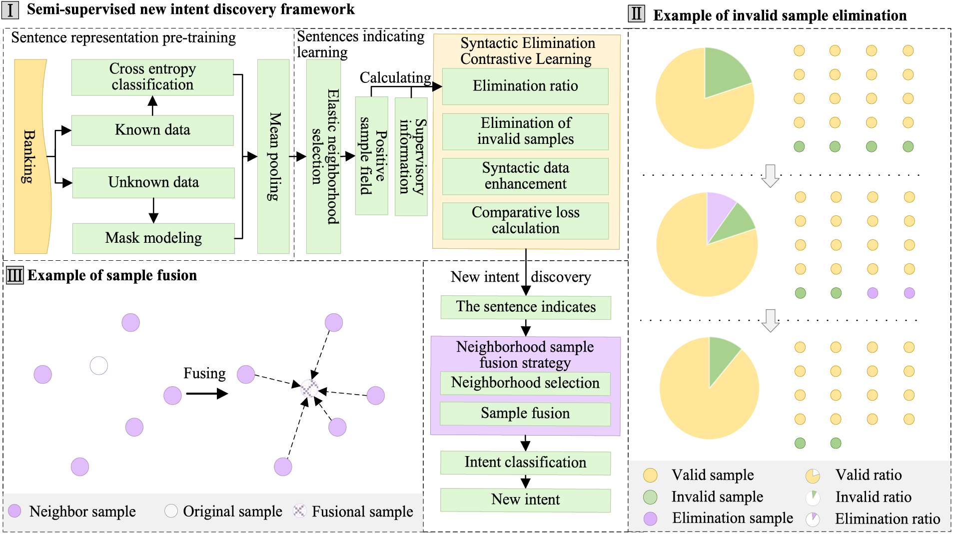
Figure 1: The SNID-ENSEF model framework

In Fig. 1, the framework is divided into three parts. The first part presents the Semi-supervised New Intent Discovery Framework, which includes sentence representation pre-training, sentence indicating learning, and new intent discovery. Sentence representation pre-training uses the Banking dataset, containing both labeled “known data” and unlabeled “unknown data.” For the known data, a cross-entropy classification task is performed, while for the unknown data, a mask prediction task is used. Both tasks are pre-trained jointly with outputs pooled from the pooling layer. Sentence indicating learning applies elastic neighborhood selection, where the neighborhood radius is determined by an elastic algorithm. The positive sample domain is refined by calculating an elimination ratio using supervised information to reduce ineffective samples. Data augmentation replaces verbs with semantically similar ones to enhance data diversity, followed by the computation of contrastive learning loss to complete the sentence representation training. For new intent discovery, the trained model generates sentence representations, which are processed through a nearest-neighbor fusion strategy. The nearest-neighbor domain size is selected, and samples are fused to obtain the final representation. Intent classification algorithms are then used to discover new intents and form new intent clusters. The second part illustrates the Example of Invalid Sample Elimination, showing the proportion of ineffective and effective samples in a pie chart, where two ineffective samples are eliminated from a total of 20, increasing the proportion of effective samples. The third part depicts the Example of Sample Fusion, where the Neighbor Sample represents the neighboring domain, the Original Sample is the pre-fusion sample, and the Fusional Sample is the resulting fused sample. A sample’s neighborhood is selected and fused using mean aggregation to improve the accuracy of the representation.

2.1 Sentence Representation Pre-Training

High-quality sentence representation is essential for accurate new intent discovery. Multi-task pre-training is conducted using the BERT model to adapt representations for this task, integrating masked language modeling and sentence classification. Through predicting missing words and classifying sentences, the model learns intent-aware representations, enhancing its ability to handle unseen topics and diverse intents. The core of masked language modeling is to mask certain words in a sentence and predict them based on the remaining context. This process enables the model to capture both the semantics of intent-related words and the overall sentence structure. An illustration of this task is shown in Fig. 2.

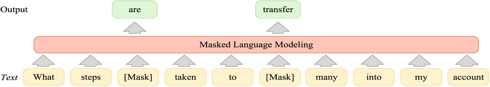
Figure 2: The illustration of the masked language modeling task

In Fig. 2, text denotes the text input to the model, the words in the sentence are masked partially using a random masking strategy, and the predicted words are output after model modeling. Predicting masked words in a sentence allows the model to understand the internal structure of the sentence and learn sentence information. The equation of loss is shown below:

(1)

where denotes the masked prediction probability distribution, denotes the predicted word, denotes the masked sentence, and is the number of masked words. The loss in masked tasks is reduced. The ability to predict masked words using sentence context is improved. Sentence dependencies are captured more effectively. The core idea is for the classification task to generate deep feature representations of the sentences. The corresponding sentence label is then calculated. Key features of the text are extracted during the classification process. Sentence comprehension is improved. The illustration of the classification task is shown in Fig. 3.

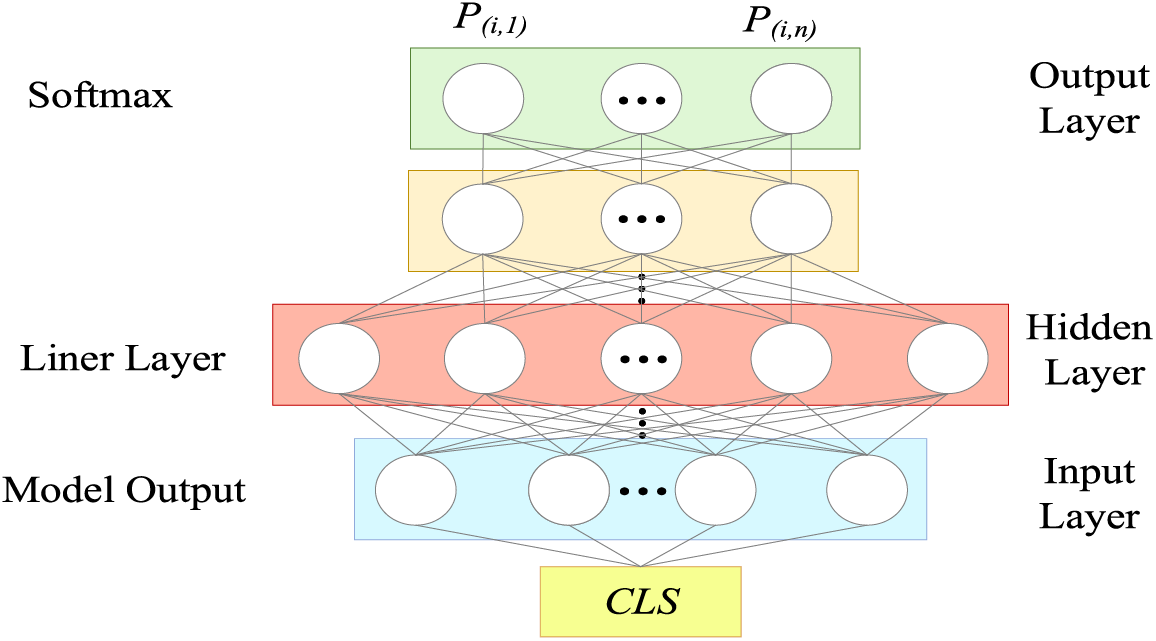
Figure 3: The illustration of classification task

In Fig. 3, CLS is the output of the model, Model Output is the model output layer, Liner Layer is the linear layer, and Softmax is the normalization layer. The CLS output from the model is fed into a linear layer. Several linear layers reduce the high-dimensional features to match the number of classes. A Softmax layer normalizes the probabilities to a range between 0 and 1. The classification probability is obtained. Combined with the class label, it is then processed through cross-entropy loss for calculation. The equation of cross-entropy classification loss is shown below:

(2)

where is the number of categorized samples, C is the number of categories, is a symbolic function (0 or 1), indicating that the true category of sample n is equal to c takes 1. Otherwise it takes 0, which is the predicted probability that sample n belongs to the category. The masked language modeling loss is added to the classification loss, resulting in the total multi-task pre-training loss . The equation of is shown below:

(3)

where denotes the loss of the masked language modeling task, and denotes the loss of the classification task. Joint training of the two tasks helps prevent the SNID-ENSEF model from overfitting on a single task or data type. A balanced optimization across different tasks results in effective initial sentence representations, providing a solid foundation for subsequent training. The final layer of the SNID-ENSEF model connects to a mean pooling layer, preserving overall semantic information. The representation vectors for each word are averaged, producing a sentence vector that captures the combined semantic information of the words in the sentence. The equation of the pooled representation is shown below:

(4)

where represents the number of word vectors, denotes the feature vector of a word, and indicates the position of the word vector. Mean pooling is applied to the word vectors by calculating the average representation of all words. The influence of random or irrelevant words is reduced on the overall representation. The overall representation improves stability and mitigates noise to some extent. The process facilitates subsequent training and the discovery of new intents.

Multi-task pre-training allows the SNID-ENSEF model to learn data features from different perspectives. The distinguishability of sentence representations is enhanced, and understanding of intent domain sentences is improved. The pooling layer outputs sentence representations, reducing the impact of noise and reinforcing stability.

2.2 Sentence Representation Learning

After multi-task pre-training, universal intent sentence representations are obtained, but they lack task-specific optimization for new intent discovery. To address this, a syntactic contrastive learning approach is proposed. First, syntactic elimination increases the proportion of valid samples in the positive sample domain by removing invalid ones, improving training efficiency. This is akin to clearing clutter, allowing the model to focus on relevant data. Second, syntactic data augmentation enriches sample diversity, introducing varied representations within the same category. Together, these strategies help the model more effectively locate useful samples and benefit from enhanced sample diversity, improving new intent discovery.

The selection method for positive samples is crucial in contrastive learning. A semi-supervised approach is used to maximize the number of positive samples for training. Supervised information is combined to flexibly adjust the neighborhood radius of positive samples and define the positive sample domain. The elastic neighborhood radius R is chosen to maximize the number of positive sample domains while minimizing the boundary of ineffective samples. The significance of finding the elastic neighborhood radius lies in identifying the optimal region around each sample to balance useful data with minimal irrelevant noise, ensuring more accurate intent classification. Within an appropriate elastic neighborhood radius, only the most relevant data surrounding each example is included. This process is akin to continuously zooming in or out until the optimal level of detail is achieved. The selection of the elastic neighborhood radius R is shown in Fig. 4.

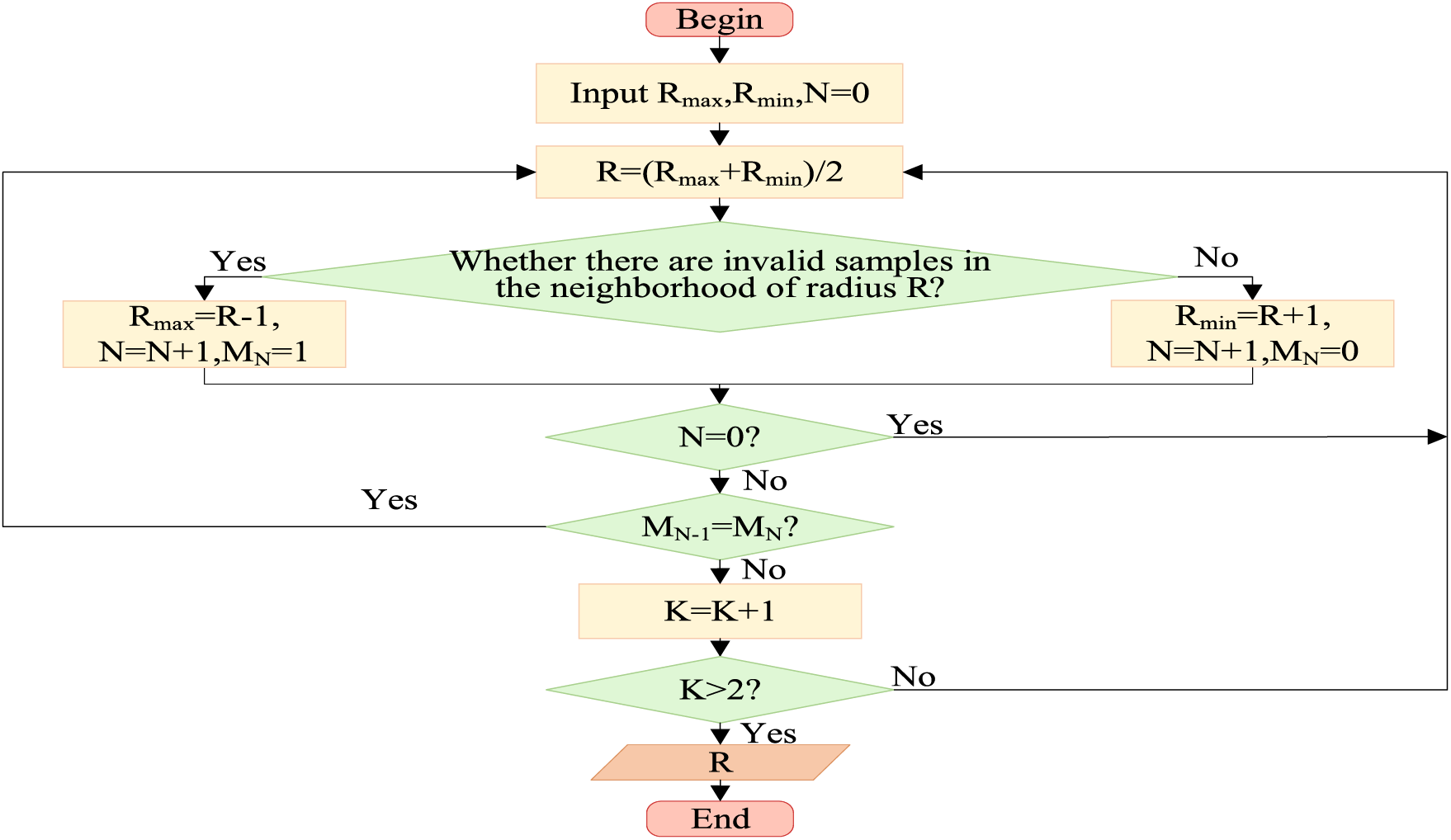
Figure 4: The selection of the elastic neighborhood radius R

In Fig. 4, R represents the elastic neighborhood radius, N denotes the number of iterations, and MN is a variable indicating whether invalid samples exist in the neighborhood during the N-th iteration. When M is 0, it means there are no invalid samples in the neighborhood, and when M is 1, it means there are invalid samples in the neighborhood. K represents the state change counter. When K is greater than 2, it indicates that the neighborhood radius has undergone a large-small-moderate or small-large-moderate state change, meaning R is the appropriate neighborhood radius. N is equal to 0 and used to check whether the loop has run at least once. During the first iteration of the loop, there is no historical state, so the comparison of states is skipped. The overall process begins by calculating the upper and lower bounds of the elastic neighborhood radius R as the initial input. A binary search method is used to find the appropriate neighborhood radius. If invalid samples are found within the radius R, the radius is reduced until no invalid samples are present. Then, R is increased until invalid samples are just present. If no invalid samples are found within the neighborhood of radius R, R is first increased until invalid samples are present, then decreased until no invalid samples are found. The illustration of the elastic neighborhood radius R is shown in Fig. 5.

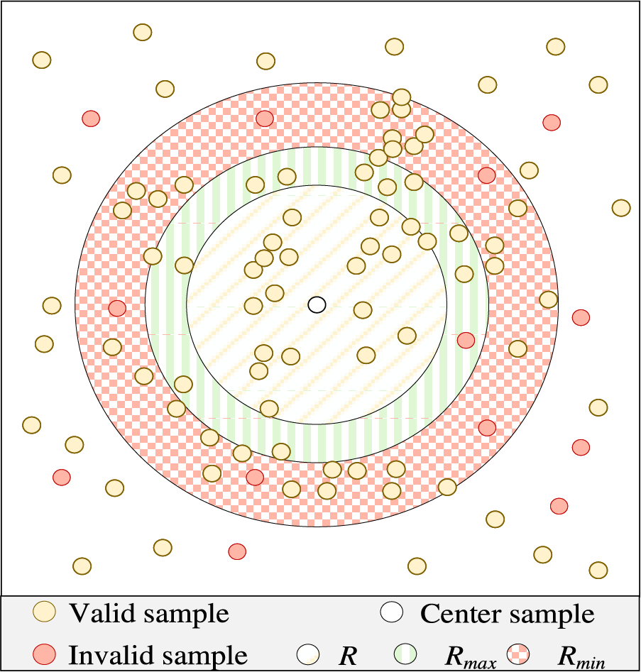
Figure 5: The illustration of the elastic neighborhood radius R

In Fig. 5, yellow samples represent valid samples, while green samples represent invalid samples. The orange cross-circles indicate that the radius is too large, causing too many invalid samples in the neighborhood. The yellow dashed circles represent a slightly smaller neighborhood radius, which cannot include as many valid samples as possible. The green circles represent the appropriate neighborhood radius. If the judgment condition is K < 1, the green circle cannot be obtained, and the search will always fall into ranges that are either too large or too small. Therefore, the judgment condition is set to , allowing for an adjustment after the radius becomes too large or too small.

Due to the presence of ineffective samples in the positive sample domain and a more significant number of unknown ineffective samples, supervised information is used to calculate the number of ineffective samples in the selection strategy and to remove the ineffective samples from the supervised portion. The number of ineffective samples is then used to estimate the ineffective sample ratio in the positive sample domain and to calculate the reduction sample rate. It ensures that after the elimination of positive samples, the overall ineffective sample ratio increases, improving the training effectiveness of syntactic contrastive learning. Before the elimination of ineffective samples, the equation of the sample efficiency under the initial elastic neighborhood radius R is shown below:

(5)

where represents the total number of samples, and denotes the estimated number of ineffective samples. The process of eliminating ineffective samples can be understood as extracting L samples from samples. After extracting L samples, the proportion of effective samples in the total can fall into three scenarios. Remaining unchanged, decreasing, or increasing. When L samples are extracted, and Q effective samples are present, the efficiency remains unchanged. The equation for calculating Q is shown below:

(6)

where represents the total number of samples, denotes the estimated number of ineffective samples, indicates the efficiency of the elastic neighborhood samples, and L signifies the number of samples to be eliminated. When L samples are extracted, and the number of effective samples is greater than Q, the efficiency after extraction is less than that before extraction. The equation for calculating the probability is shown below:

(7)

where represents the probability of having e-positive samples in the eliminated samples, and the summation indicates the cumulative probability. When the number of extracted effective samples is less than Q, the efficiency after extraction is lower than that before extraction. The equation for calculating the probability is shown below:

(8)

where represents the probability of extracting e-positive samples, and the summation indicates the cumulative probability. After calculating the probabilities, L is taken when the probability exceeds 50%. The negative impact of ineffective samples on training effectiveness far exceeds the benefits of a low proportion of additional effective samples. Therefore, when the extraction probability exceeds 50%, the overall training performance of the model is improved. The equation for calculating the reduction rate is shown below:

(9)

where L represents the number of eliminated samples, and denotes the total number of samples. The equation for calculating the positive sample domain is shown below:

(10)

where represents the original positive sample domain, and denotes the reduction rate. It indicates that the positive sample domain is eliminated with a probability of . After obtaining a suitable positive sample domain, data augmentation is applied to the positive samples using a combination of syntactic data enhancement and random token replacement. Data augmentation increases the diversity of the training data, enhancing the model’s ability to recognize sentences. The positive sample data augmentation is shown in Fig. 6.

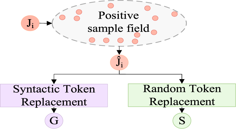
Figure 6: The positive sample data augmentation

In Fig. 6, represents the i training sample, denotes the positive sample uniformly selected from positive sample domain, G indicates the sample after syntactic data augmentation, and S represents the sample after random token replacement. The specific operation of syntactic data augmentation involves two steps. The first step considers syntactic factors in selecting verbs as replacement words, and the second step involves choosing synonyms for substitution. Using the sentence “What steps are taken to transfer many into my account” as an example, it demonstrates how syntactic augmentation selects and replaces syntactic tokens. An example of syntactic replacement is shown in Fig. 7.

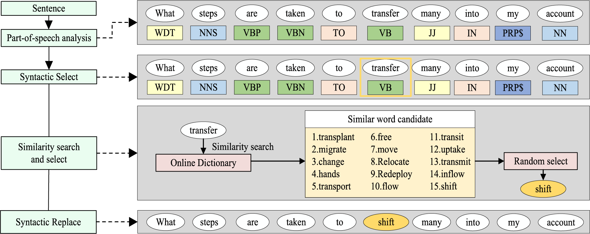
Figure 7: The illustration of syntactic replacement

In Fig. 7, the original sentence is analyzed using Stanza CoreNLP [33] for part-of-speech tagging, obtaining the part-of-speech for each word in the sentence, such as ‘VB’ for verbs and ‘NN’ for nouns. ’Syntactic Select’ refers to the process of selecting the word with the part-of-speech tag ‘VB’ (the word ‘transfer’). “Similarity search and select” refers to searching for the list of candidate words with the highest semantic similarity to the selected word. Using an open-source online dictionary [34], a semantic similarity search is performed for the word ‘transfer,’ identifying the 15 most semantically similar words as candidates for replacement. One word is randomly selected from this list to replace the word in the VB position. This results in the syntactically augmented sentence. The illustration of random token replacement is shown in Fig. 8.

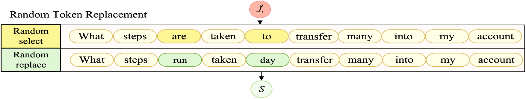
Figure 8: The illustration of random token replacement

In Fig. 8, ‘Random select’ refers to the random selection of positions for replacement words, while ‘Random replace’ indicates the process of completing data augmentation using randomly selected words for substitution. By applying both syntactic enhancement and random replacement strategies to the sentences, positive samples for data augmentation are obtained. Subsequently, syntactic elimination contrastive learning is used to train the model. The equation of syntactic elimination contrastive learning loss is shown below:

(11)

where represents the number of samples, denotes the sample index, is the sentence embedding of the -th sample, is the index of the negative sample for , S is the sentence embedding of sample after random replacement, G is the sentence embedding of sample after syntactic data augmentation, and is the -th embedding of the negative pair after augmentation. is the temperature parameter, and is the similarity function on the normalized feature vectors.

The model optimizes syntactic elimination contrastive learning to cluster sentences with the same intent, reducing representation differences and achieving a more compact distribution in vector space. Conversely, it maximizes differences between representations of different intents, creating a more dispersed distribution. This adjustment of sentence representations establishes a solid foundation for new intent discovery.

2.3 New Intent Discovery

In new intent discovery, the distance between samples of the same intent is key to accurate intent identification. Large intra-class distances can separate similar intent samples, while small inter-class distances may cause misclassification. To address this, a neighborhood sample fusion strategy replaces sample vectors with the mean of their neighborhood vectors, reducing noise and outliers. This results in more compact representations, decreasing intra-class distance while increasing inter-class distance, thereby improving intent recognition accuracy. This enhances the accuracy of new intent discovery. The illustration of the neighborhood sample fusion strategy is shown in Fig. 9.

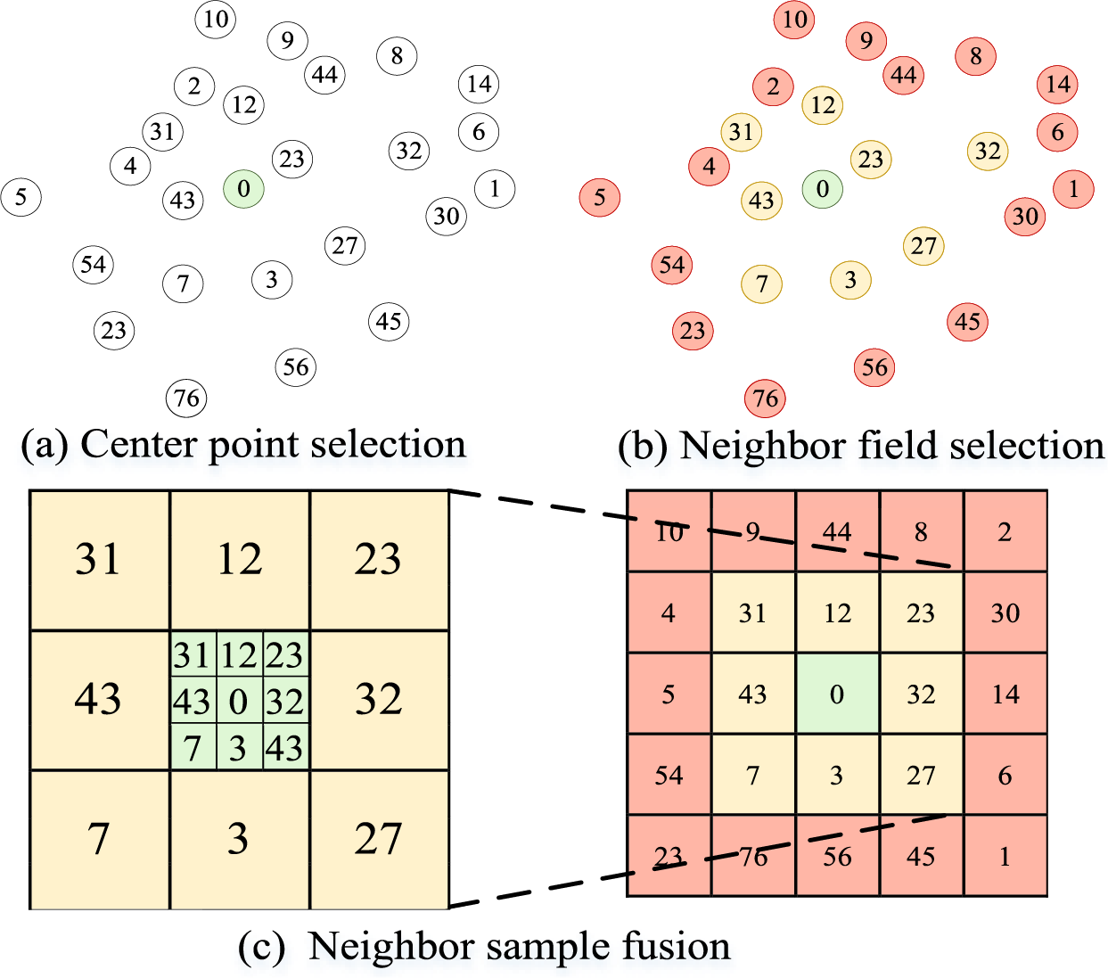
Figure 9: The illustration of the neighborhood sample fusion strategy

In Fig. 9, the numbers represent sample indices. In Fig. 9a, the samples to be tested are selected as the central samples. The neighborhood sample fusion strategy is applied to the green sample with index 0, selecting the k nearest-neighbors of the 0-th sample vector. In Fig. 9b, the size of the sample neighborhood is determined based on the elastic neighborhood selection strategy. The yellow samples are the neighbors of the green sample at index 0, while the pink samples represent other samples surrounding the green sample. In Fig. 9c, the 0-th sample is replaced with the mean of its neighbor samples. The equation of the mean of the sample vectors is shown below:

(12)

where represents the number of nearest-neighbor samples, is the index of the nearest-neighbor sample, and denotes the vector of the -th neighbor sample. The neighborhood sample fusion strategy in creating cohesive clusters is based on the idea of similarity and adjacency, which is akin to placing similar items closer together. This reduces disorder and improves the accuracy of intent detection. The neighborhood can be compared to the classification areas in a library, where books on similar topics are placed in the same area, making it easier to find books on related subjects quickly. This helps the model recognize new intents more efficiently. As a result, the determination of sample similarity becomes more reliable, effectively lowering the difficulty of new intent discovery and aiding in the more accurate identification and definition of new intent categories. After determining the number of new intents, a similarity measurement method is employed to classify the intent sentence vectors into new intent categories. An initial label selection algorithm is then used to choose intent sentences as pseudo-labels for these new intent classes [32]. The remaining sentences are categorized into their respective new intent classes using similarity measures. The equation of the new intent class is shown below:

(13)

where denotes the ordinal number of the smallest value in the range in which the function is taken. calculate the spatial distance between the vectors. denotes the vector of unclassified intent sentences. denotes the vector of intent sentences for the -th pseudo-label.

The SNID-ENSEF model achieves the ability to represent intent sentences through multi-task pre-training and fine-tuning with contrastive learning, resulting in a uniform distribution of intent sentences within the vector space. New intent classes are obtained using a similarity classification method.

3  Experimental Results and Analysis

3.1 Experimental Environment and Datasets

Model development and experiments are conducted on a cloud server, with an Nvidia GeForce RTX 3090 GPU utilized for training the BERT model. The Adam optimizer is utilized, and experiments are conducted with the Python programming language and the PyTorch framework. The versions are used Python 3.8.18, PyTorch 1.12.0, and CUDA 11.3. The experimental hyperparameter settings are as follows. The learning rate (Lr) is set to 1e-5, the batch size (Bs) is set to 128, the number of training epochs (Ep) is set to 50, and the elimination rate (p) is set to 0.05. The SNID-ENSEF model is tested on three publicly available intent datasets. Banking77 is a dataset of banking dialogues containing 77 intents derived from conversations in the banking context. StackOverflow is a large-scale dataset collected from an online Q & A platform. Clinc150 encompasses a wide range of user intents and scenarios, not limited to specific domains [32].

3.2 Evaluation Indicators

To evaluate the performance of the models Adjusted Rand Coefficient (ARI), Accuracy (ACC), and Normalized Mutual Information (NMI) are used to evaluate the performance of the SNID-ENSEF model as well as to compare the models [35]. Adjusted Rand coefficients are used to measure the degree of similarity between the categorization results and the real situation. Accuracy is used to measure the proportion of accurate categorization. Normalized mutual information measures the consistency between the categorization results and the real labels. The three evaluation indicators are distributed in [0, 1], with larger values representing more accurate categorization results.

3.3 Attention Headcount Analysis

In syntactic elimination contrastive learning, the magnitude of the elimination rate significantly impacts the effectiveness of training samples. To verify the rationale behind the chosen elimination rate, the effects of different elimination rates on the SNID-ENSEF model are examined. Five elimination rates ranging from 0.01 to 0.05 are selected around the optimal elimination rate, with the evaluation metrics displayed for the Stackoverflow dataset. The illustration of elimination rate variation is shown in Fig. 10.

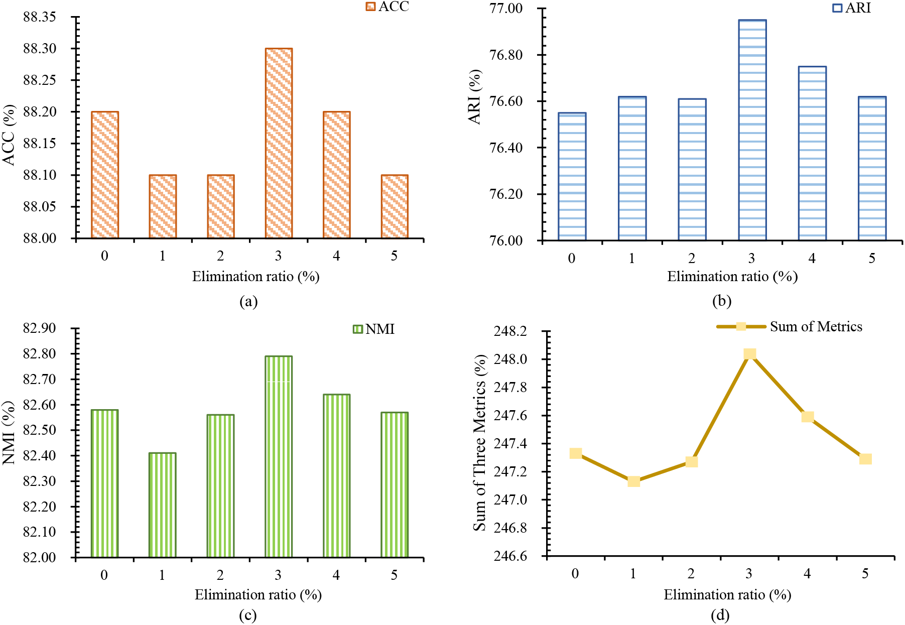
Figure 10: The illustration of elimination rate variation

In Fig. 10, the model performs best at an elimination rate of 0.03. Fig. 10a shows the change in the ACC index with the elimination rate. Fig. 10b shows the change in the ARI index with the elimination rate. Fig. 10c shows the change in the NMI index with the elimination rate. Fig. 10d shows the change of the sum of the three indicators with the elimination rate. The choice of elimination rate significantly impacts the effectiveness of the model’s training samples. When the elimination rate is too low, the effectiveness of the training samples may decrease or remain unchanged, failing to eliminate the training interference from invalid samples. Conversely, if the elimination rate is too high, the model may incorrectly remove valid samples, leading to a reduction in effective training data and overall poorer model performance. Therefore, selecting an elimination rate of 0.03 strikes a balance between removing invalid samples and retaining valid ones, providing the model with an adequate training dataset, which helps enhance its performance and generalization ability.

3.4 Learning Rate Analysis

To select an appropriate parameter k for the neighborhood sample fusion strategy, the effects of different k values on the SNID-ENSEF model are examined. Values near the ten best k values are used. The variations in SNID-ENSEF model metrics under different parameters of the neighborhood sample fusion strategy are shown in Fig. 11.

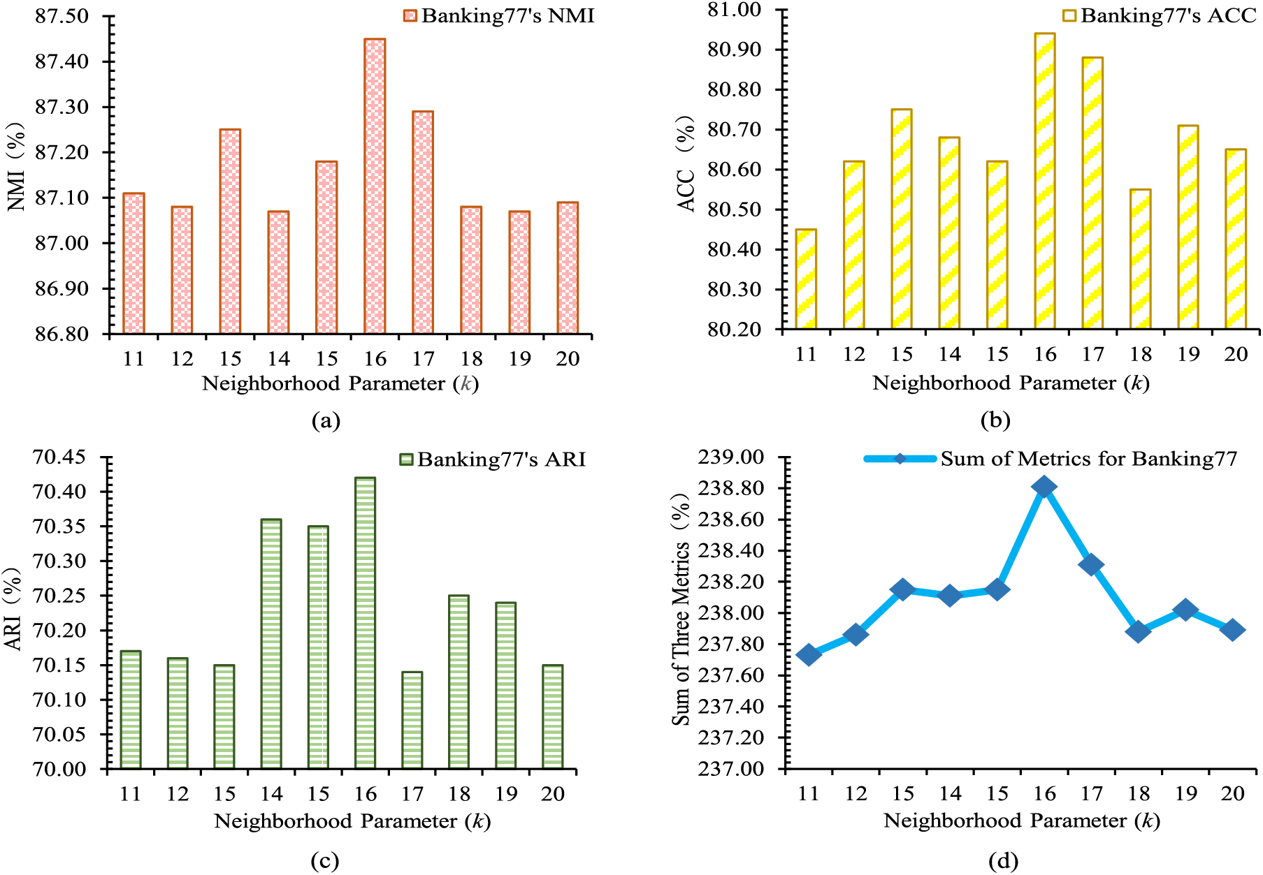
Figure 11: Variation of metrics with different neighbors k in Banking77

In Fig. 11, differences in model performance are observed under various settings of k. Fig. 11a shows the change in the NMI index with k. Fig. 11b shows the change of ACC index with k. Fig. 11c shows the change in the ARI index with k. Fig. 11d shows the change in the sum of the three indicators with k. When k is too small, the neighborhood sample fusion strategy fails to filter out noise. Conversely, if k is too large, new noise may be introduced, which prevents the stabilization of new intents toward their respective classes, ultimately hindering the achievement of optimal results. Based on the experimental results, an appropriate k value is chosen to achieve effective outcomes.

3.5 Ablation Experiments

The SNID-ENSEF model is primarily divided into the syntactic elimination contrastive learning module (SECL) and the neighborhood sample fusion strategy module (NSFS).SECL contains Syntactic augmentation (SA) and Elastic neighborhood elimination (ENE). Different stage combinations are used in the StackOverflow dataset. An ablation study is conducted to analyze the SNID-ENSEF model. The ablation experiments validate the effectiveness of the syntactic elimination contrastive learning module and the neighborhood sample fusion strategy module. The selection of modules for SNID-ENSEF ablation experiments is shown in Table 1.

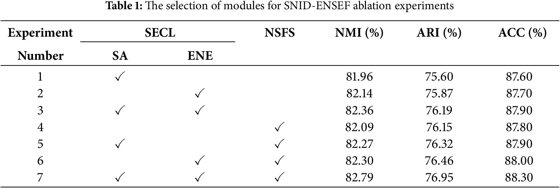
In Table 1, Experiment 1 involves only using syntactic enhancement. Experiment 2 focuses solely on elastic neighborhood ablation. Experiment 3 combines both syntactic enhancement and elastic neighborhood ablation. Experiment 4 utilizes only the neighborhood sample fusion strategy. Experiment 5 implements a combination of syntactic enhancement and neighborhood sample fusion. Experiment 6 pairs elastic neighborhood ablation with neighborhood sample fusion. Finally, Experiment 7 represents the full SNID-ENSEF model, which employs both syntactic ablation contrastive learning and neighborhood sample fusion strategies.

Experiments 1–3 show that elastic neighborhood elimination outperforms syntactic enhancement in syntactic elimination contrastive learning. While data augmentation enriches sample diversity, elastic neighborhood elimination fundamentally increases the proportion of effective samples, improving data efficiency. Thus, it provides more valid training data. Both methods contribute to expanding training data, and their combination enhances sentence understanding and new intent recognition accuracy. Experiment 4 demonstrates that neighborhood sample fusion significantly aids in recognizing new intents. Experiments 5–6 confirm that combining syntactic elimination contrastive learning with neighborhood sample fusion achieves a more uniform distribution and that elastic neighborhood elimination is more effective than syntactic enhancement. The ARI, ACC, and NMI of syntactic elimination comparative learning are higher than those of the neighborhood sample fusion strategy module. In the absence of syntactic elimination comparative learning, the ACC value decreased by 0.41% compared to the results with both modules. When the density distribution-aware comparative learning module is missing, the ACC value drops by 1.68%. In conclusion, the two modules introduced in the study significantly contribute to the accuracy of new intent discovery. The ablation experiments of random token replacement (RTR) and syntactic token replacement (STR) are shown in Table 2.

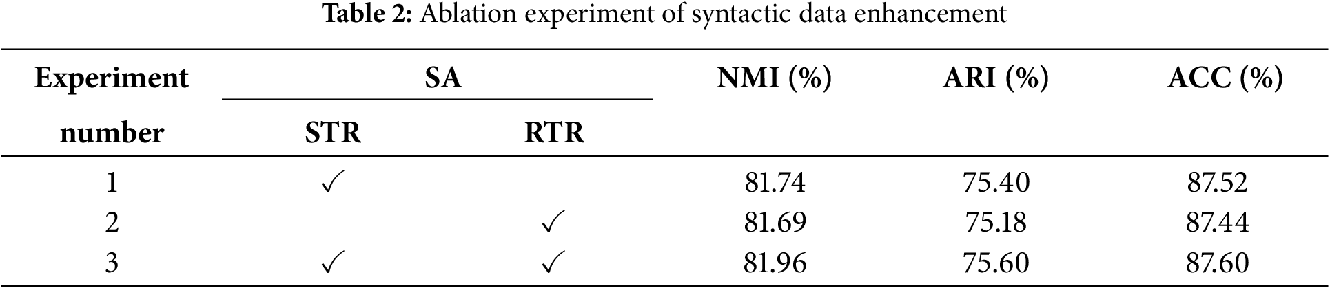
In Table 2, the experimental results show that SRT significantly outperforms RRT, while RRT shows a relatively smaller improvement. However, when combined, SRT enhances sentence diversity, while RRT introduces some appropriate noise, improving the model’s robustness and leading to better performance.

3.6 Comparison Experiments

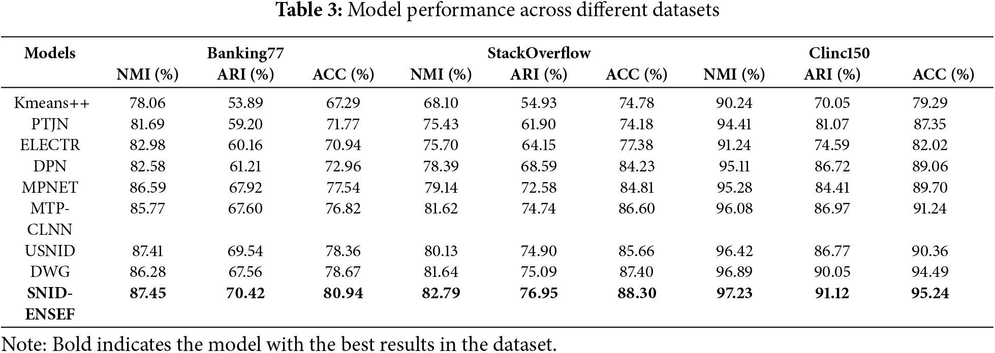
To evaluate the performance of the proposed SNID-ENSEF model, comparative experiments are conducted on the Banking77, Stackoverflow, and Clinc150 datasets. The benchmark models for comparison include: Kmeans++ [36]: A traditional clustering algorithm that improves the initialization of cluster centroids. PTJN [37]: A robust pseudo-label training and source domain joint training network. Noisy pseudo-labels are refined using prior knowledge, and a new extractor-generator-corrector architecture is introduced. ELECTR [38]: A Transformer-based language representation pre-training model that draws on the ideas of GANs. It trains the model by distinguishing between real words and “fake” words generated by a small generator model. DPN [39]: An end-to-end deep contrastive clustering algorithm. The algorithm jointly updates model parameters and clustering centers through supervised and self-supervised learning, optimizing the use of labeled and unlabeled data. MPNET [40]: A new pre-training model that improves traditional pre-training methods through a “Masked and Permuted Pre-training” strategy. MTP-CLNN [35]: A multi-task pre-training model for new intent discovery has been proposed. Utilizing self-supervised signals in the representation space to improve the accuracy of new intent discovery. USNID [41]: A new intent discovery model that introduces a centroid-guided clustering mechanism. DWG [32]: A new intent discovery model that employs a novel diffusion-weighted graph framework. This framework uses a weighted method based on semantic similarity and local structure for contrastive learning.

As shown in Table 3, the SNID-ENSEF model exhibits strong performance in terms of NMI, ARI, and ACC across the Banking77, StackOverflow, and Clinc150 datasets. Compared to the highest-performing models (DWG) in terms of NMI, ARI, and ACC from Kmeans++, PTJN, ELECTR, DPN, MPNET, MTP-CLNN, USNID, and DWG, the SNID-ENSEF model shows improvements of 1.17%, 1.15%, and 0.34% in NMI, 0.88%, 1.86%, and 1.07% in ARI, 2.27%, 0.9%, and 0.75% in ACC, respectively. The training of the SNID-ENSEF model utilizes elastic neighborhood boundaries to select positive sample domains, ensuring a high quantity of training data while eliminating ineffective samples to enhance sample efficiency. Additionally, by referencing syntactic information and substituting meaningful words in sentences, the model increases the diversity of training samples, thereby improving training effectiveness. The use of the neighborhood sample fusion strategy reduces noise and decreases the difficulty of the new intent discovery task. By combining these approaches, the SNID-ENSEF model learns high-quality intent sentence representations from limited training samples, enhancing the accuracy of the new intent discovery task.

4  Discussion

4.1 Generalized Performance Test

To validate the generalization ability of the model, two additional datasets were introduced to evaluate its performance across different domains. MCID [42]: An open-source intent detection dataset for COVID-19 chatbots focusing on the healthcare domain. It contains sixteen intents and is used to test the applicability of the model in the medical field. HWU64 [43]: A dataset consisting of 25716 utterances across 21 domains and 64 intents. Compared to Clinc, which has fewer domains, HWU64 enables the testing of the performance of the model across a broader range of domains. The results are presented in Table 4.

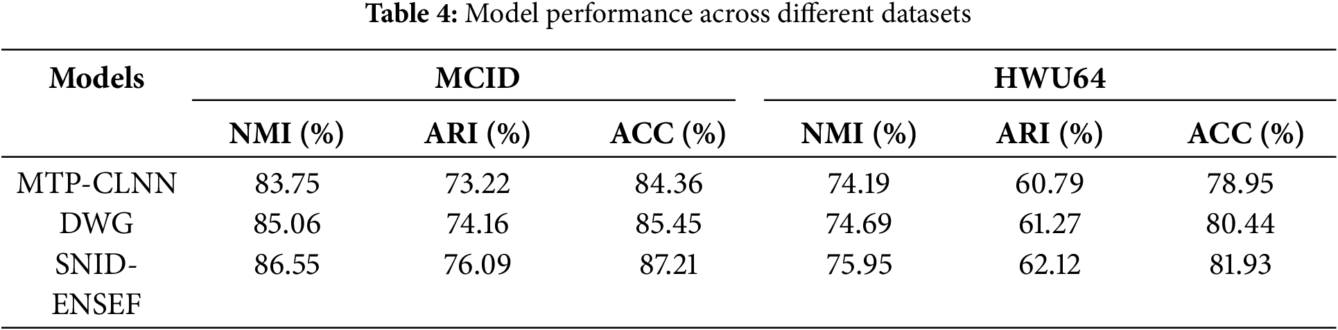
As shown in Table 4, the ESEF-SNID model demonstrates an improvement over models such as DWG and MTP-CLNN, exhibiting stable performance across different datasets. This stability to some extent validates the generalization capability of the ESEF-SNID model.

4.2 Expectations and Future Prospects

With the rapid development of large language models, an increasing number of task-specific models are being enhanced by these large models. Integrating large language models will further improve the performance of models on specific tasks. For the ESEF-SNID model, leveraging large language models can refine the distinction of previously unknown intents, allowing for a more detailed differentiation of broadly separated intents, thereby increasing the accuracy of intent discovery. Another future direction involves converting newly discovered intents into defined intents. However, this process requires significant human effort and computational resources. Therefore, integrating large language models to assist in defining discovered intents is a crucial area that needs to be addressed in future work.

4.3 Practical Application

Virtual assistants are able to respond to users’ questions. The application of new intent discovery in virtual assistants enables them to provide appropriate replies to various user inquiries, allowing them to more intelligently address a wide range of user needs without being limited by predefined tasks. This increase in flexibility has a profound impact on user satisfaction and interaction experience, making conversations more engaging and open-ended. For example, when a home voice assistant encounters a newly introduced term for the first time, it may not provide an effective response because it cannot recognize the meaning of the new term. However, through the discovery of new intent, the assistant can capture this intent, allowing it to provide appropriate replies in the future when the term or its associated intent is mentioned again.

4.4 Discussion of Marginal Cases

To discuss the ability of the SNID-ENSEF Model to recognize intent meaning overlap and intent sentence similarity, two major overlapping intent categories in the Banking dataset Card and Transaction intents-were extracted into four sub-overlapping intents, resulting in a total of twenty-nine categories. The performance of DWG and SNID-ENSEF was then tested in extreme cases. The dataset labels and intent distribution are shown in Table 5. The model performance is shown in Table 6.

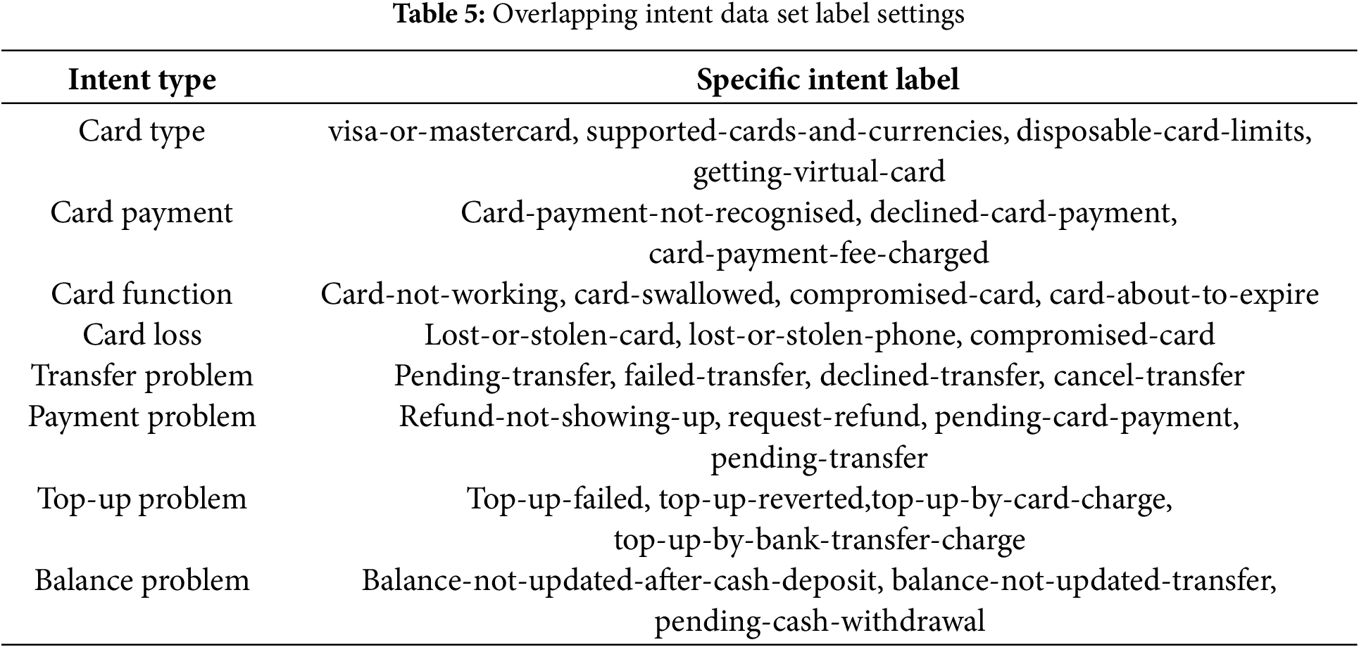
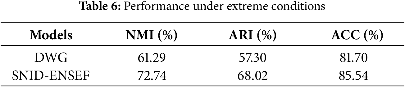
As shown in Table 6, in extreme cases, SNID-ENSEF outperforms the strongest competing model, DWG, in the NMI, ARI, and ACC metrics. This indicates that SNID-ENSEF still retains a certain ability to recognize intents even under extreme conditions.

4.5 Real-Time Performance Index

To test the model’s actual performance, SNID-ENSEF and the DWG model were tested on the BANKING dataset, and real-time performance metrics were recorded for comparison. The experimental results are shown in Table 7.

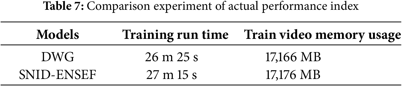
As shown in Table 7, compared to the DWG model, the SNID-ENSEF model is 50 s slower. However, thanks to the matrix operations used in the proposed method, this time difference is within an acceptable range. The memory usage increased by 10 MB without any trade-off between space and performance. Overall, the SNID-ENSEF model does not have significant disadvantages in terms of time and memory usage compared to the strongest competing model while showing an improvement in performance.

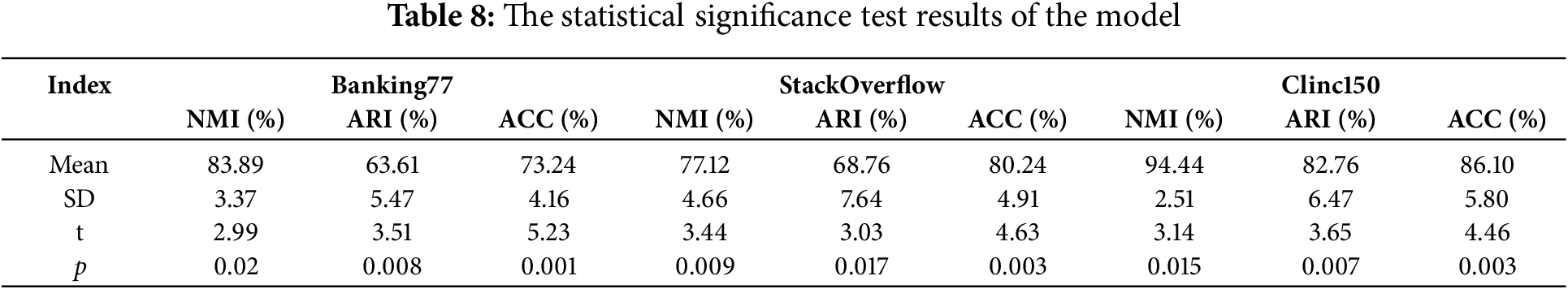
4.6 Statistical Significance Test

Perform significance testing on the model’s various metrics to verify the performance improvement of the SNID-ENSEF model compared to other competing models. The formula for the -test is as follows:

(14)

where X represents the data point to be tested, represents the mean of the other data, SD represents the standard deviation, and represents the number of data points. Calculate the mean and standard deviation of the metrics listed in Table 3 to compute the t-value. Then, obtain the -value from the corresponding t-distribution. Set the null hypothesis: There is no significant difference between the SNID-ENSEF model and the competing models. Set the alternative hypothesis: there is a significant difference between the metrics of the SNID-ENSEF model and the other competing models. Reject the null hypothesis if the p-value is less than 0.05. The specific calculations are as follows.

As shown in Table 8, the -values for all metrics of the SNID-ENSEF model are less than 0.05 compared to the competing models, allowing us to reject the null hypothesis. Additionally, the silhouette scores for the strongest competing model, DWG, and the SNID-ENSEF model are calculated. The silhouette score of the DWG model is 0.6811, while the silhouette score of the SNID-ENSEF model is 0.8755, further validating the performance improvement of the SNID-ENSEF model.

4.7 Select Radius Adjustment Thresholds and Parameters

In order to fully demonstrate the initial value selection and parameters of the elastic neighborhood strategy, a set of 669 samples is taken, and the Euclidean distance from the first sample to all other samples is calculated. For the sake of convenience, the Euclidean distances in this paper are scaled by a factor of 1000. The relationship between the samples and their distances is shown in Fig. 12.

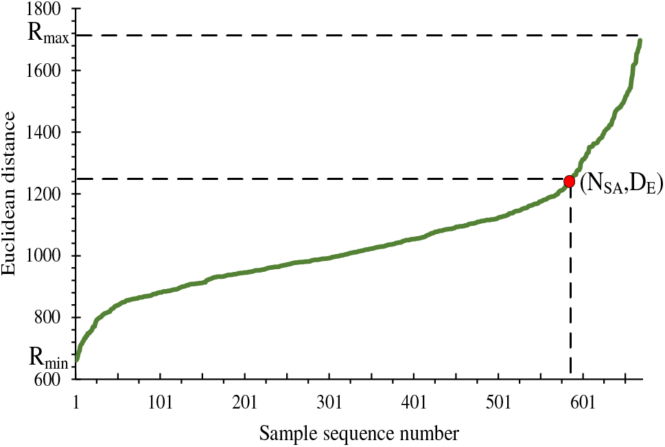
Figure 12: The relationship between sample and distance

In Fig. 12, the distances between the first sample and all other samples are plotted, where the minimum distance is denoted as . At this point, the neighborhood of the sample contains only one sample, and there are no invalid samples. The maximum distance is denoted as , at which point the neighborhood contains all samples, and there are certainly invalid samples. This choice of values ensures that the elastic neighborhood strategy will have a solution. The change in the value of R after the judgment process is determined by the following formula:

(15)

In the distance range close to 600, where 600 samples are distributed, is approximately 1. Therefore, the value of R is adjusted as R+1 or R−1.

5  Conclusion

In dialogue generation, discovering new intents from unknown ones can enhance the ability to recognize unknown intents and advance the development of dialogue generation. A Semi-supervised New Intent Discovery for Elastic Neighborhood Syntactic Elimination and Fusion model (SNID-ENSEF) is proposed in this paper. By employing syntactic elimination comparative learning and syntactic data augmentation to introduce true synonyms, the richness of training samples is enhanced, allowing the model to learn intent sentence features. Ineffective samples are eliminated through the elastic selection of positive sample domains. It significantly increases the quantity and effectiveness of training samples. As a result, the capabilities of sentence representation are improved. Additionally, sample noise is filtered out by the neighborhood sample fusion strategy. The transformation addresses the new intent classification problem. The difficulty of discovering new intents is reduced, which enhances the accuracy of new intent discovery. The experimental results indicate that the SNID-ENSEF model achieves average improvements of 0.88%, 1.27%, and 1.30% in the NMI, ACC, and ARI, respectively, compared to baseline models PTJN, DPN, MTP-CLNN, and DWG, demonstrating the superior intent discovery capabilities of the SNID-ENSEF model. In summary, researching semi-supervised intent discovery is essential. In daily life, SNID-ENSEF can make voice assistants more intelligent by remembering new things you mention and recognizing them, allowing for smoother responses in future conversations. In future work, integrating large language models to enhance the performance of SNID-ENSEF or using large models to define unknown intents recognized by the SNID-ENSEF model will be key areas we focus on.

Acknowledgement: The authors look forward to the insightful comments and suggestions of the anonymous reviewers and editors, which will go a long way towards improving the quality of this paper.

Funding Statement: This work is supported by Research Projects of the Nature Science Foundation of Hebei Province (F2021402005).

Author Contributions: The authors confirm contribution to the paper as follows: study conception and design: Di Wu, Liming Feng; data collection: Xiaoyu Wang; analysis and interpretation of results: Di Wu, Liming Feng, Xiaoyu Wang; draft manuscript preparation: Di Wu, Liming Feng. All authors reviewed the results and approved the final version of the manuscript.

Availability of Data and Materials: The datasets used or analyzed during the current study are available from the corresponding author, Di Wu, on reasonable request.

Ethics Approval: Not applicable.

Conflicts of Interest: The authors declare no conflicts of interest to report regarding the present study.

References

1. Singh GV, Firdaus M, Chauhan DS, Ekbal A, Bhattacharyya P. Zero-shot multitask intent and emotion prediction from multimodal data: a benchmark study. Neurocomputing. 2024;569(3):127128. doi:10.1016/j.neucom.2023.127128. [Google Scholar] [CrossRef]

2. Musto C, Martina AFM, Iovine A, Narducci F, de Gemmis M, Semeraro G. Tell me what you Like: introducing natural language preference elicitation strategies in a virtual assistant for the movie domain. J Intell Inform Syst. 2024;62(2):575–99. doi:10.1007/s10844-023-00835-8. [Google Scholar] [CrossRef]

3. Al-Besher A, Kumar K, Sangeetha M, Butsa T. BERT for conversational question answering systems using semantic similarity estimation. Comput Mater Contin. 2022;70(3):4763–80. doi:10.32604/cmc.2022.021033. [Google Scholar] [CrossRef]

4. Chandrakala C, Bhardwaj R, Pujari C. An intent recognition pipeline for conversational AI. Int J Inform Technol. 2024;16(2):731–43. doi:10.1007/s41870-023-01642-8. [Google Scholar] [CrossRef]

5. Devlin J, Chang MW, Lee K, Toutanova K. BERT: Pre-training of deep bidirectional transformers for language understanding, In: Proceedings of the 2019 Conference of the North American Chapter of the Association for Computational Linguistics: Human Language Technologies, Volume 1 (Long and Short Papers); 2019. p. 4171–4186. [Google Scholar]

6. Liu Y. RoBERTa: a robustly optimized bert pretraining approach. arXiv:1907.11692. 2019. [Google Scholar]

7. Sanh V. DistilBERT, a distilled version of BERT: smaller, faster, cheaper and lighter. arXiv:1910.01108. 2019. [Google Scholar]

8. Lan Z, Chen M, Goodman S, Gimpel K, Sharma P, Soricut R. ALBERT: a Lite BERT for self-supervised learning of language representations. arXiv:1909.11942. 2019. [Google Scholar]

9. Clark K, Luong MT, Le QV, Manning CD. ELECTRA: pre-training text encoders as discriminators rather than generators. arXiv:2003.10555. 2020. [Google Scholar]

10. Çelik A, Küçükmanisa A, Urhan O. Feature distillation from vision-language model for semisupervised action classification. Turkish J Electr Eng Comput Sci. 2023;31(6):1129–45. doi:10.55730/1300-0632.4038. [Google Scholar] [CrossRef]

11. Jin W, Zhao B, Zhang L, Liu C, Yu H. Back to common sense: oxford dictionary descriptive knowledge augmentation for aspect-based sentiment analysis. Inform Process Manag. 2023;60(3):103260. doi:10.1016/j.ipm.2022.103260. [Google Scholar] [CrossRef]

12. Yang R, Dai W, Li C, Zou J, Xiong H. NCGNN: node-level capsule graph neural network for semisupervised classification. IEEE Trans Neural Netw Learn Syst. 2022;35(1):1025–39. doi:10.1109/TNNLS.2022.3179306. [Google Scholar] [PubMed] [CrossRef]

13. Xiu Y, Ye F, Chen Z, Liu Y. Hybrid tensor networks for fully supervised and semi-supervised hyperspectral image classification. IEEE J Sel Top Appl Earth Obs Remote Sens. 2023;16:7882–95. [Google Scholar]

14. Yang M, Yang B, Liao M, Zhu Y, Bai X. Sequential visual and semantic consistency for semi-supervised text recognition. Pattern Recognit Lett. 2024;178(1):174–80. doi:10.1016/j.patrec.2024.01.008. [Google Scholar] [CrossRef]

15. Wang H, Qiu X, Tan X. Multivariate graph neural networks on enhancing syntactic and semantic for aspect-based sentiment analysis. Appl Intell. 2024;54(22):11672–89. doi:10.1007/s10489-024-05802-6. [Google Scholar] [CrossRef]

16. Zhao B, Jin W, Zhang Y, Huang S, Yang G. Prompt learning for metonymy resolution: enhancing performance with internal prior knowledge of pre-trained language models. Knowl Based Syst. 2023;279(3):110928. doi:10.1016/j.knosys.2023.110928. [Google Scholar] [CrossRef]

17. Wei J, Zou K. EDA: easy data augmentation techniques for boosting performance on text classification tasks. In: Proceedings of the 2019 Conference on Empirical Methods in Natural Language Processing and the 9th International Joint Conference on Natural Language Processing (EMNLP-IJCNLP); 2019; Hong Kong, China. p. 6382–8. [Google Scholar]

18. Zhao T, Liu Y, Neves L, Woodford O, Jiang M, Shah N. Data augmentation for graph neural networks. Proc AAAI Conf Artif Intell. 2021;35(12):11015–23. doi:10.1609/aaai.v35i12.17315. [Google Scholar] [CrossRef]

19. Whitehouse C, Choudhury M, Aji A. LLM-powered data augmentation for enhanced cross-lingual performance. In: Proceedings of the 2023 Conference on Empirical Methods in Natural Language Processing; 2023; Singapore. p. 671–86. [Google Scholar]

20. Thakur N, Reimers N, Daxenberger J, Gurevych I. Augmented SBERT: data augmentation method for improving Bi-encoders for pairwise sentence scoring tasks. In: Proceedings of the 2021 Conference of the North American Chapter of the Association for Computational Linguistics: Human Language Technologies; 2021. p. 296–310. [Google Scholar]

21. Qiu X, Wang H, Tan X, Qu C. ILTS: inducing intention propagation in decentralized multi-agent tasks with large language models. In: Proceedings of the 33rd ACM International Conference on Information and Knowledge Management; 2024; New Orleans, LA, USA. p. 3989–93. [Google Scholar]

22. Ziyaden A, Yelenov A, Hajiyev F, Rustamov S, Pak A. Text data augmentation and pre-trained Language Model for enhancing text classification of low-resource languages. PeerJ Comput Sci. 2024;10(5):e1974. doi:10.7717/peerj-cs.1974. [Google Scholar] [PubMed] [CrossRef]

23. Qin P, Chen W, Zhang M, Li D, Feng G. CC-GNN: a clustering contrastive learning network for graph semi-supervised learning. IEEE Access. 2024;12:71956–69. [Google Scholar]

24. Xiao T, Zhu H, Chen Z, Wang S. Simple and asymmetric graph contrastive learning without augmentations. Adv Neural Inf Process Syst. 2024;36:1–24. [Google Scholar]

25. Xu H, Shi C, Fan W, Chen Z. Improving diversity and discriminability based implicit contrastive learning for unsupervised domain adaptation. Appl Intell. 2024;54(20):10007–17. doi:10.1007/s10489-024-05351-y. [Google Scholar] [CrossRef]

26. Kumar R, Patidar M, Varshney V, Vig L, Shroff G. Intent detection and discovery from user logs via deep semi-supervised contrastive clustering. In: Proceedings of the 2022 Conference of the North American Chapter of the Association for Computational Linguistics: Human Language Technologies; 2022; New Orleans, LA, USA. p. 1836–53. [Google Scholar]

27. Zhang S, Yang J, Bai J, Yan C, Li T, Yan Z, et al. New intent discovery with attracting and dispersing prototype. In: Proceedings of the 2024 Joint International Conference on Computational Linguistics, Language Resources and Evaluation (LREC-COLING 2024); 2024; New Orleans, LA, USA. p. 12193–206. [Google Scholar]

28. Liang J, Liao L. ClusterPrompt: cluster semantic enhanced prompt learning for new intent discovery. In: Findings of the Association for Computational Linguistics: EMNLP 2023; 2023. p. 10468–81. [Google Scholar]

29. Hu Z, Xu Y, He L, Nie F. Interactive supervision for new intent discovery. IEEE Signal Process Lett. 2024;31:1680–4. doi:10.1109/LSP.2024.3416882. [Google Scholar] [CrossRef]

30. Oskouei AG, Samadi N, Tanha J. Feature-weight and cluster-weight learning in fuzzy c-means method for semi-supervised clustering. Appl Soft Comput. 2024;161(2):111712. doi:10.1016/j.asoc.2024.111712. [Google Scholar] [CrossRef]

31. Liu H, Sun J, Zhang X, Chen H. New intent discovery with multi-view clustering. In: ICASSP 2024-2024 IEEE International Conference on Acoustics, Speech and Signal Processing (ICASSP); 2024; Seoul,Republic of Korea: IEEE. p. 12381–5. [Google Scholar]

32. Shi W, An W, Tian F, Zheng Q, Wang Q, Chen P. A diffusion weighted graph framework for new intent discovery. In: Proceedings of the 2023 Conference on Empirical Methods in Natural Language Processing; 2023. p. 8033–42. [Google Scholar]

33. Manning CD, Surdeanu M, Bauer J, Finkel JR, Bethard S, McClosky D. The Stanford CoreNLP natural language processing toolkit. In: Proceedings of 52nd Annual Meeting of the Association for Computational Linguistics: System Demonstrations; 2014; Baltimore, MD, USA. p. 55–60. [Google Scholar]

34. Qi F, Zhang L, Yang Y, Liu Z, Sun M. Wantwords: an open-source online reverse dictionary system. In: Proceedings of the 2020 Conference on Empirical Methods in Natural Language Processing: System Demonstrations; 2020. p. 175–81. [Google Scholar]

35. Zhang Y, Zhang H, Zhan LM, Wu XM, Lam A. New intent discovery with pre-training and contrastive learning. In: Proceedings of the 60th Annual Meeting of the Association for Computational Linguistics (Volume 1: Long Papers); 2022; Dublin, Ireland. p. 256–69. [Google Scholar]

36. David A. k-means++: the advantages of careful seeding. In: Proceedings of the Eighteenth Annual ACM-SIAM Symposium on Discrete Algorithms; 2007; New Orleans, LA, USA: ACM-SIAM. p. 1027–35. [Google Scholar]

37. An W, Tian F, Chen P, Zheng Q, Ding W. New user intent discovery with robust pseudo label training and source domain joint training. IEEE Intell Syst. 2023;38(4):21–31. doi:10.1109/MIS.2023.3283909. [Google Scholar] [CrossRef]

38. Clark K. Electra: pre-training text encoders as discriminators rather than generators. arXiv:200310555. 2020. [Google Scholar]

39. An W, Tian F, Zheng Q, Ding W, Wang Q, Chen P. Generalized category discovery with decoupled prototypical network. Proc AAAI Conf Artif Intell. 2023;37(11):12527–35. doi:10.1609/aaai.v37i11.26475. [Google Scholar] [CrossRef]

40. Song K, Tan X, Qin T, Lu J, Liu TY. Mpnet: masked and permuted pre-training for language understanding. Adv Neural Inf Process Syst. 2020;33:16857–67. [Google Scholar]

41. Zhang H, Xu H, Wang X, Long F, Gao K. USNID: a framework for unsupervised and semi-supervised new intent discovery. arXiv:2304.07699v1. 2023. [Google Scholar]

42. Zhang H, Zhang Y, Zhan LM, Chen J, Shi G, Wu XM, et al. Effectiveness of pre-training for few-shot intent classification. In: Findings of the Association for Computational Linguistics: EMNLP 2021; 2021; ACL. p. 1114–20. [Google Scholar]

43. Liu X, Eshghi A, Swietojanski P, Rieser V. Benchmarking natural language understanding services for building conversational agents. In: Increasing Naturalness and Flexibility in Spoken Dialogue Interaction: 10th International Workshop on Spoken Dialogue Systems; 2021; Springer. p. 165–83. [Google Scholar]