Enhancing Adversarial Example Transferability via Regularized Constrained Feature Layer

1  Introduction

Due to the widespread application of Deep Learning (DL) in computer vision [1], natural language processing [2], speech recognition [3], and object detection [4], adversarial attacks have been widely studied [5]. The latter consists of adding small perturbations to input data, which makes deep learning models misclassify the input and lead to incorrect outputs. To enhance the security and increase the robustness of deep learning models, adversarial attacks and defenses against them have been widely studied. Transfer-based Adversarial Attacks (TAA) [6] is a type of adversarial attack that modifies the model under a black-box setting. More precisely, it crafts adversarial examples on a source model and then uses them to mislead the target models without knowledge, note that this is one of the most popular black-box attack methods.

The existing transfer-based attacks can be roughly divided into six types. Gradient-based attacks [7,8], Input transformation-based attacks [9,10], Ensemble-based attacks [11,12], Improved objective functions [13], Model structure-based improvements [14,15], Generative model-based attacks [16], This study summarizes and re-evaluates these methods, revealing that there is room for improving the adversarial transferability. This paper designs a novel method that improves the transferability of adversarial examples by incorporating a unique perspective from the frequency domain.

The reasons for the low transferability of the current adversarial examples are analyzed. It is deduced that the outputs of the depth models show consistency on the low-frequency components [17,18]. This indicates that the source model tends to extract more features from the low-frequency components of the input examples, including some redundant features. That is, when working in the low-frequency region, excessive noise and random variations may be introduced. This makes the model overfit these redundant features when generating the adversarial examples, which results in their reduced transferability. In addition, because the adversarial perturbations affect the transferability of the adversarial examples, an analysis is conducted from a frequency perspective. The obtained results show that the high-frequency components in the adversarial perturbations increase the complexity of the adversarial examples, which makes them susceptible to noise and variations. The sensitivity may vary between different models, which negatively affects the transferability of the adversarial examples. Finally, the neural network (NN) models become more linear as they go deeper [19]. The excessive linearity in the NNs limits the expressive power of the models for capturing non-linear features, which increases the possibility of local linear approximation. This results in increasing the sensitivity of the model to input perturbations, which leads to the overfitting of the adversarial examples to the source model and negatively affects their transferability. In summary, these factors contribute to the negative impact on the transferability of adversarial examples.

Based on the exisiting studies on adversarial transferability, this paper mainly focuses on improving the transferability of the adversarial examples from three aspects: 1) Incorporating regularization constraints into the initial examples: By applying the idea of regularization constraints that demonstrated high effectiveness in preventing overfitting during deep model training, the redundant features within the low-frequency components of images can be reduced; 2) Employing a regularization loss function at the neural network feature layers: The high-frequency components of the adversarial perturbations are filtered out using smoothing filters, in order to reduce the negative impact of the adversarial perturbation features on the transferability; 3) Generating adversarial examples at the feature layer outputs: The proposed strategy involves generating adversarial examples at the feature layer outputs of the NN model instead of the final layer outputs, This aims at weakening the impact of the excessive linearity of the source model on the transferability of the adversarial examples by ensuring similar feature representations across the distinct models.

The main contributions of this paper are summarized as follows:

•   The possible vulnerabilities of deep models are studied based on the basic construction principles of deep learning models. Regularization constraints are introduced to address the low-frequency redundant features learned by deep models from a frequency perspective. This allows to reduce the low-frequency components and decreases the complexity of the adversarial perturbations;

•   A method for generating adversarial examples, centered on feature layer regularization loss, is proposed. It extends the iterative attack algorithm for adversarial example generation to seek a balance between the direction and magnitude of the adversarial perturbation. More precisely, the high-frequency components of the adversarial perturbations are filtered out, the optimal transfer direction is searched for, and the adversarial examples are corrected to reduce the negative impact of the high-frequency perturbations on the transferability;

•   Experiments are conducted on a validation set to demonstrate the high effectiveness of the proposed method. The obtained results demonstrate that the proposed method achieves higher success rates on normally trained models and breaks the defense mechanisms of other powerful adversarial networks.

2  Related Work

2.1 Adversarial Examples

The adversarial examples have two conditions: (i) a slight perturbation on the original image; (ii) misclassification by the model. This paper represents the slight perturbation using the norm. Therefore, See Eq. (1), these two conditions can be expressed as:

(1)

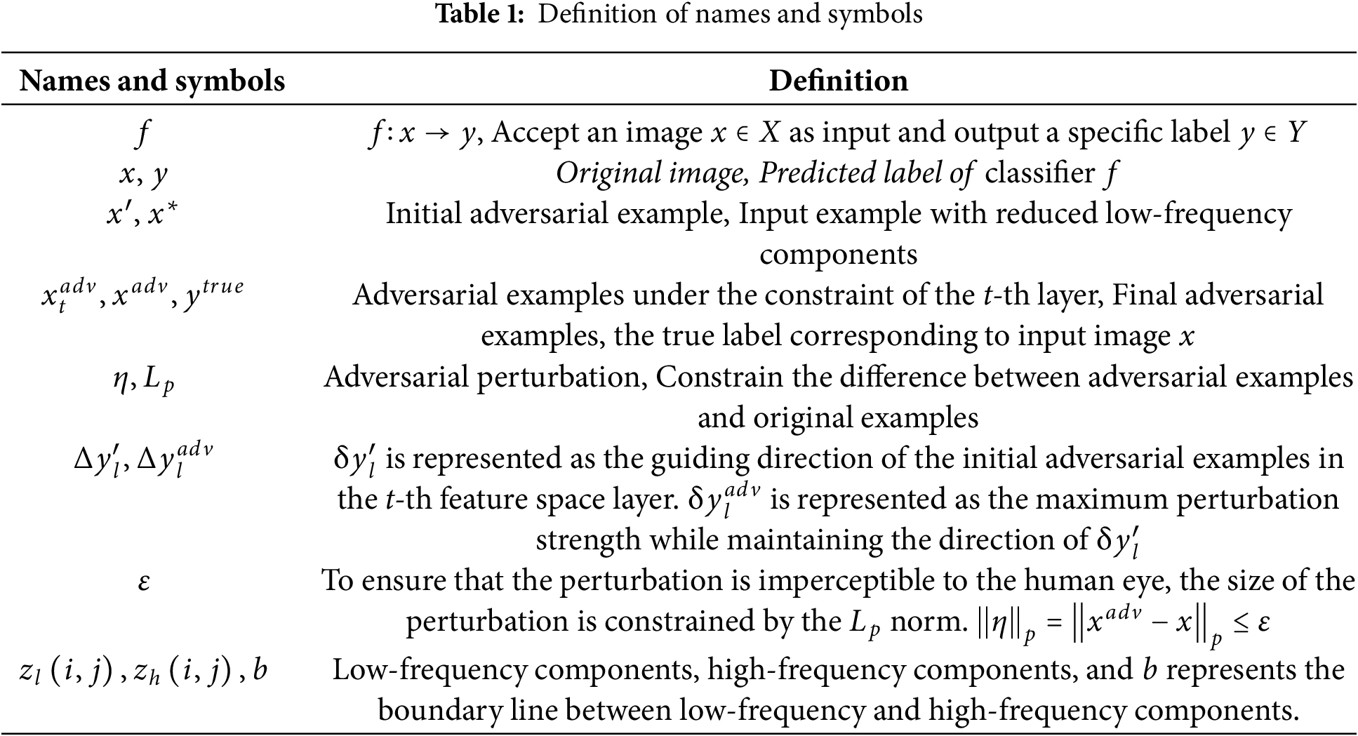
Through formal definition, it can be observed that the generation process of adversarial examples is an optimization problem, which involves finding the minimum perturbation to the model input that leads to misclassification. A list of relevant terms and their explanations is presented in Table 1.

2.2 Transfer-Based Adversarial Attack Methods

2.2.1 Momentum Iterative Fast Gradient Sign Method (MI-FGSM)

Dong et al. [20] proposed the MI-FGSM technique where the updated process of the momentum term uses the accumulated gradient , and the represents the iteration count. See Eq. (2), for dimensions where the current gradient points are in the same direction as the previous step, increases. On the other hand, for dimensions where the current gradient points are in the opposite direction as the previous step, is decreased.

(2)

2.2.2 Diverse Input Method (DIM)

Xie et al. [21] proposed a DIM to improve the transferability of adversarial examples. See Eq. (3), DIM randomly applies a set of label-preserving transformations (such as resizing, cropping and rotation) to train images and computes gradients by feeding the transformed images into the classifier.

(3)

2.2.3 Penalizing Gradient Norm (PGN)

Ge et al. [22] The PGN attack aims to guide adversarial examples towards flatter regions by constraining the norm or magnitude of the gradient. PGN is derived by optimizing Eq. (4) to achieve a flat local maximum, it can be seamlessly integrated with traditional gradient-based attack methods and input transformation-based attack methods, leveraging their strengths to further improve the adversarial transferability.

(4)

where is the penalty coefficient.

2.3 Neural Network Frequency Domain Features

This section introduces some frequency domain symbols and notations that will be used in the sequel. In digital image processing, the Discrete Cosine Transform (DCT) is often applied to transform an image from the spatial domain to the frequency domain. Moreover, and are defined, where represents the frequency spectrum of the input image and the stands for the inverse Discrete Cosine Transform.

Since the low-frequency components are in the top-left corner of the frequency spectrum , this method uses a threshold parameter to represent the boundary between the low-frequency and high-frequency components. Considering an single-channel image with , where represents the size of the image and is the set of pixel values, the low-frequency and high-frequency components can be represented as follows, see Eq. (5).

(5)

where and represent the rows and columns indices, respectively.

If the input image has multiple channels, this process is applied to each channel separately, which is represented in this paper as follows, see Eq. (6).

(6)

3  Approach

3.1 Regularized Constraint Feature Layer (RCFL)

The proposed adversarial transfer attack method based on regularization-constrained feature layers is shown in Fig. 1. This method can be divided into the following five steps:

•   Regularization constraints are added to the initial examples in the iterative attack method, the low-frequency components are removed, and input examples are generated;

•   The neural network model is attacked through the current basic transferability attack algorithm. For example, model B presented in Fig. 1 is attacked to generate the initial adversarial examples ;

•   The attacked model B is divided into different neural network feature layers. That is, the convolutional layers of the attacked model are divided;

•   Using the initial adversarial example as input, the regularization loss function is adopted to correct it in the feature layer of the attacked neural network model B. This allows for balancing the direction and intensity of the adversarial perturbation through backpropagation and seeking a better transfer direction while filtering out the high-frequency components and generating the corresponding adversarial examples after each feature layer;

•   The adversarial examples from different layers are transferred to attack other network models. Moreover, the statistical results are employed to select the optimal transfer layer. The adversarial examples from the optimal layer are finally considered as the final adversarial examples .

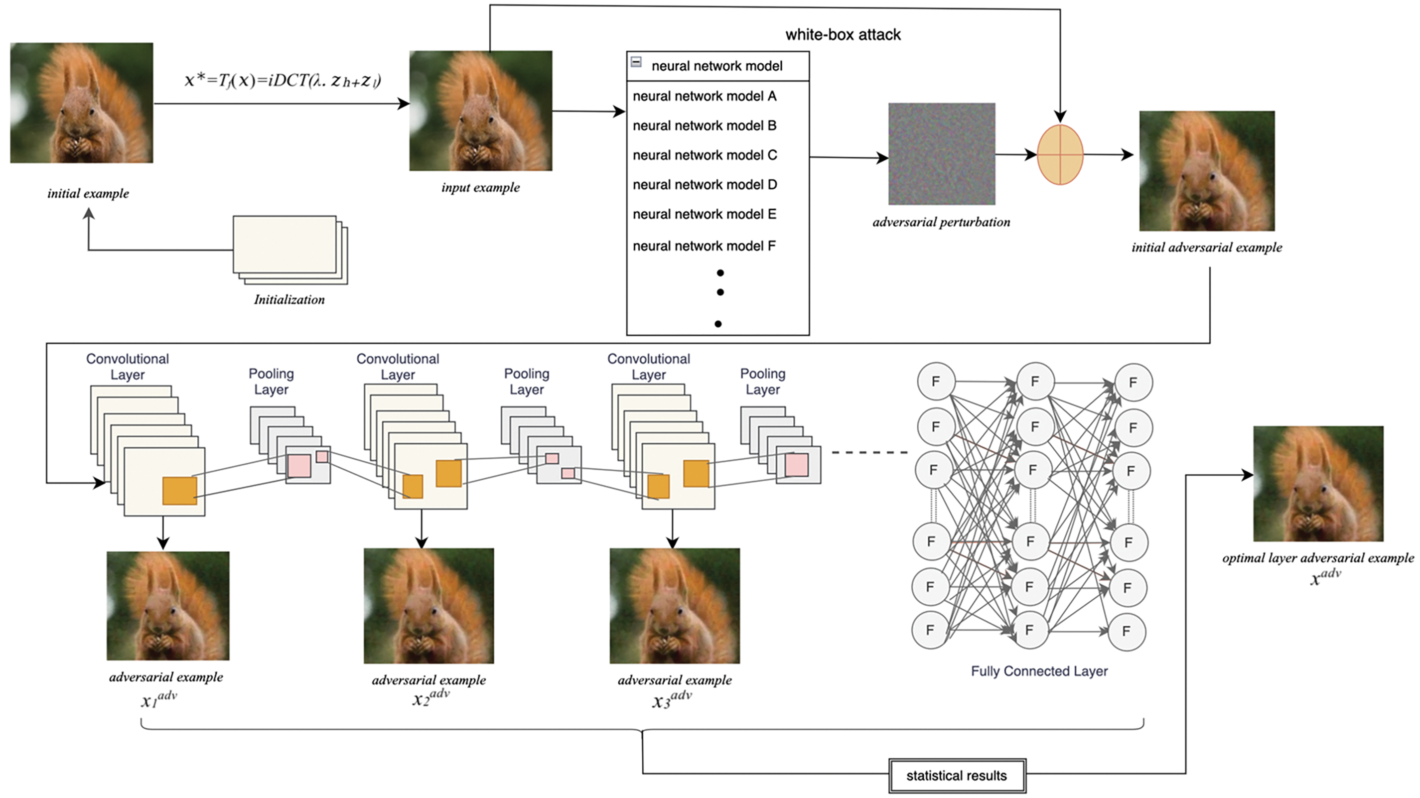
Figure 1: Adversarial examples Generation Process Diagram

3.2 Regularization Techniques

Inspired by the common regularization strategies in the training process of Deep Neural Networks (DNNs), this paper proposes a regularization-based approach to suppress the overfitting of source models to adversarial examples, thereby improving the transferability of adversarial examples. Specifically, two regularization constraints are imposed in this paper:

•   Frequency domain regularization.

•   Regularization loss function.

Firstly, we find that the CNNs exhibit differences in the low-frequency components compared to input examples. In other words, the attenuation of the low-frequency components of the input examples results in significant changes in the output of deep models. Since the changes in low-frequency components may result in changes in overall brightness, loss of detail or blurring, texture, and image contrast. Thus, even small modifications in low-frequency components can effectively perturb the decision boundaries of the model. Secondly, concerning the loss function, the implementation of a regularization loss function constraint is proposed for iterative attack methods. The aim of this approach is to reduce the high-frequency components of adversarial perturbations and minimize the differences between different adversarial perturbations, thereby reducing the impact of adversarial perturbations on transferability.

3.2.1 Frequency Domain Regularization

In the process of training DNNs, low-frequency components are firstly fit, followed by high-frequency components. However, during the fitting of the high-frequency components, the learning of the low-frequency components continues. As a result, the DNNs learn more redundant features from the low-frequency components of input examples. Therefore, a regularization term is introduced in the initial examples to reduce the low-frequency components. In this paper, a regularization constraint is constructed as an iterative attack method in the frequency domain. See Eq. (7).

(7)

where represents the attenuation factor of the low-frequency components. The examples satisfy the constraint on the initial examples . Moreover, the values of and are calculated using Eq. (6). The high-frequency component remain unchanged. Therefore, for , . The key aspect of adding the regularization constraint to the adversarial examples lies in the way of choosing an appropriate attenuation factor . A simple idea consists in setting a fixed attenuation factor for all the cases. However, to achieve better performance, during the iteration process, this method randomly selects the value of the attenuation factor within the range of (0, 1]. The case of is excluded because it is meaningless. The values of are uniformly distributed in the range of 0–1 and centered around 0.5. The random sampling strategy is adopted to obtain diversity while generating the regularization constraint. Note that this is similar to the idea of random dropout. The attenuation factor is defined as , where the latter function represents uniform sampling returning a value uniformly distributed in the range of (0, 1].

The reduction of low-frequency components can effectively perturb the decision boundary of the model, especially in instances where these components are slightly modified. Different examples have varying sensitivities to modifications in low-frequency components. Therefore, the random values can be adaptively adjusted based on the characteristics of different examples, which makes the approach more flexible in dealing with adversarial attacks. On the contrary, if is fixed, the model may become overly reliant on this value, which results in insufficient or excessive disturbances in the low-frequency components, which may affect the effectiveness of the attack. For example, if is too small, it may fail to effectively remove redundant low-frequency features, which results in low attack performance. If is too large, it may excessively remove low-frequency components, which results in decreasing the quality of the image and affects the stealthiness of the attack. This dependence can be reduced by randomly choosing the value of in the interval of (0, 1], which automatically adjusts and enhances the adaptability of the model.

3.2.2 Regularization Loss Function

This paper uses the regularization loss function to design two loss function terms. Specifically, under the constraint of the t-th layer in the neural network, Eq. (8) shows the constraint equation for the adversarial examples.

(8)

where represents the input examples after reducing the low-frequency components, is the output adversarial examples under the constraint of the t-th layer, represents the weight factor which is a constant in this study, and represent the projection loss function and the smoothness loss function that constitute the regularization loss function . The projection loss function is modelled as follows, see Eq. (9).

(9)

The projection loss function primarily calculates the projection intensity strength to ensure that the generated adversarial paradigm provides a better transfer direction and fewer high-frequency perturbation components compared with the initial adversarial examples. It is redefined that the adversarial perturbation is based on . In addition, represents the output function of the feature space layer, represents the guiding direction of the initial adversarial examples in the t-th feature space layer, and represents the maximum perturbation strength while maintaining the direction of . In other words, is the adversarial perturbation added through the regularization loss function in the t-th layer, while represents the adversarial perturbation of the initial adversarial examples in the t-th layer.

In general, simple and smooth functions tend to exhibit better generalization ability compared to complex and oscillating functions. Therefore, for the regularization term, a smoothness loss function is adopted to filter out the high-frequency components of the adversarial perturbation. This involves a convolution operation, which is similar to the application of a smoothing filter. This filter aims to make the neighboring pixels smoother. The smoothness loss function is represented as Eq. (10).

(10)

where represents the reshaped one-dimensional feature output of the t-th layer, which is generated by rearranging as the input. Moreover, denotes the smooth filtering loss function, sliding over the image and calculates the weighted sum of each pixel with its neighboring pixels. This helps reduce the differences between neighboring pixels, resulting in a smooth effect. “Pixel-wise” refers to the independent processing or calculation of each individual represents the regularization term.

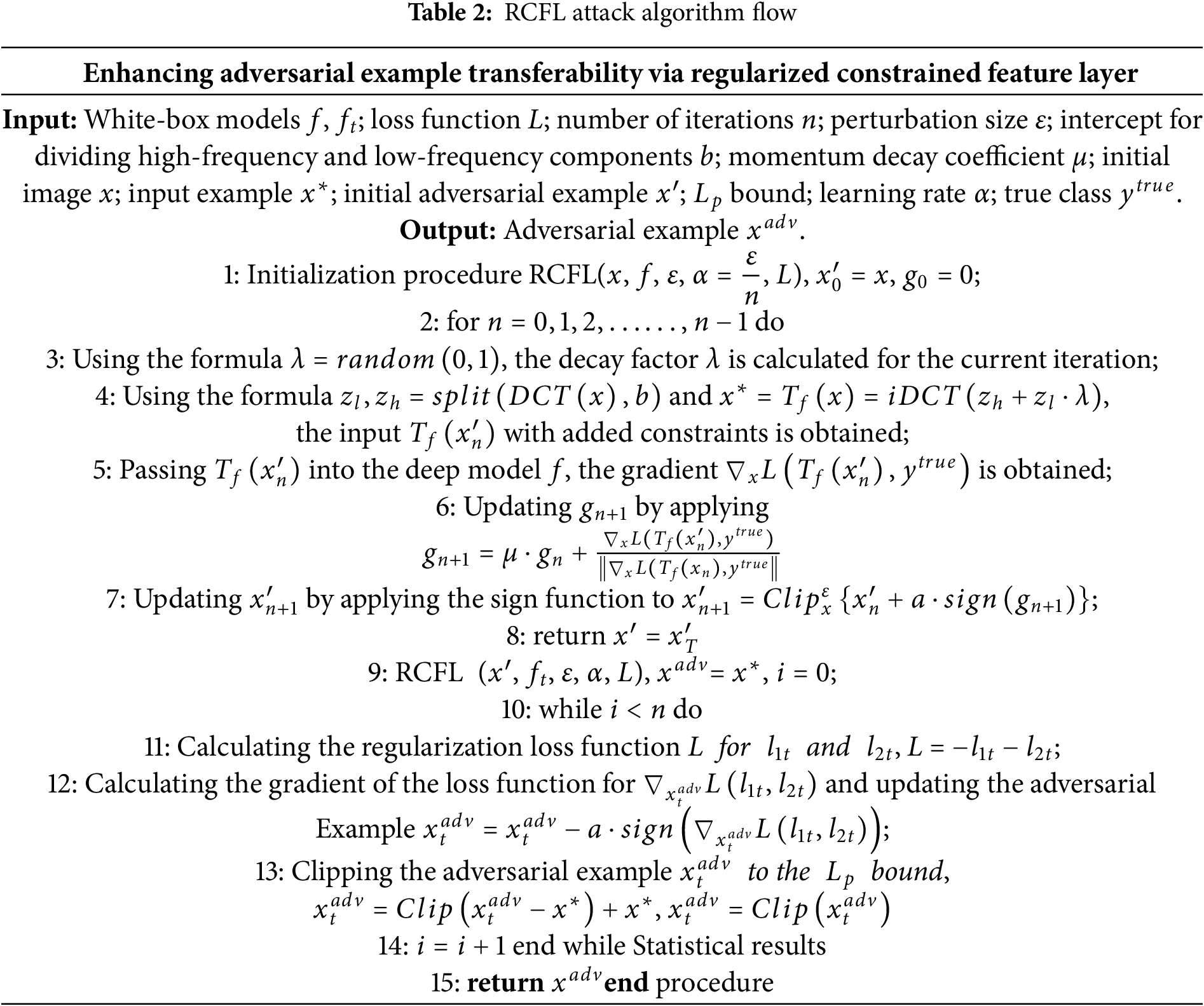
3.3 The RCFL Attack Algorithm Flow

This paper proposes an adversarial transfer attack algorithm based on regularization-constrained feature layers, as shown in Table 2. The algorithm is the final process allowing to obtain the adversarial examples based on the iterative transfer attack MI-FGSM [20], which is referred to as MIM in this paper. It can also be combined with other iterative algorithms, such as DIM [21] and PGN [22].

In addition, the differences between the adversarial examples generated by the proposed method and the original images are visually compared, the same is performed for the examples generated by traditional methods, such as the MI-FGSM algorithm. The obtained results are shown in Fig. 2. From the perspective of image perception, it can be clearly seen that the differences between the adversarial examples generated by the proposed method and the original images are much smaller than those generated by the MI-FGSM algorithm. This is due to the fact that an increase in the strength of the adversarial examples often reduces the perceptibility of the image. Therefore, while ensuring the ability to deceive classification models, the adversarial examples generated by the proposed method are clearly more realistic and closer to the real images.

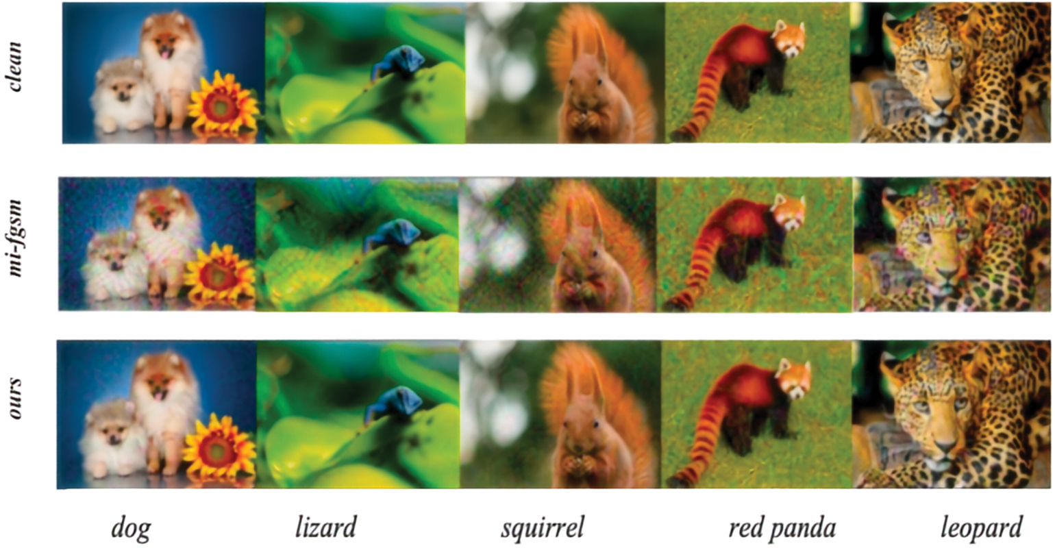
Figure 2: Clean examples (top row), adversarial examples crafted by the MI-FGSM algorithm (middle row), and adversarial examples produced by the algorithm we proposed (bottom row)

To verify the superiority of the proposed method, the limitations of the existing algorithms in the generation of adversarial examples are summarized as follows. Dong et al. [20] used a momentum term to stabilize the update direction, which is sensitive to the structure and feature representation of the target model and may get stuck in local optima, making the effective attack of different types of models difficult. Xie et al. [21] employed transformations, such as image scaling, cropping, and rotation, which may not effectively capture subtle feature differences in the images and require multiple transformations and gradient calculations for each training image. Ge et al. [22] guided the adversarial examples to move towards flatter regions by constraining the gradient norm. However, the non-linearity of the adversarial perturbations and the limitations of the gradient norm constraint may result in reducing the transferability of the adversarial examples.

On the contrary, the proposed method generates adversarial examples at the feature layer output and conducts an analysis from a unique frequency domain perspective. This approach more effectively deals with the linearization of models and generates more deceptive adversarial examples. Therefore, it effectively prevents overfitting to the substitute model, which improves the adversarial transferability. This is also proved by the experimental results shown in Tables 3 and 4 in Section 4. Referring to Fig. 3, the clean examples are recognized as “leopards” in the four NN models. The adversarial examples attacked by the MIM algorithm are successful in two out of the four targeted models, while those attacked by the proposed RCFL algorithm are successful in all the targeted models. This demonstrates that the latter is able to generate adversarial examples with better transferability.

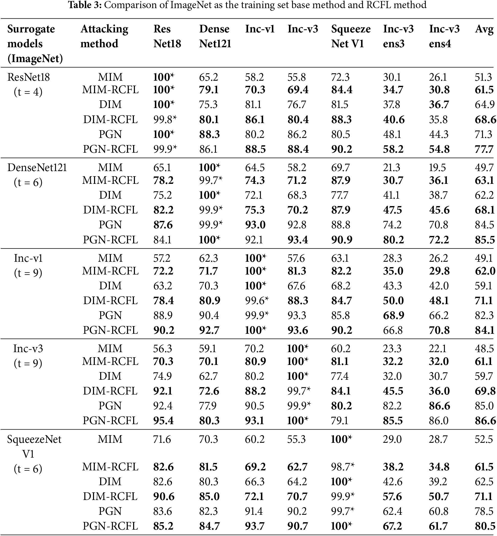
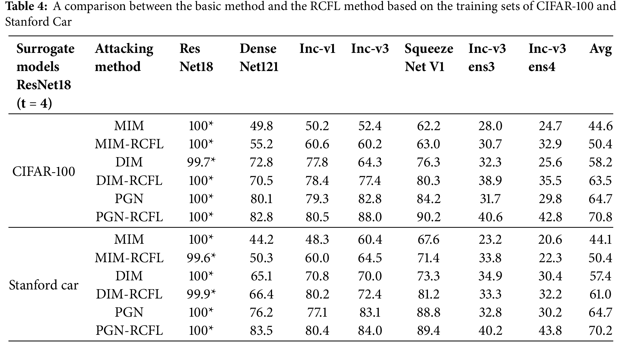
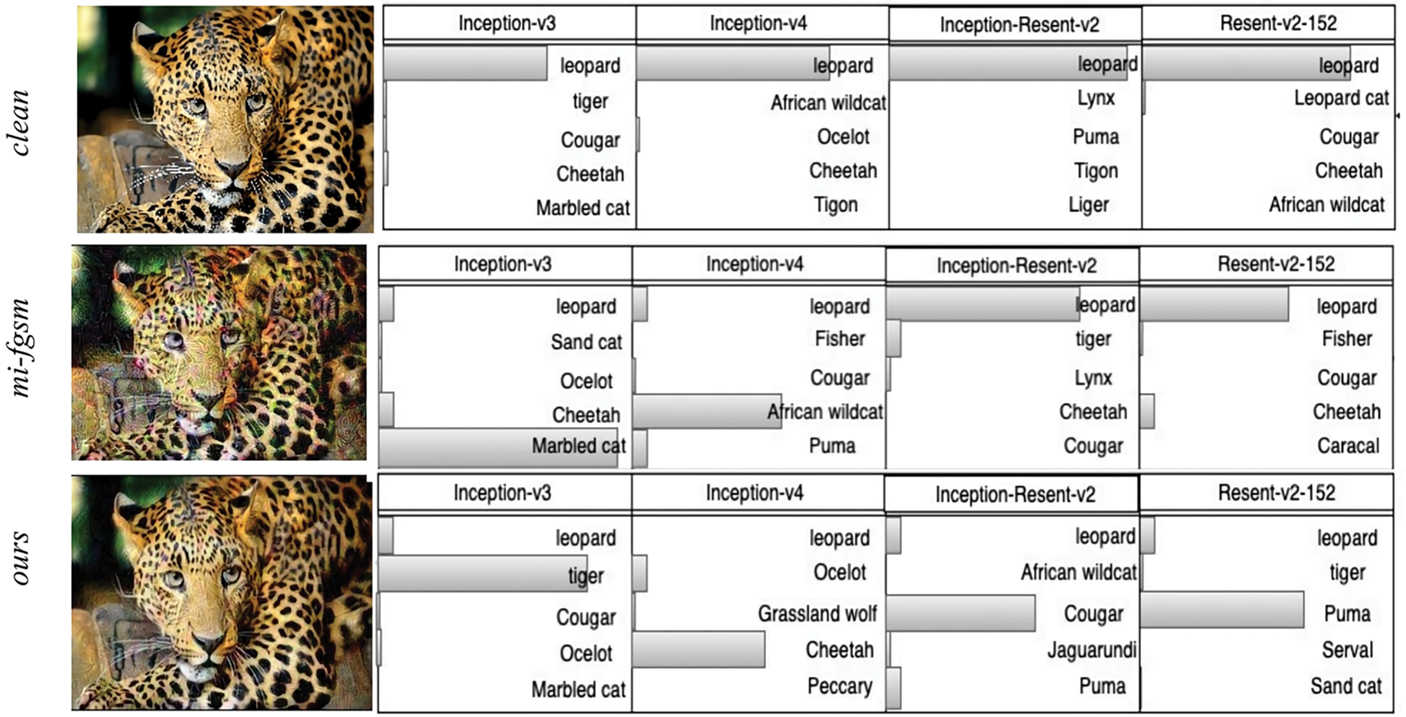
Figure 3: On the left, we have the original image at the top, the adversarial example image processed by the MI-FGSM algorithm in the middle, and the adversarial example image produced by our proposed algorithm at the bottom. On the right, the corresponding recognition results of these images by different models are displayed

4  Experiment

4.1 Experimental Setup

4.1.1 Dataset

This paper conducts experiments on three datasets: ImageNet (https://image-net.org/) (accessed on 05 January 2025), CIFAR-100 (https://www.cs.toronto.edu/~kriz/cifar.html) (accessed on 05 January 2025), and Stanford Car (https://ai.stanford.edu/~jkrause/cars/car) (accessed on 05 January 2025). ImageNet is a large-scale image dataset that contains approximately 1.2 million images, covering a wide range of different objects. Using ImageNet allows us to effectively evaluate the generality and scalability of our methods in handling large-scale, diverse image tasks, thereby reflecting their performance in complex real-world scenarios to some extent.

CIFAR-100 is a coarse-grained image classification dataset, consisting of approximately 60,000 images categorized in 100 different classes. Compared to ImageNet, CIFAR-100 has lower image resolution and simpler categories, making it suitable for studying the problem of adversarial transfer in low-resolution images. Stanford Car is a fine-grained classification dataset, Specializing in the automotive category, comprising around 16,185 images and 196 categories of cars. The fine-grained classification task places higher demands on the model’s generalization ability and robustness, and choosing the Stanford Cars dataset helps us evaluate the transfer performance of adversarial examples when facing different instances of the same category.

By selecting these three datasets, we are able to comprehensively evaluate the generation methods of adversarial examples and their transferability from different dimensions and complexities. These datasets cover tasks ranging from large-scale general image classification to fine-grained specific domain classification, making them broadly representative for comparison.

4.1.2 Network Models

To validate the transferability of the black-box attack method, this paper uses five normally trained and two adversarial-trained models. The normally trained models include ResNet18 [23], DenseNet121 [24], Inception-v1 (Inc-v1) [25], Inception-v3 (Inc-v3) [26], and SqueezeNet V1 [27]. These models are then utilized as white-box models (Surrogate models) to generate adversarial examples. As for the two adversarial trained deep models, namely ens3-adv-Inception-v3 (Inc-v3ens3) and ens4-adv-Inception-v3 (Inc-v3ens4) [28], they are applied to verify the effectiveness of the proposed method.

4.1.3 Attack Methods

We selected the classic gradient-based transfer attack method MIM, as well as more recent and powerful methods such as DIM and PGN, for comparison with the proposed attack algorithm. The proposed RCFL attack method was matched with these three methods—MIM, DIM, and PGN, and were referred to as MIM-RCFL, DIM-RCFL, and PGN-RCFL, respectively. The transferability performance of these attacks across different neural network models is then tested to verify the superiority of the proposed method.

4.1.4 Hyper-Parameter

In the case where the pixel values are in the range of 0–255, the perturbation size is set to 30. Furthermore, the attack is performed for iterations, the learning rate is set to 0.15, and the momentum decay coefficient is set to 0.5. The weight factor for the smooth loss function is set to 0.01, while the size of the used convolution kernel is set to 5 × 5. For DIM and DIM-RCFL, the probability of the input random transformations is set to 0.5. Note that the other hyper-parameters are set according to the specifications in their respective published work. In this paper, the uniform sampling random set (0.001, 1) is used to avoid obtaining a null value. Finally, this function returns a value uniformly sampled in the range of 0.001-1.

4.2 Experimental Results

4.2.1 Optimal Transfer Layer of the Model

The basic idea for identifying the optimal transfer layer of the statistical model is to use different neural network models sequentially as surrogate models. The RCFL attack algorithm is employed to generate a set of adversarial examples for each surrogate model. These adversarial examples are then used to attack other target models, excluding the surrogate model, and the transfer attack success rate is computed for each layer. We selected the layer with the highest success rate of transfer attacks against the target model as the final confrontation example and identified as the optimal transfer feature layer of the surrogate model. For example, if Inception-v1 (Inc-v1) is used as the surrogate model, the RCFL attack algorithm generates adversarial examples at each layer, forming a set of adversarial examples . These examples are then sequentially used to attack ResNet18, DenseNet121, Inception-v3 (Inc-v3), SqueezeNet V1, ens3-adv-Inception-v3 (Inc-v3ens3), and ens4-adv-Inception-v3 (Inc-v3ens4), obtaining the transfer attack success rate for each layer. The layer with the highest average transfer attack success rate is determined to be the optimal transfer feature layer of the neural network model. As shown in Fig. 4a,b, when Inception-v1 is used as the surrogate model, the layer is identified as the optimal transfer layer.

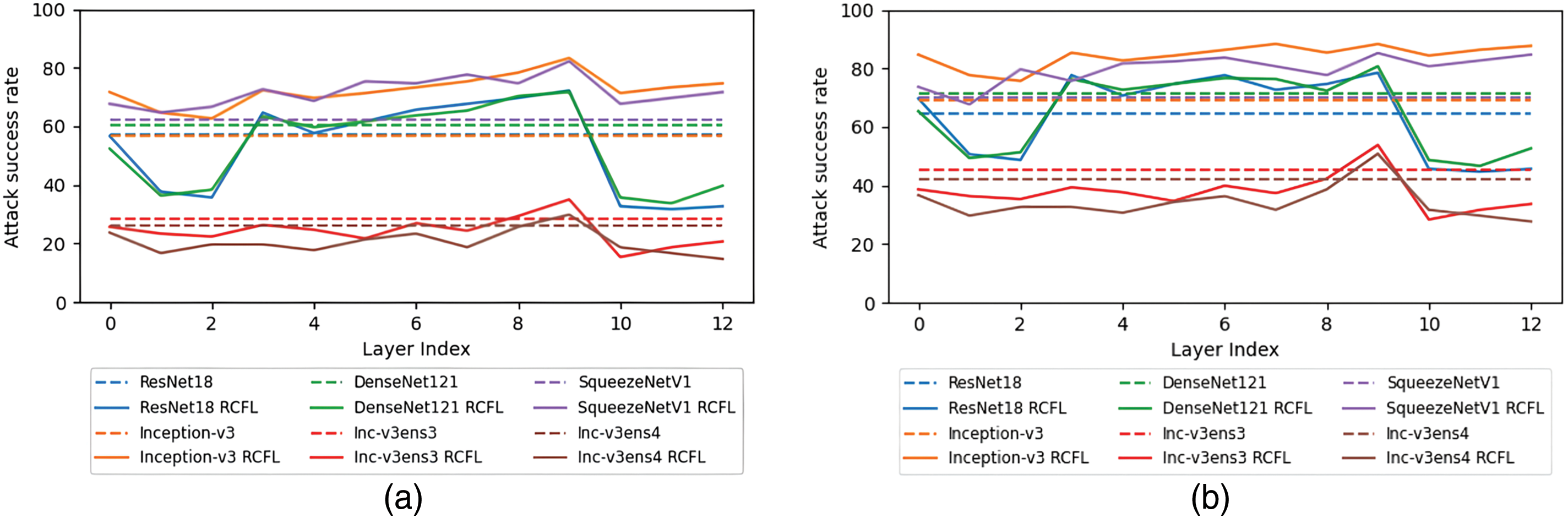
Figure 4: The results of two sets of experiments, which used the ImageNet dataset. The horizontal axis represents the number of different feature layers of the surrogate model Inception-v1, while the vertical axis represents the transfer attack success rate of the adversarial examples generated at these layers on the target model. The dashed line indicates that the model’s output is not layered, and the solid line is the opposite. (a) shows the results using the MIM algorithm as the basis for RCFL, and (b) shows the results using the DIM algorithm as the basis for RCFL

The experimental results show that different basic algorithms have no effect on the selection of the optimal feature layer of the model. Therefore, to determine the optimal layer for the other four models, we uniformly use ImageNet as the dataset and the MIM transfer attack algorithm as the basis for our RCFL method. The experimental results for the optimal transfer layers of the four standard-trained models—ResNet18, DenseNet121, Inception-v3, and SqueezeNet V1—are shown in Fig. 5a–d. the optimal layer for ResNet18 is , for DenseNet121 is for Inception-v3 is , and for SqueezeNet V1 is .

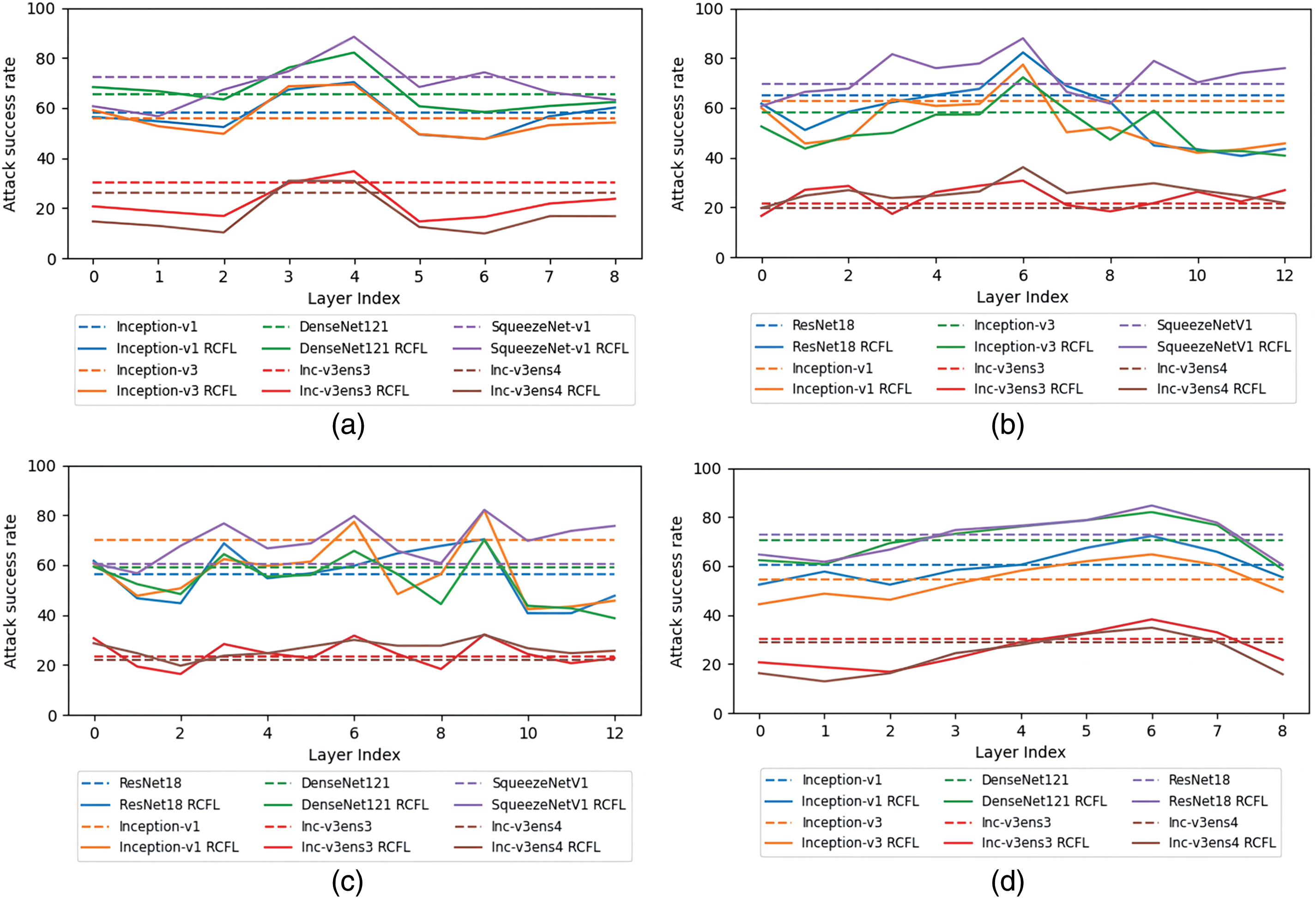
Figure 5: The optimal transfer layer of different models. The horizontal axis in the figure represents the number of layers in the feature layer of the surrogate model, and the vertical axis indicates the transfer attack success rate of adversarial examples generated from different layers on the target model. The dashed line indicates that the model’s output is not layered, and the solid line is the opposite. (a) shows the surrogate model using ResNet18. (b) shows the surrogate model using DenseNet121. (c) shows the surrogate model using Inception-v3. (d) shows the surrogate model using SqueezeNet V1

4.2.2 Comparison between the Transferability of the Adversarial Examples

To optimal feature layers for the five standard-trained models are determined based on the aforementioned experiment results. The surrogate models and the attacked black-box models are then trained using the ImageNet, CIFAR-100, and Stanford Car datasets. Adversarial examples are first generated on the optimal feature layers of the five standard training models. They are then used to attack all the five standard training models and two adversarial training models in the same training set, in order to measure their attack success rates. MIM, DIM, and PGN are used as the basis transfer attack algorithms for RCFL. A comparison between the results of MIM and MIM-RCFL, DIM and DIM-RCFL, and PGN and PGN-RCFL on different training sets is shown in Tables 3 and 4, Note that the results presented in Table 3 are obtained when using the ImageNet dataset, with surrogate models including ResNet18, DenseNet121, Inception-v1, Inception-v3, and SqueezeNet v1. The first column indicates adversarial examples generated by different surrogate models, * denotes white-box attack results, and the last column shows the average attack success rate for the six black-box models. The results presented in Table 4 are obtained when using the CIFAR-100 and Stanford Car datasets, with ResNet18 as the surrogate model. The first column indicates the use of different datasets, * also denotes white-box attack results, and the last column shows the average attack success rate for the other six black-box models.

It can be observed that the proposed RCFL attack method significantly improves the attack success rate under black-box attack settings for standard-trained and adversarially trained models, while also ensuring a high white-box attack success rate. In terms of numerical values, when using ImageNet as the training set, the proposed method outperforms MIM, DIM, and PGN by averages of 11.6%, 8.0%, and 2.6%, respectively. When using CIFAR-100 as the training set, the proposed method outperforms MIM, DIM, and PGN by averages of 5.8%, 5.3%, and 6.1%, respectively. When using Stanford Car as the training set, the proposed method outperforms MIM, DIM, and PGN by averages of 6.3%, 3.6%, and 5.5%, respectively. This demonstrates that the adversarial examples generated by the proposed regularized constrained feature layer method have better transferability.

4.2.3 Ablation Experiment

(1) Constraint factor

In this section, ablation experiments are conducted to study the impact of the proposed constraint factor on transferability and to verify that the random strategy of outperforms that of a fixed value. A normally trained model is then used to generate adversarial examples and black-box attack tests are conducted on four other normally trained models and two adversarially trained models. Afterward, the black-box attack results obtained by these six models are averaged and compared with baseline methods (e.g., MIM, DIM, and PGN) and the proposed complete method using the random selection decay factor (e.g., MIM-RCFL, DIM-RCFL, and PGN-RCFL). The obtained results are shown in Fig. 6a–d.

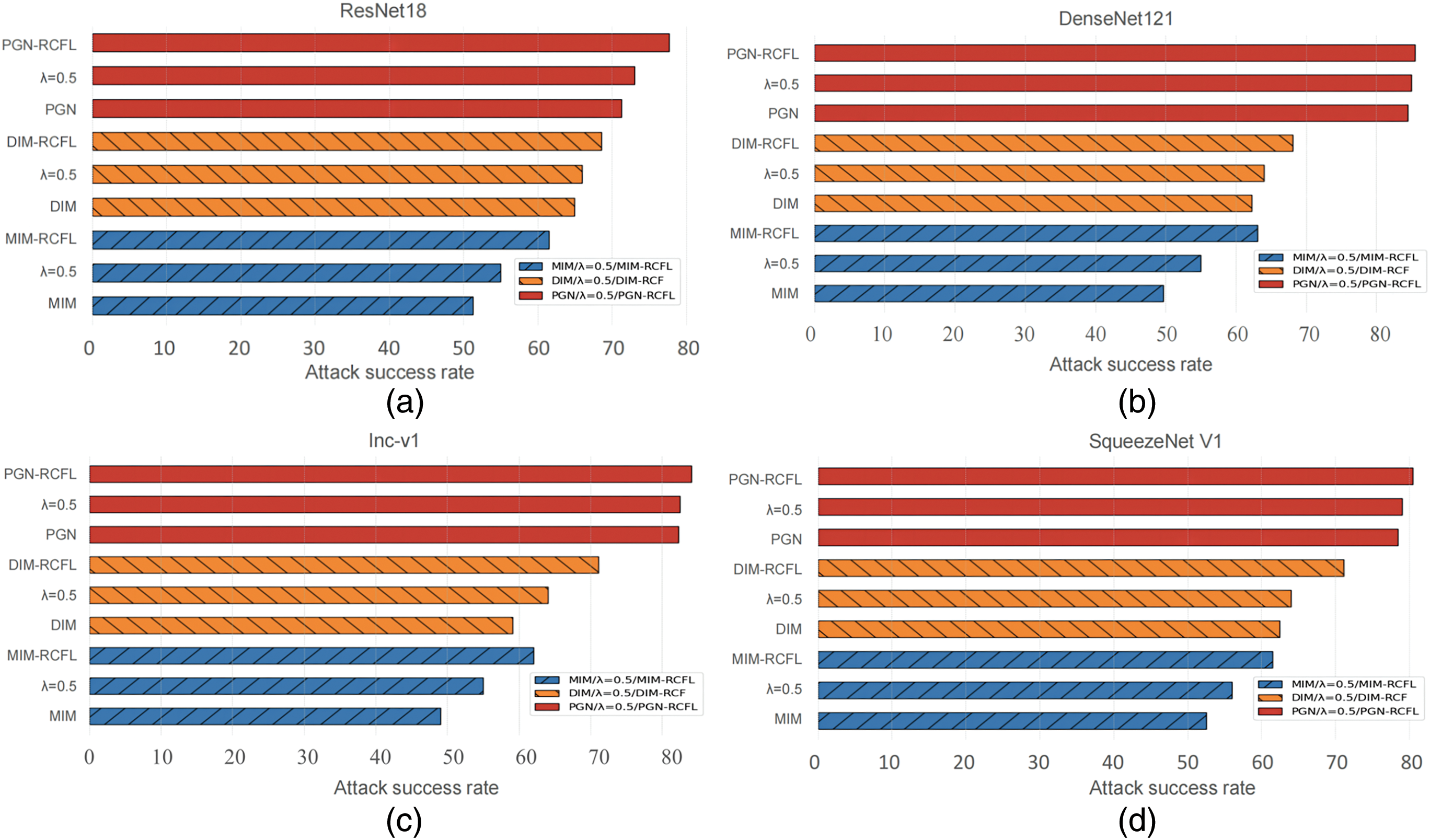
Figure 6: The performance comparison of different attenuation factors. The x-axis represents the average attack success rate against the six black-box models, while the y-axis represents the different attack methods. indicates the experimental results using a fixed decay factor. (a) shows the surrogate model using ResNet18. (b) shows the surrogate model using DenseNet121. (c) shows the surrogate model using Inception-v1. (d) shows the surrogate model using SqueezeNet V1

It can be seen that the adversarial examples generated by the fixed decay factor method still outperform the baseline method, However, when the fixed decay factor strategy is replaced with the proposed random sampling strategy, the transfer performance of the generated adversarial examples is significantly increased, which is consistent with the analysis presented in Section 3.2.1.

(2) Impact of the regularization on the transferability

This paper systematically analyzes the impact of regularization techniques on the transferability of adversarial examples. When the frequency domain regularization (“RCFL w/o FDR”) or the regularization loss function (“RCFL w/o RLF”) is removed, the success rate of the adversarial attacks significantly decreases, as shown in Fig. 7a. This indicates that the frequency domain regularization and the regularization loss function play a key role in enhancing the adversarial transferability. Although the proposed method acquires a small additional computational overhead (Fig. 7c), the latter is reasonable considering its significant impact on the improvement of the transferability of the adversarial examples.

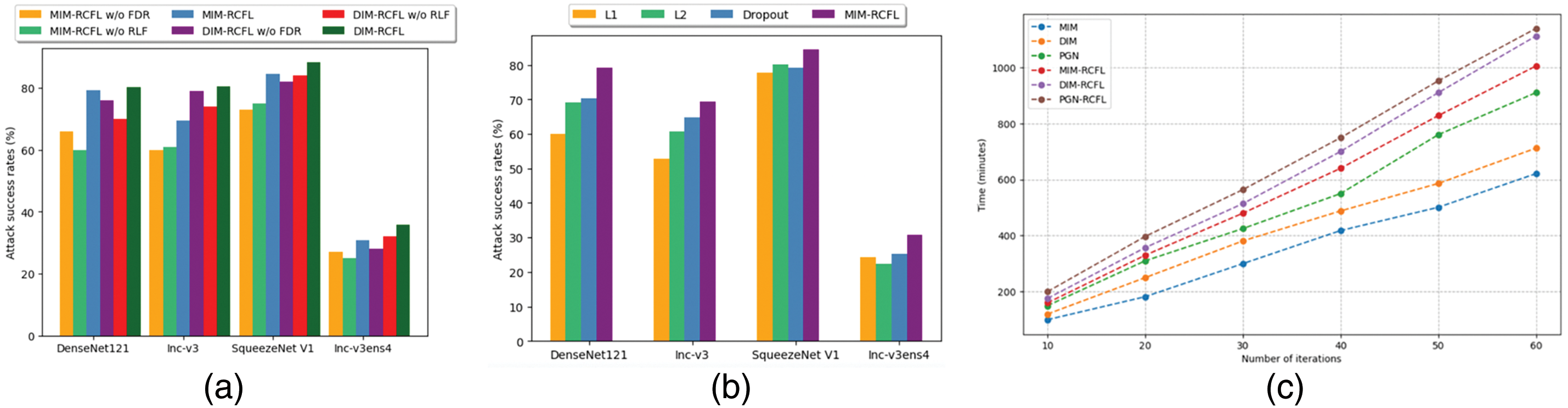
Figure 7: Comparison of attack success rates and time consumption of different attack and regularization methods. (a) shows the attack success rates of different algorithms on different models in the ImageNet dataset. (b) shows the attack success rates of different regularization methods on different models in the ImageNet dataset. (c) shows the time consumption of different methods at different iteration counts on the CIFAR-100 dataset

(3) Comparison between different regularization strategies

This section presents a comparison between regularization strategies allowing us to study their impact on the adversarial transferability of the model. In the conducted experiments. The , , and Dropout are used as regularization methods. The obtained results shown in Fig. 7b, compared with the proposed RCFL method, the success rate of adversarial attacks decreased after applying the aforementioned regularization methods. This indicates that the frequency domain regularization and regularization loss function underlying the RCFL method play a crucial role in enhancing the adversarial transferability of the model.

(4) Time performance analysis of the RCFL method

In the proposed method, the regularization mechanism requires additional processing of the feature space, which increases the computational load during iterations. To quantify this increased computational burden, the running time required to generate adversarial examples for different methods using the CIFAR-100 and ResNet18 models under the same hardware environment with 60 iterations, is recorded and compared with the MIM, DIM, and PGN traditional methods that do not introduce regularization. The experimental results are shown in Fig. 7c. It can be seen that the running time of the RCFL variants (i.e., MIM-RCFL, DIM-RCFL, and PGN-RCFL) is higher than their corresponding baseline methods, which demonstrates that the introduced regularization computation increases the running time.

However, the additional computational overhead introduced by the RCFL method is still within an acceptable range, and it has a small impact on practical applications. This demonstrates that, although the computational load is increased, the RCFL method has significant advantages in enhancing the transferability and increasing the attack effectiveness of adversarial examples. Therefore, this study believes that the balance between the performance improvement of the RCFL method and the computational overhead is reasonable, and the proposed method can be effectively used.

(5) Logits analysis of adversarial example generation

The outputs of the model during the generation of adversarial examples are studied to further demonstrate that the proposed method can enhance the transferability of the adversarial examples. The output logarithmic values for all 10 iterations are recorded, the maximum logarithmic value for each image is labeled, and those of the 1200 validation images are then averaged. The obtained results are shown in Fig. 8a,b.

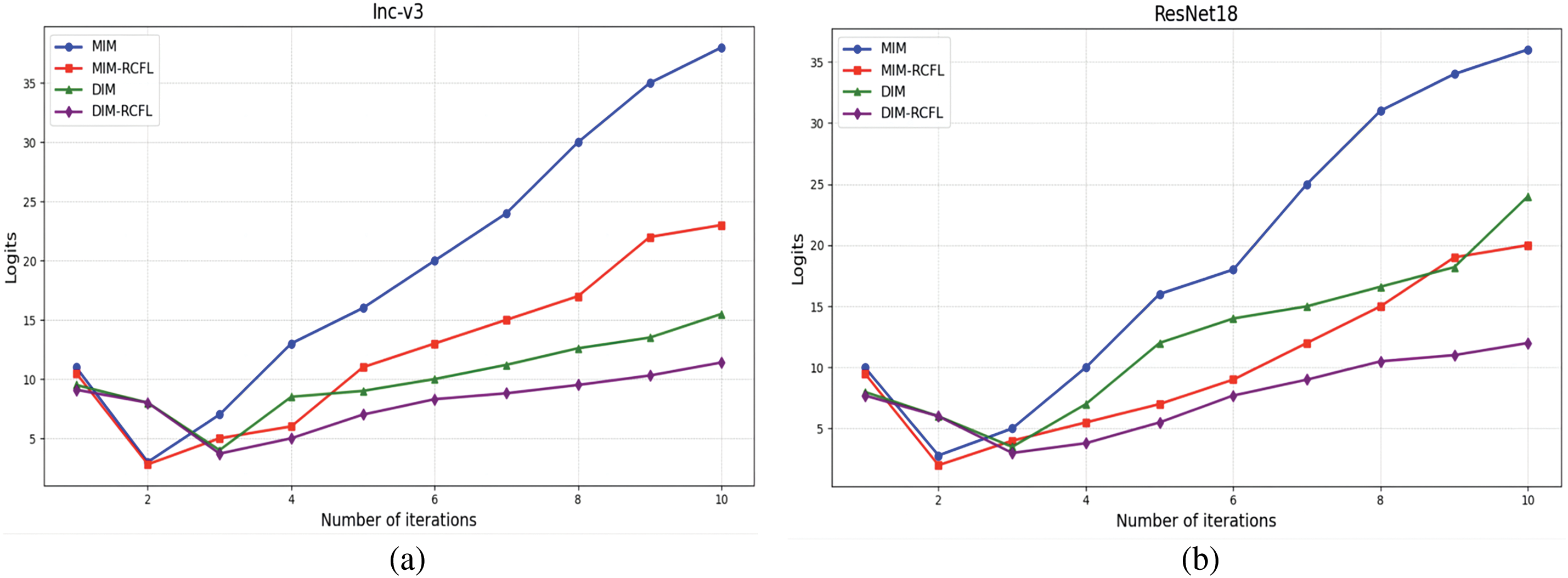
Figure 8: The iterative variation figure of the maximum logits mean of the model under different algorithms (MIM and DIM, as well as MIM-RCFL and DIM-RCFL). (a) The change in the maximum logits mean of Inception-v3. (b) The change in the maximum logits mean of ResNet18

It can be seen that the performances of the same model for various algorithms are different. This is due to the fact that the MIM, DIM, and proposed RCFL, have different characteristics when generating adversarial perturbations. The MIM and DIM methods focus on specific adversarial perturbation generation, while the RCFL method is able to achieve more balanced prediction outputs by introducing regularization constraints. In addition, the performances of different models for the same algorithm are inconsistent. This is mainly due to the different internal structures and parameters of ResNet18 and Inception-v3, which affect the generation and transferability of the adversarial examples.

Specifically, the results in Fig. 8a,b show that the largest logits in the predicted categories first decrease rapidly at the beginning, yielding at this point the model cannot correctly categorize the input images with high confidence, i.e., the adversarial attack has achieved good results.

However, as the iterations progressed, the logits values started to increase, this indicates that adversarial examples can make the model misclassify with high confidence, which demonstrates that overfitting occurs in the surrogate model, and the adversarial examples are difficult to transfer to other black-box models. The proposed regularization constraint method effectively solves this problem by limiting the maximum logits of the predicted categories within a lower range. This restriction makes the predictions of the white-box model more balanced in all the categories and prevents the generated adversarial examples from overfitting the surrogate model. This leads to a better transfer of the adversarial examples to other black-box models.

5  Conclusion

This paper proposed a method for generating adversarial examples based on the RCFL technique. This method applies frequency domain and loss function regularizations. The frequency domain regularization aims to suppress low-frequency components. The loss function regularization plays a crucial role in attenuating the high-frequency components within these adversarial perturbations and finding the optimal transfer direction. The proposed approach for the generation of adversarial examples at the feature layer output allows the RCFL method to modify the adversarial examples produced by classical transfer attack algorithms using the regularization loss function. This method achieves better transferability towards black-box models. Extensive experiments are then conducted on the ImageNet, CIFAR-100, and Stanford Car datasets to demonstrate the high effectiveness of the proposed method in generating transferable adversarial examples. Although the proposed method is effective, it requires a higher computational load compared with traditional methods. In future work, the proposed algorithms will be optimized to reduce the resource consumption. Furthermore, the scope of this study will be expanded from images to text and audio content in order to tackle more diverse application scenarios.

Acknowledgement: We are grateful to our families and friends for their unwavering understanding and encouragement.

Funding Statement: This work was supported by the Intelligent Policing Key Laboratory of Sichuan Province (No. ZNJW2022KFZD002), This work was supported by the Scientific and Technological Research Program of Chongqing Municipal Education Commission (Grant Nos. KJQN202302403, KJQN202303111).

Author Contributions: The authors confirm contribution to the paper as follows: study conception and design: Xiaoyin Yi, Long Chen; data collection: Qian Huang; analysis and interpretation of results: Jiacheng Huang, Xiaoyin Yi; draft manuscript preparation: Ning Yu, Xiaoyin Yi. All authors reviewed the results and approved the final version of the manuscript.

Availability of Data and Materials: Not applicable.

Ethics Approval: Not applicable.

Conflicts of Interest: The authors declare no conflicts of interest to report regarding the present study.

References

1. Liu J, Jin Y. A comprehensive survey of robust deep learning in computer vision. J Autom Intell. 2023;2(4):175–95. doi:10.1016/j.jai.2023.10.002. [Google Scholar] [CrossRef]

2. Alawida M, Mejri S, Mehmood A, Chikhaoui B, Abiodun OI. A comprehensive study of ChatGPT: advancements, limitations, and ethical considerations in natural language processing and cybersecurity. Information. 2023;14(8):462. doi:10.3390/info14080462. [Google Scholar] [CrossRef]

3. Jeon J, Lee S, Choi S. A systematic review of research on speech-recognition chatbots for language learning: implications for future directions in the era of large language models. Interact Learn Environ. 2024;32(8):4613–31. doi:10.1080/10494820.2023.2204343. [Google Scholar] [CrossRef]

4. Zhao Y, Lv WY, Xu SL, Wei JM, Wang GZ, Dang QQ, et al. DETRs beat YOLOs on real-time object detection. In: Proceedings of the 41st Meeting of the IEEE/CVF Conference on Computer Vision and Pattern Recognition; 2024 Jun 17–21; 2024; Seattle, WA, USA: IEEE. p. 16965–74. [Google Scholar]

5. Chakraborty A, Alam M, Dey V, Chattopadhyay A, Mukhopadhyay D. A survey on adversarial attacks and defences. CAAI Trans Intell Technol. 2021;6(1):25–45. doi:10.1049/cit2.12028. [Google Scholar] [CrossRef]

6. Wang XS, He XR, Wang JD, He K. Admix: enhancing the transferability of adversarial attacks. In: Proceedings of the 18th Meeting of the IEEE/CVF International Conference on Computer Vision; 2021 Oct 11–17; 2021; Montreal, QC, Canada: IEEE. p. 16158–67. [Google Scholar]

7. Ma WS, Li YD, Jia XF, Xu W. Transferable adversarial attack for both vision transformers and convolutional networks via momentum integrated gradients. In: Proceedings of the 19th Meeting of the IEEE/CVF International Conference on Computer Vision; 2023 Oct 2–6; 2023; Paris, France: IEEE. p. 4630–9. [Google Scholar]

8. Wu T, Luo T, Wunsch DC. GNP attack: transferable adversarial examples via gradient norm penalty. In: Proceedings of the 8th Meeting of the IEEE International Conference on Image Processing; 2023 Jul 8–10; 2023; Wuxi, China: IEEE. p. 3110–4. [Google Scholar]

9. Wang X, Zhang Z, Zhang J. Structure invariant transformation for better adversarial transferability. In: Proceedings of the 19th Meeting of the IEEE/CVF International Conference on Computer Vision; 2023 Oct 2–6; 2023; Paris, France: IEEE. p. 4607–19. [Google Scholar]

10. Wu SB, Tan YA, Wang YJ, Ma RN, Ma WC, Li YZ. Towards transferable adversarial attacks with centralized perturbation. In: Proceedings of the 38th Meeting of the AAAI Conference on Artificial Intelligence; 2024 Feb 20–27; 2024; British Columbia: AAAI. p. 6109–16. [Google Scholar]

11. Chen B, Yin JL, Chen SK, Chen BH, Liu XM. An adaptive model ensemble adversarial attack for boosting adversarial transferability. In: Proceedings of the 19th Meeting of the IEEE/CVF International Conference on Computer Vision; 2023 Oct 2–6; 2023; Paris, France: IEEE. p. 4489–98. [Google Scholar]

12. Gubri M, Cordy M, Papadakis M, Traon YL, Sen K. Lgv: boosting adversarial example transferability from large geometric vicinity. In: Proceedings of the 17th Meeting of the European Conference on Computer Vision; 2022 Oct 23–27; 2022; Tel Aviv, Israel: Springer. p. 603–18. [Google Scholar]

13. Li QZ, Guo YW, Zuo WM, Chen H. Improving adversarial transferability via intermediate-level perturbation decay. Advances in neural information processing systems. In: Proceedings of the 37th Conference on Neural Information Processing Systems; 2023 Dec 10–16; 2023; Red Hook, NY, USA: Curran Associates Inc. p. 1–13. [Google Scholar]

14. Qin Y, Xiong Y, Yi J, Hsieh CJ. Training meta-surrogate model for transferable adversarial attack. In: Proceedings of the 37th Meeting of the AAAI Conference on Artificial Intelligence; 2023 Feb 7–14; 2023; Washington, DC, USA: AAAI. p. 9516–24. [Google Scholar]

15. Zhang JP, Huang YZ, Wu WB, Lyu MR. Transferable adversarial attacks on vision transformers with token gradient regularization. In: Proceedings of the 40th Meeting of the IEEE/CVF Conference on Computer Vision and Pattern Recognition; 2023 Jun 18–22; 2023; Vancouver, Canada: IEEE. p. 16415–24. [Google Scholar]

16. Zhu Y, Chen Y, Li X, Chen KJ, He Y, Tian X, et al. Toward understanding and boosting adversarial transferability from a distribution perspective. IEEE Trans Image Process. 2022;31(24):6487–501. doi:10.1109/TIP.2022.3211736. [Google Scholar] [PubMed] [CrossRef]

17. Huber P, Calatroni A, Rumsch A, Paice A. Review on deep neural networks applied to low-frequency nilm. Energies. 2021;14(9):2390. doi:10.3390/en14092390. [Google Scholar] [CrossRef]

18. Wang Y, Hong W, Zhang X, Zhang Q, Gu CH. Boosting transferability of adversarial samples via saliency distribution and frequency domain enhancement. Knowl Based Syst. 2024;300(6):112152. doi:10.1016/j.knosys.2024.112152. [Google Scholar] [CrossRef]

19. Kurakin A, Goodfellow IJ, Bengio S. Adversarial examples in the physical world. In: Artificial intelligence safety and security. Boca Raton: Chapman and Hall/CRC; 2018. p. 99–112. [Google Scholar]

20. Dong YP, Liao FZ, Pang TY, Su H, Zhu J, Hu XL, et al. Boosting adversarial attacks with momentum. In: Proceedings of the 35th Meeting of the IEEE Conference on Computer Vision and Pattern Recognition; 2018 Jun 18–22; 2018; Salt Lake City, UT, USA: IEEE. p. 9185–93. [Google Scholar]

21. Xie C, Zhang Z, Zhou Y, Bai S, Wang J, Ren Z, et al. Improving transferability of adversarial examples with input diversity. In: Proceedings of the 36th Meeting of the IEEE/CVF Conference on Computer Vision and Pattern Recognition; 2019 Jun 15–20; 2019; Long Beach, CA, USA: IEEE. p. 2730–9. [Google Scholar]

22. Ge ZJ, Liu HY, W. XS, Shang FH, Liu YY. Boosting adversarial transferability by achieving flat local maxima. Advances in neural information processing systems. In: Proceedings of the 37th Conference on Neural Information Processing Systems; 2023 Dec 10–16; 2023; Red Hook, NY, USA: Curran Associates Inc. p. 70141–61. [Google Scholar]

23. He KM, Zhang XY, Ren SQ, Sun J. Deep residual learning for image recognition. In: Proceedings of the 33rd Meeting of the IEEE Conference on Computer Vision and Pattern Recognition; 2016 Jun 27–30; 2016; Las Vegas, NV, USA: IEEE. p. 770–8. [Google Scholar]

24. Huang G, Liu Z, Van Der Maaten L, Weinberger KQ. Densely connected convolutional networks. In: Proceedings of the 34th Meeting of the IEEE Conference on Computer Vision and Pattern Recognition; 2017 Jul 21–26; 2017; Honolulu, HI, USA: IEEE. p. 4700–8. [Google Scholar]

25. Szegedy C, Liu W, Jia YQ, Sermanet P, Reed S, Anguelov D, et al. Going deeper with convolutions. In: Proceedings of the 32nd Meeting of the IEEE Conference on Computer Vision and Pattern Recognition; 2015 Jun 7–12; 2015; Boston, MA, USA: IEEE. p. 1–9. [Google Scholar]

26. Szegedy C, Vanhoucke V, Ioffe S, Shlens J, Wojna Z. Rethinking the inception architecture for computer vision. In: Proceedings of the 33rd Meeting of the IEEE Conference on Computer Vision and Pattern Recognition; 2016 Jun 27–30; 2016; Las Vegas, NV, USA: IEEE. p. 2818–26. [Google Scholar]

27. Iandola FN. SqueezeNet: AlexNet-level accuracy with 50x fewer parameters and <0.5 MB model size. arXiv:1602.07360. 2016. [Google Scholar]

28. Tramèr F, Kurakin A, Papernot N, Goodfellow I, Boneh D, McDaniel P. Ensemble adversarial training: attacks and defenses. arXiv:1705.07204. 2017. [Google Scholar]