A Global-Local Parallel Dual-Branch Deep Learning Model with Attention-Enhanced Feature Fusion for Brain Tumor MRI Classification

1  Introduction

The brain, as a crucial organ, controls central nervous system functions, and abnormal cell growth can result in tumors [1,2]. Brain tumors are the most common primary tumors of the central nervous system [3]. They mainly include meningiomas, gliomas, and pituitary tumors, each of which requiring different treatment approaches. Brain tumor classification can be based on their microscopic structure and molecular characteristics [4]. Timely and accurate classification and diagnosis of brain tumors are critical for patient prognosis, as they assist in guiding treatment decisions and thereby improving therapeutic outcomes [5].

Medical imaging technologies, particularly MRI, play a significant role in the detection of brain tumors [6]. MRI provides exceptional soft tissue contrast, enabling more precise detection of moderate infiltration or damage to parenchymal structures. Additionally, MRI offers detailed images based on morphological and textural information, providing higher detection accuracy compared to computed tomography images [7]. However, manually assessing MRI scans poses significant challenges for radiologists, and the integration of artificial intelligence methods in radiology can substantially enhance diagnostic capabilities [8]. Consequently, to alleviate the workload of clinicians and improve diagnostic accuracy, current research is increasingly focused on developing automated AI systems.

Recent developments in machine learning have significantly driven the development of AI-based medical image analysis systems [9]. In particular, CNNs have been extensively applied to medical image classification [10,11] and segmentation [12,13] tasks. CNNs are capable of efficiently extracting features directly from raw brain tumor images [14], achieving remarkable results in tumor detection and classification. However, despite numerous studies applying deep learning methods to brain tumor classification, existing models still face a major challenge: balancing the extraction of global contextual information with local feature details, especially in ensuring that small tumor regions are not overlooked. The current models, when using whole-brain images as input, often struggle to sufficiently capture the fine details of small tumor boundaries and textures.

In this context, the aim of this study is to propose a novel approach to brain tumor classification that addresses the challenges of effectively integrating global contextual features and fine-grained local tumor features, thus improving classification accuracy and robustness. The main focus of this research is the introduction of an innovative dual-branch feature fusion architecture. The global branch utilizes a ResNet50 model enhanced with a multi-head self-attention mechanism (MHSA) to capture global contextual information from the entire image, recognizing the overall shape, position, and relationship of the tumor with surrounding tissues. The local branch, on the other hand, uses VGG16 to focus on the tumor region, capturing the texture, boundaries, and internal structure of the tumor. Through this approach, our model effectively integrates both global and local features, providing a more precise and comprehensive tumor feature representation, thus enhancing classification performance, particularly in the detection of small tumor regions.

Furthermore, to achieve efficient feature fusion, we designed an Attention-enhanced Feature Fusion Module (AFFM) that incorporates a Feature Selection Module (FSM) and an Improved Efficient Channel Attention (IECA). Additionally, to resolve the issue of sample imbalance in the brain tumor dataset, we introduced a Category Attention Block (CAB) to improve the recognition of minority classes. Ablation experiments and performance comparisons on a public dataset containing three types of brain tumors validated the effectiveness of the proposed method, while five-fold cross-validation further demonstrated its stability and generalization ability. The main contributions of this paper are as follows:

1.    Enhanced ResNet50 with MHSA: To enhance the ability of the ResNet50 model to extract global features while reducing unnecessary computational overhead, the final 3 × 3 convolutional layers were replaced with MHSA.

2.    Proposed a novel dual-branch architecture for global and local feature extraction: The global branch uses ResNet50 with MHSA to capture global context, while the local branch utilizes VGG16 to focus on fine-grained tumor details. This design integrates both global and local features, providing a more comprehensive representation than single-branch approaches, which may overlook critical information.

3.    Designed an innovative AFFM: To achieve efficient integration of global and local features, we designed a fusion module that includes FSM and IECA. This design optimizes feature representation, enhancing the model’s classification capabilities.

4.    Introduced a CAB: To address the issue of sample imbalance in the brain tumor dataset, we explored the novel architectural design that integrates the CAB with the AFFM proposed in this paper. This integration not only enhances the efficiency of feature fusion but also improves the model’s ability to recognize imbalanced categories.

The remainder of this paper is organized as follows: Section 2 reviews related work. Section 3 provides a detailed description of the proposed methodology. Section 4 presents an analysis and discussion of the experimental results, and Section 5 concludes the paper.

2  Literature Review

In recent years, the rapid development of machine learning within the domain of medical image processing has driven research of efficient and accurate AI models for brain tumor classification. These studies focus on classifying tumors based on tissue type and malignancy grading, including binary tasks such as distinguishing between high-grade and low-grade gliomas, as well as more complex multi-class tasks that categorize tumors into various types. Additionally, some studies have also focused on recognizing normal brain images. These studies have provided valuable insights for our research.

Geetha et al. [15] presented a brain tumor classification model based on the Sine Cosine Archimedes Optimization Algorithm (SCAOA). First, the tumor region is segmented using a SegNet network optimized by SCAOA to extract the tumor region. Next, feature extraction is performed on the segmented image samples to analyze the presence of a tumor. Finally, DenseNet is employed for tumor classification, with the DenseNet network also optimized by SCAOA, achieving an accuracy of 93%. Mishra et al. [16] proposed a novel CNN-based model integrated with a Graph Attention Autoencoder (GATE). In this approach, the attention values of neighboring pixels are computed for each pixel in the computational graph. These attention values are then processed using the GATE framework. The processed graph, now with attention values, is subsequently passed to the CNN to generate the final output. The model reached its peak accuracy of 99.83% in the classification of glioma and pituitary datasets.

Islam et al. [17] presented an innovative brain tumor classification model based on EfficientNet. The model incorporates comprehensive preprocessing steps, including advanced image augmentation techniques, intensity normalization, and intensity standardization. These methods are further enhanced by custom layers within the model, specifically designed to capture unique features of brain MRI images, and by reconfiguring the transfer learning architecture. Experimental results demonstrate that various EfficientNet-based models achieved high accuracy, with the EfficientNetB3 model achieving the highest accuracy of 99.69%. This study [18] introduced a brain tumor classification model that integrated attention, convolutional, and LSTM structures. This approach enabled direct processing of 3D images. The high discriminative features extracted from the fully connected layers of the model were fed into an SVM classifier using a weighted majority voting technique for final classification. The model achieved high accuracy, with 98.90% on the BRATS2015 dataset and 99.29% on the BRATS2018 dataset.

Ullah et al. [19] proposed a multimodal model for classifying brain tumors. The model was improved by adding new residual blocks to ResNet50. A novel stacked autoencoder network, consisting of five convolutional layers (encoder and decoder), was designed. The feature extraction process was optimized using enhanced Grey Wolf and Jaya algorithms. The proposed model achieved an average accuracy of 98% on the BraTS2020 and BraTS2021 datasets. Researchers [20] proposed a novel multi-class classification model based on Least Squares Twin Support Vector Machine (SVM) and fuzzy concepts. The model considered both membership and non-membership weights, integrating local neighborhood information based on the relative importance of data points. To address uncertainty in the dataset, the method computed a fuzzy hyperplane, treating all parameters as fuzzy variables. Additionally, the model’s computational efficiency was improved by solving a linear system of equations instead of a complex quadratic programming problem. The proposed model achieved an average accuracy of 93.45% in brain tumor classification.

Alyami et al. [21] introduced a brain tumor classification model utilizing AlexNet and VGG19 for feature extraction. The extracted features were concatenated and fused, and the Salp Swarm algorithm was introduced to select the most effective features. The selected features were then forwarded to the SVM classifier along with various SVM kernels for final classification. This model achieved an accuracy of 99.1% by selecting 4111 features from a total of 8192 and performing classification. This paper [22] innovatively integrated CNN with Graph Neural Network (GNN) to develop a deep learning model for brain tumor recognition. In this model, the GNN captured the relationships and dependencies between image regions, while the CNN was used to extract spatial features. This hybrid methodology, combining the benefits of both models, resulted in an accuracy of 93.68%.

Ravinder et al. [23] introduced the integration of GNN into CNN. This approach effectively addresses the challenges posed by similarity-based pixel proximity and non-Euclidean distances in brain tumor imaging. The researchers trained a 26-layer CNN integrated with graph convolutional operations. This process refines node features by aggregating information from neighboring nodes, thereby enhancing the representation of tumor regions. Net-2 achieved the highest accuracy of 95.01%. A study [24] proposed an AI model based on Swin Transformer for brain tumor classification. This approach employed a Hybrid Shifting Window MHSA module and introduced a rescaled model. The traditional Multi-Layer Perceptron (MLP) in the Swin Transformer was optimized into a Residual MLP (ResMLP), enhancing accuracy, inference time, and overall performance. The model achieved a classification accuracy of 99.92%.

3  Proposed Methodology

In this study, we proposed an innovative dual-branch structure model for automatic classification of brain tumors in MRI images. The two branches of the model process whole-brain images and segmented tumor region images, extracting global contextual features and localized fine-grained tumor features, respectively. We assessed the classification performance of our proposed method using standard performance metrics and validate its effectiveness by comparing it with existing CNNs. Fig. 1 illustrates the technological flowchart for brain tumor classification developed in this study.

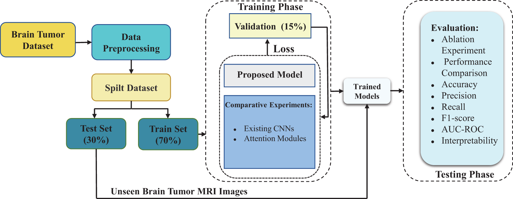
Figure 1: Flowchart of the proposed brain tumor MRI classification technique

3.1 Dataset

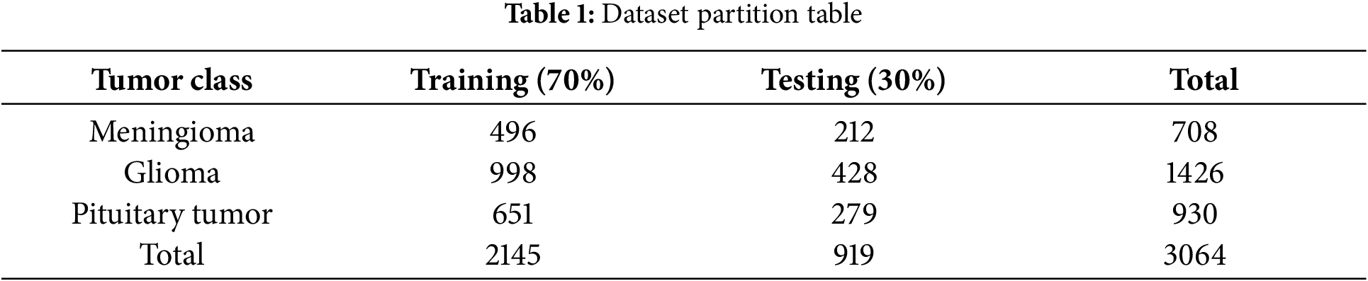
The model presented in our research was trained and tested on a publicly available Figshare dataset which includes MRI scans of three distinct brain tumor types. This dataset [25] comprises a total of 3064 images, including 708 slices of meningioma, 1426 slices of glioma, and 930 slices of pituitary tumor. The original images and tumor masks are stored in.mat format files, which were converted to PNG format images for ease of subsequent experimental analysis. The division of the dataset into training and testing sets is shown in Table 1. During model training, the training set is split into training and validation data to select the optimal parameters.

3.2 Dataset Preprocessing

3.2.1 Segmentation and Size Adjustment

The input for the global branch uses the original whole-brain images, while the input for the local branch uses the tumor region mask files annotated by experts in the dataset. Based on these mask files, we directly segmented the tumor regions. First, we crop the original images according to the range specified in the mask files to extract the complete tumor regions. Subsequently, we fill the non-foreground areas with zeros in the cropped images to focus exclusively on the tumor regions. By inputting the segmented images into the local branch, we can extract and analyze features within the tumor regions in greater detail. Furthermore, the image size is critical for transfer learning methods, as pre-trained CNN models require inputs of specific dimensions. In this study, we resize both the original and segmented images uniformly to pixels to ensure compatibility with the input requirements of the two pre-trained branches.

3.2.2 Gaussian Blur for Image Denoising

Medical imaging data is often affected by high levels of noise, which can compromise the accuracy of subsequent analysis and interpretation. To address this issue, we apply Gaussian blur to smooth the images, thereby reducing interference from details and noise. This method is based on the application of the Gaussian function, as shown in Eq. (1).

(1)

where denotes the value of the Gaussian kernel at position . In this work, we selected an kernel size for the denoising task. The specific value of the standard deviation is automatically calculated by the processing software using a predefined empirical Eq. (2), based on the kernel dimension of the Gaussian kernel and image characteristics such as resolution and noise levels.

(2)

where represents the kernel dimension. The convolution operation is performed on the image using this kernel, resulting in a blurred output.

3.2.3 Image Contrast Enhancement

Contrast-Limited Adaptive Histogram Equalization (CLAHE) technique was introduced during the data preprocessing step to obtain high-quality and high-contrast data. CLAHE is a method used to enhance the contrast of images by applying histogram equalization in different regions to improve the clarity of image details. During the preprocessing step of the dataset, images were divided into 8 × 8-sized grids, and histogram equalization was applied to the pixels in each grid. By experimenting with different methods, we set the clipping limit to 2.0 to achieve more significant contrast enhancement effects. Fig. 2 shows some samples after preprocessing is completed.

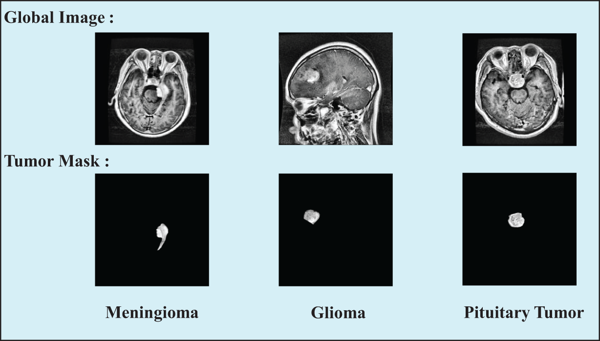
Figure 2: Samples of three types of tumor images in the preprocessed dataset, including the original global images and the segmented tumor region images

3.3 Parallel Dual-Branch for Feature Extraction

The proposed method employs a parallel dual-branch structure, where one branch processes whole-brain images and the other focuses on local tumor images. This design aims to fully capture the features of brain tumor MRI images while minimizing information loss. Based on the characteristics of the input data and the task requirements, we selected appropriate pre-trained network models for each branch. The following section introduces the two branches in detail.

3.3.1 Global Branch: ResNet50 with MHSA

The global branch is designed to capture the overall contextual information of MRI images. In this branch, we utilize the ResNet50 [26] as the backbone network. The core concept of ResNet50 is the introduction of residual connections, where the data flow bypasses certain layers to learn residual functions. This approach allows the network to learn higher-order and more complex feature representations. To improve the model’s capacity for capturing global features, we replaced the final convolutional layer of ResNet50 with MHSA. MHSA effectively captures long-range dependencies and contextual information in images, which is crucial for understanding spatial relationships in complex brain MRI data.

Some studies suggest that MHSA can be applied across the entire network backbone with input resolutions of or [27,28]. However, the resource consumption of the global self-attention mechanism is [29], where denotes the number of input features and represents the dimensionality of each feature. This implies that as the size of the input data increases, both computational and memory requirements grow significantly, particularly when applying the self-attention mechanism across all layers of the network. To address this challenge, some studies propose restricting the use of self-attention mechanisms to the lowest resolution layers of the network [30]. Residual networks consist of multiple stages, with the resolution of feature maps progressively decreasing at each stage. Therefore, we propose replacing the convolutional layer in the final stage of ResNet50 with MHSA. This design effectively captures global information while minimizing computational overhead at high-resolution layers. Given that the MHSA mechanism does not inherently reduce the feature map resolution through down-sampling, we incorporate a average pooling layer with a stride of 2 in place of the convolutional operation at the first replacement layer. This adjustment helps avoid computational bottlenecks when integrating the self-attention mechanism.

In this approach, all attention is focused on a two-dimensional feature map, with relative positional encodings for height and width denoted as and , respectively. The attention mechanism is denoted by , where represents the query encoding, represents the key encoding, and represents the positional encoding, which utilizes relative distance encoding. With the use of multiple heads, the dashed boxes in the diagram (position encoding and value projection) are the only three elements absent in the non-local layer. The schematic diagrams are shown in Fig. 3.

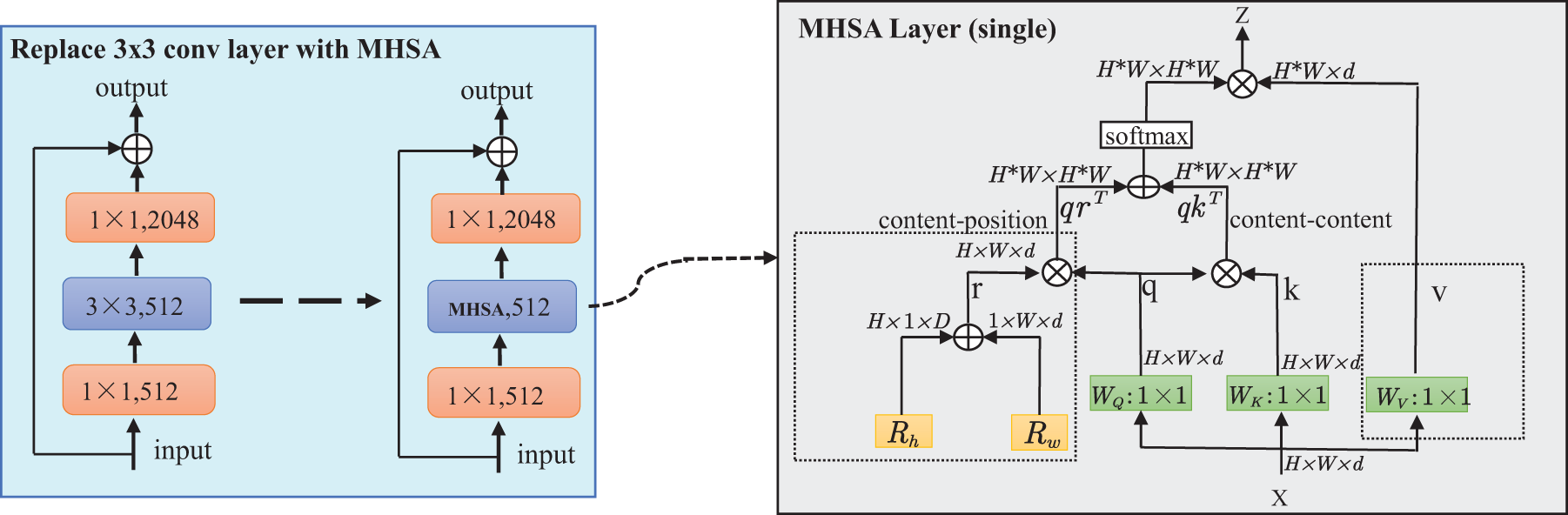
Figure 3: Replacing the 3 × 3 convolutional layers in stage 5 of ResNet50 with MHSA layers and schematic diagram of the MHSA layer

3.3.2 Local Branch: VGG16

VGG16 [31] has been selected as the backbone network for the local branch due to its excellent performance in capturing texture and shape features. VGG16 consists of 13 convolutional layers and 3 fully connected layers, with each convolutional layer employing kernels and a stride of 1. This configuration is designed to preserve spatial resolution while capturing fine-grained local features. The architecture leverages a deep stack of convolutional layers, which sequentially extract hierarchical feature representations, from low-level to high-level information. The outputs of the convolutional layers are typically passed through a ReLU activation function, which effectively mitigates the vanishing gradient problem and accelerates the training process. In addition, VGG16 places a pooling layer after every two convolutional layers, utilizing a max pooling operation with a stride of 2. The pooling layers progressively reduce the spatial dimensions of the feature maps, while retaining critical spatial information. This helps decrease computational complexity and improves the robustness of the extracted features.

This design enhances the efficiency of feature extraction and representation learning in VGG16, making it well-suited for capturing local features, particularly in small tumor regions. The small convolutional kernels and frequent pooling operations are highly effective in processing segmented images of smaller tumor areas, increasing sensitivity to subtle details and thus improving the performance in classification tasks.

3.4 AFFM for Feature Fusion

Local and global features are both indispensable for enhancing the representational capacity of brain tumor classification models. However, simply concatenating or summing these features may not sufficiently highlight the individual importance of local and global characteristics. To address this issue and balance the significance of each branch at different levels, we propose an AFFM to integrate information from both branches. As illustrated in the Fig. 4, we designed AFFM consists of two main components: FSM and IECA. This approach selectively emphasizes the distinct significance of local and global features, thereby optimizing the overall performance of the model.

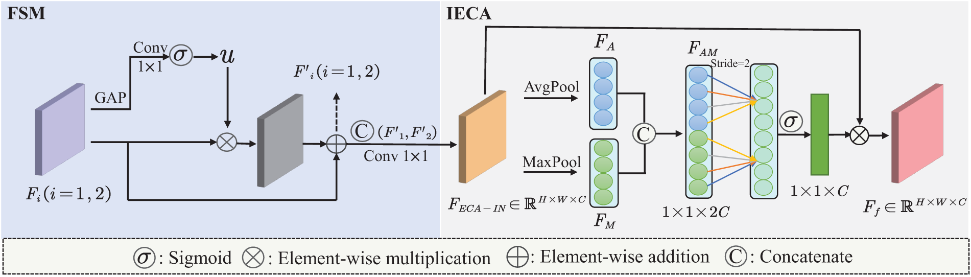
Figure 4: Detailed view of the designed AFFM architecture

3.4.1 FSM

The feature maps representing the outputs from the global and local branches respectively, first undergo global average pooling. These pooled feature maps are then passed through a 1 × 1 convolution layer followed by a sigmoid activation function to evaluate the importance of each feature map within the global context, generating a feature importance vector . The vector represents the importance of each channel in the feature selection module. Next, the original input feature map is multiplied by the feature importance vector , and the resulting product is then added to the original feature map to generate the refined feature map . The processing is illustrated by the following Eq. (3).

(3)

3.4.2 IECA

ECA [32] is a lightweight channel attention mechanism. To meet our task requirements, we applied both max pooling and average pooling to the input of ECA, further enhancing the integration of global and local branch features. Max pooling preserves local salient features, while average pooling aids in extracting global contextual information. The IECA consists of max pooling, average pooling, a 1D convolution layer, and a sigmoid activation function. Additionally, the kernel size of the 1D convolution is adaptively adjusted based on the number of channels and relevant coefficients, thereby optimizing the model’s performance.

As shown in Eq. (4), the feature map fed into the ECA module is obtained by concatenating and , followed by a 1 × 1 convolution.

(4)

where denotes the 1 × 1 convolution and concat represents the concatenation operation.

Assuming , where H and W denote the 1 × 1 height and width of the input feature maps, and C represents the number of channels. The expressions for average pooling, max pooling, and their concatenation are shown in Eq. (5).

(5)

where and are the outputs of global average pooling and global max pooling, respectively, and is the result of their concatenation. represents a set of 2D feature maps.

Then, the global-local dual-branch features, after being fused with attention enhancement, can be represented by as shown in Eq. (6).

(6)

where denotes the sigmoid activation function, and represents the 1D convolution with a kernel size of , which adapts during network training.

3.5 CAB for Addressing Sample Imbalance

Inspired by the CAB mechanism, this approach focuses on identifying more distinctive regional features for each category while ensuring equal treatment across all categories. We introduced this block to assign higher weights to features that are relevant to specific classes while suppressing irrelevant or less important features, thereby improving classification performance for the three brain tumor classes in the presence of sample imbalance.

For the input feature map we first apply a convolution layer to generate a feature map where represents the number of channels required to detect the discriminative regions for each class L. To encourage each of the k feature maps within a class to learn distinct discriminative regions, we randomly drop half of the features during training by setting their values to zero. This results in , which retains only half of the features in each feature map. The importance of each class feature map can be calculated using the Eq. (7). represents the importance scores for each class.

(7)

where represents the -th feature map for the -th class from M″, and GMP denotes global max pooling.

The semantic feature map for the -th class can be represented by Eq. (8).

(8)

where represents the response of the -th feature of the -th class in M′.

By multiplying the importance scores of each class with their corresponding semantic features and then averaging the results, we can obtain the category attention , which highlights the discriminative regions for brain tumor classification, as expressed in Eq. (9).

(9)

Finally, the CAB output is obtained by multiplying input feature map with the attention map element-by-element. As shown in Eq. (10). The schematic diagram is illustrated in Fig. 5.

(10)

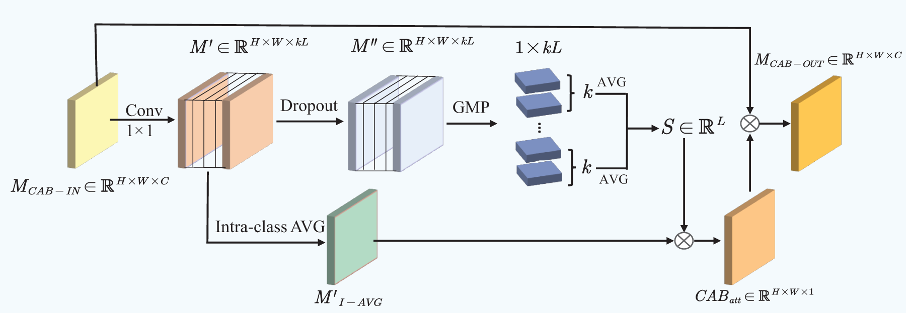
Figure 5: Architectural details of CAB

3.6 Hyperparameter Settings

In this study, we conducted end-to-end training and testing for our model. Given the significant impact of hyperparameter settings on model performance, we performed a series of systematic experiments to optimize training parameters, including batch size, learning rate, optimizer, loss function, and number of training epochs. The selection of hyperparameters was based on preliminary experimental results and recommendations from relevant literature to ensure optimal model performance. During the hyperparameter optimization process, we defined the value ranges for each hyperparameter and systematically evaluated different combinations of hyperparameters using strategies such as grid search or random search to identify the best configuration. We also divided the training dataset into training and validation sets, and the best model configuration was selected based on performance evaluation on the validation set. The final hyperparameter settings are presented in Table 2. For the loss function, we employed the Multi-Class Binary Cross-Entropy Loss. This function is suitable for three-class classification tasks, where each class is treated as an independent binary classification problem [33]. The formula for the loss function is provided in Eq. (11).

(11)

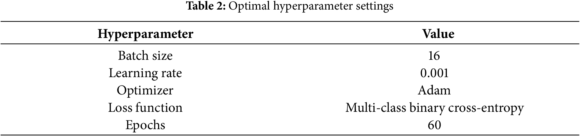
where N is the number of samples, and C is the number of classes. represents the true label of -th instance for -th class, indicating whether the instance belongs to class . is the predicted probability for the -th instance to belong to the -th class.

3.7 Performance Metrics

Evaluating performance metrics is essential in classification research, as different models may prioritize various metrics. In this study, we assessed brain tumor classification using widely accepted metrics: accuracy, precision, recall, and F1-score. All metrics were were calculated based on the confusion matrix, consisting of true positives (TP), true negatives (TN), false positives (FP), and false negatives (FN).

Accuracy serves as a pivotal metric in assessing the correctness of classification models. As shown in the following Eq. (12), accuracy is the ratio of correctly predicted samples to total samples.

(12)

Precision and recall are common parameters used for evaluating classifier performance. In three-class classification task, precision refers to the proportion of samples predicted by the classifier to be a certain class that are actually of that class; recall refers to the proportion of samples actually belonging to a certain class that are correctly predicted by the classifier. The equations are referred to as Eq. (13).

(13)

The F1-score considers both Precision and Recall, providing a comprehensive measure of the classification model’s performance. The expression is seen in Eq. (14).

(14)

Fig. 6 presents the framework of the proposed brain tumor classification model outlined in this paper.

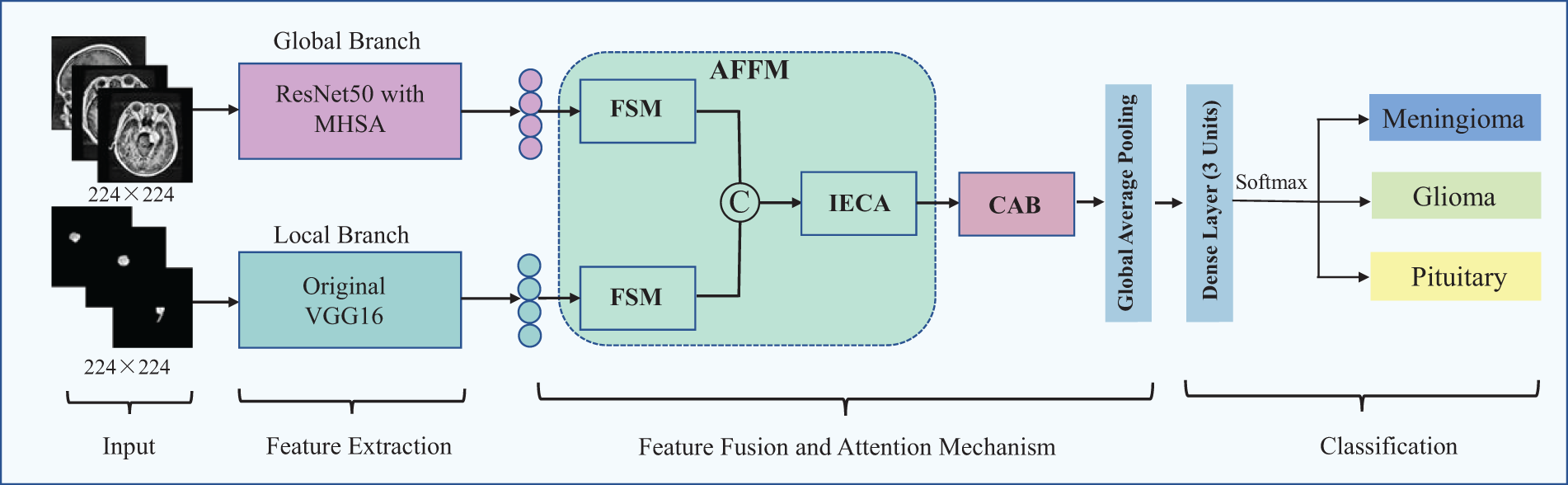
Figure 6: Overall architecture of the proposed brain tumor MRI classification model

4  Experiments Results and Discussion

Experiments were conducted on a computer equipped with an Intel® Core™ i5 processor. The dataset preprocessing was performed using MATLAB R2021a software running on a Windows 10 operating system. The remaining experiments were conducted by connecting to a server via XSHELL software under the Windows 10 operating system and utilizing an NVIDIA GeForce RTX 3090 graphics card for computation. We implemented the proposed model and the CNN models used for comparative analysis using TensorFlow, Keras, and Scikit-Learn frameworks in Python.

4.1 Ablation Experiment

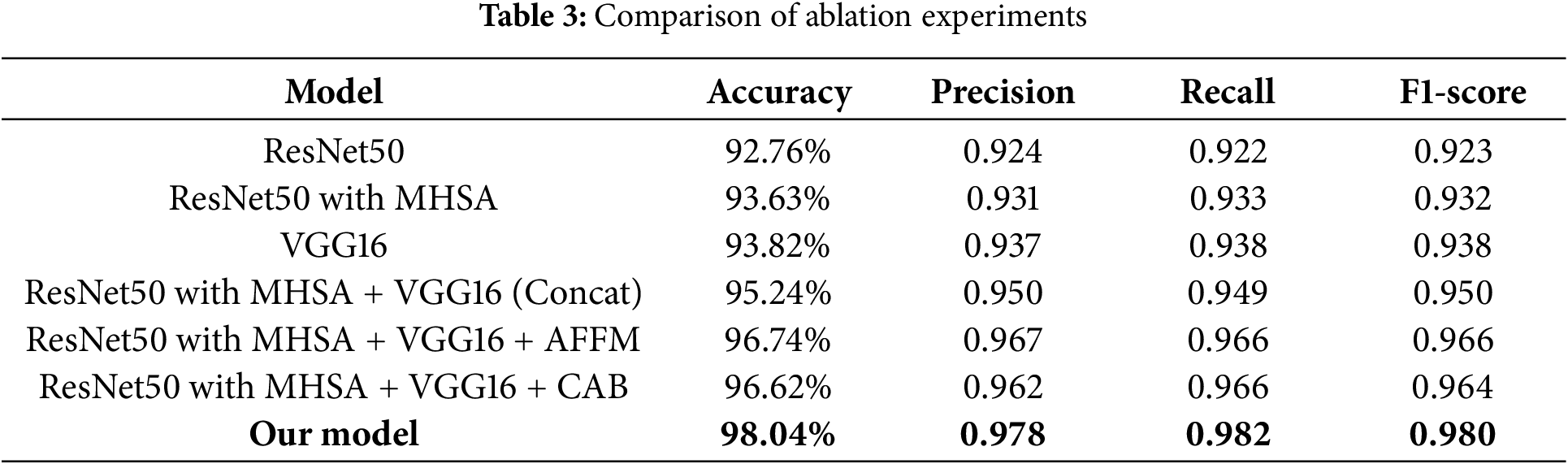
To validate the effectiveness of the our model, we performed a series of ablation experiments, with results summarized in Table 3 (based on 30% testing set). First, to verify the effectiveness of MHSA in enhancing global feature extraction capability, we compared the performance of ResNet50 with and without MHSA. The results showed that adding MHSA improved the accuracy by approximately 1%. Next, we evaluated the performance of the two individual branches by measuring accuracy, precision, recall, and F1-score, establishing baseline performance metrics. Compared to these metrics, our model achieved an accuracy improvement of 3.69% and 3.91%, with other evaluation criteria also showing significant enhancements. Additionally, we evaluated simple feature concatenation without attention mechanisms by comparing its performance to the individual branches. The results showed that concatenation led to performance improvements. Finally, we explored the impact of incorporating the AFFM for enhanced feature fusion and the CAB for addressing sample imbalance within the dual-branch model. The results indicate that while both modules individually contribute to performance gains, their combined application in our model yields superior overall performance.

4.2 Comparative Analysis with Established Models

In this study, we conducted a comparative analysis of the proposed model against classical pre-trained CNN models, including InceptionV3, Xception, GoogleNet, MobileNet, and DenseNet121. To adapt these models for brain tumor classification, we integrated fully connected layers and classification layers, utilizing them in an end-to-end framework.

As shown in Fig. 7, we compared the accuracy and micro-average AUC values of each model on the testing set. The micro-average AUC incorporates results from all classes to reflect overall classification performance. The results indicate that the proposed model achieved the best performance, with an accuracy of 0.980 and an AUC of 0.989, surpassing all other models. The more complex DenseNet121 model also performed well, with an accuracy of 0.943 and an AUC of 0.952. In contrast, Xception showed relatively lower performance, with an accuracy of 0.874 and an AUC of 0.863.

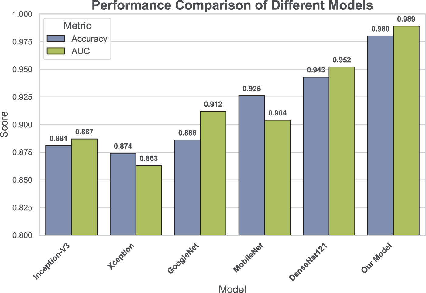
Figure 7: Comparison of accuracy and micro-average AUC across all applied models

As shown in Fig. 8, we generated class-wise heatmaps to compare the precision, recall, and F1-score performance of different models in the classification of gliomas, meningiomas, and pituitary tumors. The heatmap results in Fig. 8a,c indicate that our model outperforms the other models across all performance metrics in the classification of meningiomas and pituitary tumors. This suggests that incorporating CAB substantially improves the model’s ability to classify these two types of brain tumors, even with smaller sample sizes. In the glioma classification heatmap shown in Fig. 8b, proposed model achieves the highest precision and recall, while DenseNet121 also demonstrates high precision and recall. Overall, the heatmap results suggest that the proposed model performs well not only in categories with larger sample sizes but also maintains strong performance in categories with smaller sample sizes.

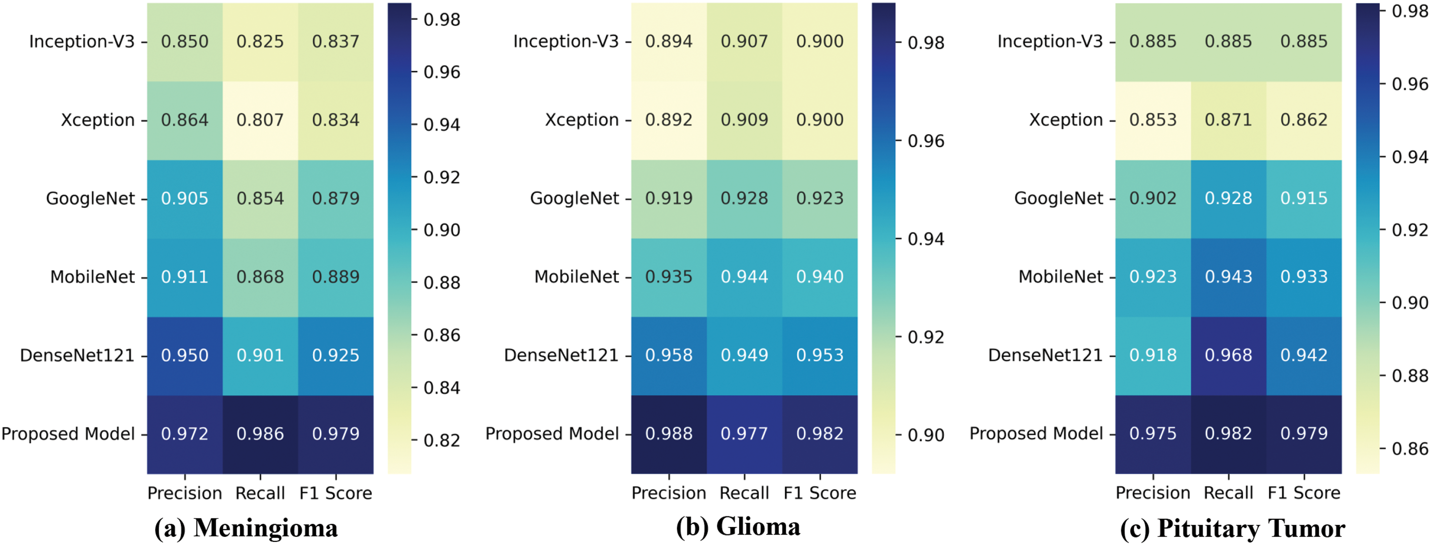
Figure 8: Class-wise heatmaps: (a) Meningioma; (b) Glioma; (c) Pituitary Tumor, depicting precision, recall, and F1-score for each model

Additionally, confusion matrices were generated for each model, as shown in Fig. 9. These matrices visually summarize the classification results for each class, including both correctly and incorrectly classified samples. The results demonstrate that our proposed model has the fewest misclassified samples across all tumor types, confirming its superior accuracy and reliability. Further comparison of the confusion matrix results shows that, without CAB, the baseline CNN model exhibits generally low recognition accuracy for the minority class Meningioma in the imbalanced dataset, with the best-performing model achieving a maximum accuracy of only 90.1%. However, after incorporating CAB, the proposed model’s recognition accuracy for this class increased to 98.6%, representing an improvement of 8.5%. This significant improvement demonstrates the effectiveness of CAB in handling imbalanced datasets, particularly in enhancing the classification accuracy for minority classes.

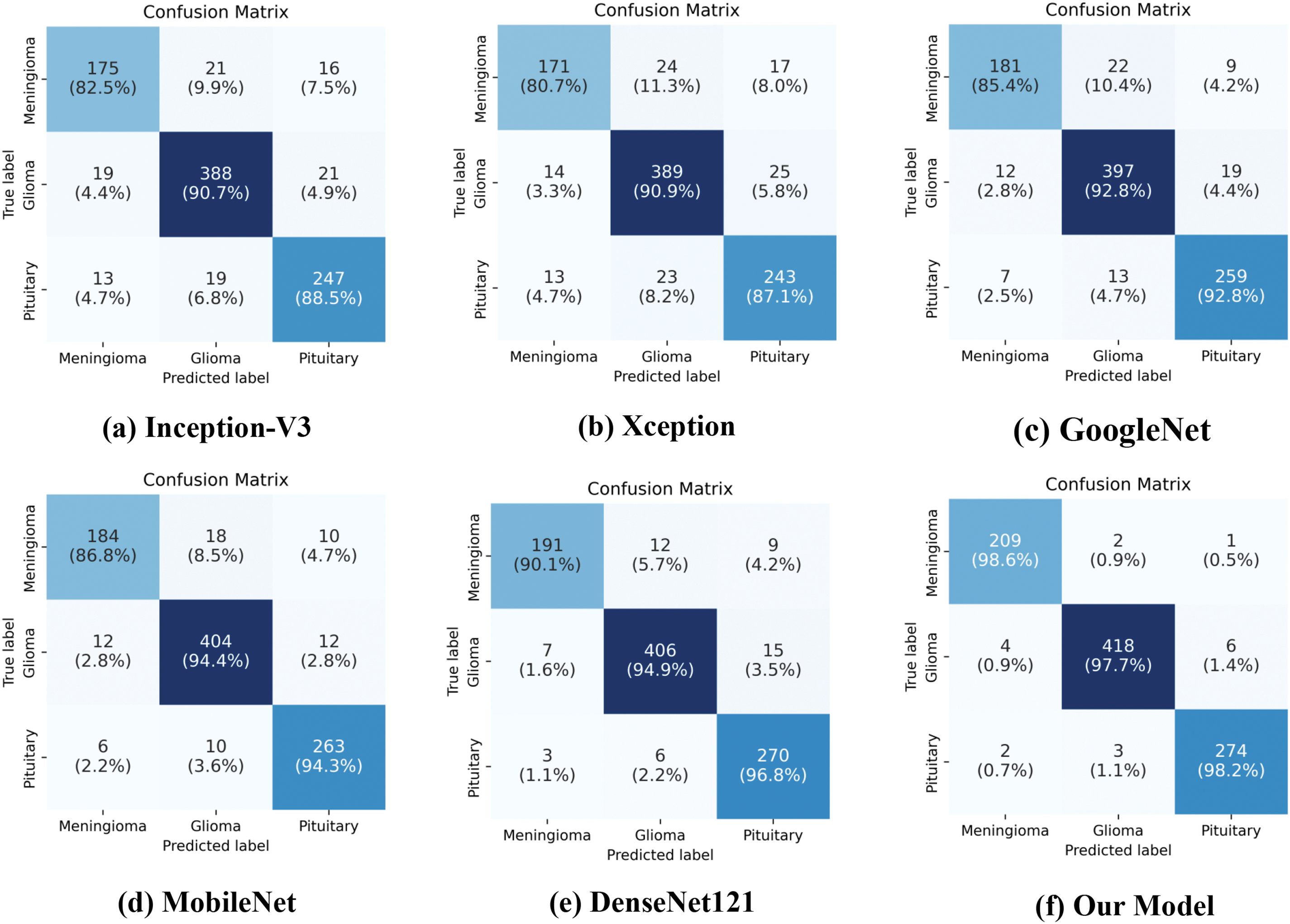
Figure 9: Confusion matrices of various models on the testing set

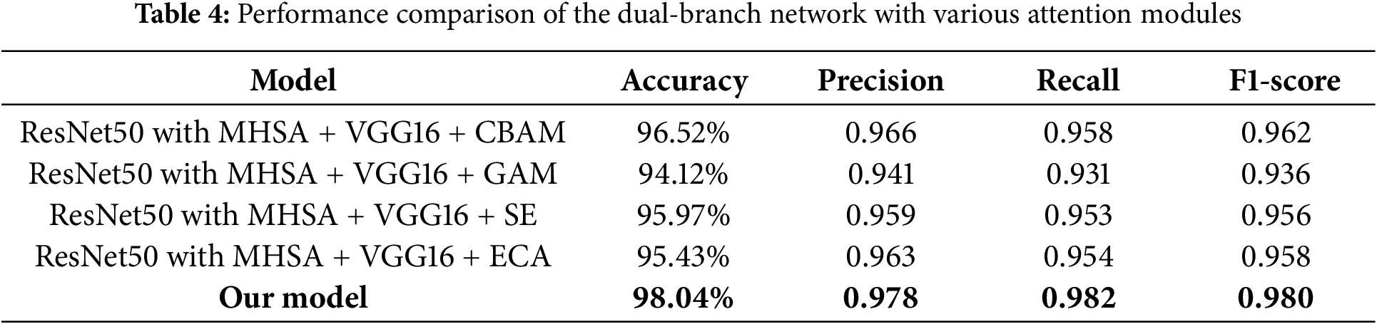
4.3 Performance Comparison of the Dual-Branch Model Combined with Various Attention Modules

To better validate the performance advantages of the proposed attention-enhanced feature fusion dual-branch model, we combined the dual-branch network with several existing attention modules and conducted performance comparison experiments. Specifically, we integrated the dual-branch network with the Convolutional Block Attention Module (CBAM), Global Attention Module (GAM), Squeeze-and-Excitation (SE) module, and ECA module, and systematically evaluated their performance. Through these comparative experiments, we further demonstrated the superiority of the proposed model in feature fusion and attention mechanism application. As shown in Table 4, although the performance of the dual-branch network combined with various attention modules is generally effective, it still outperforms in terms of various performance metrics compared to the model we proposed. Among these combinations, the network integrated with the CBAM module achieved a high accuracy of 96.52%, while the network with the GAM module achieved 94.12%, which is lower than the direct concatenation result. This may be due to the fact that the GAM module suppresses certain key features, making it less suitable for the dual-branch structure we proposed.

4.4 Analysis of the Proposed Model’s Work Effects

To evaluate the learning process of the proposed model, we plotted the accuracy and loss curves for each epoch during the training and testing phases, as shown in Fig. 10. The figure shows that over the course of 60 iterations, the model’s accuracy exhibits an overall upward trend, while the loss gradually decreases. In the early stages of iteration, the model rapidly learns from the data and generalizes well, resulting in a significant increase in accuracy and a sharp reduction in loss. As the number of epochs increases, the accuracy and loss curves gradually stabilize, indicating that the model training is approaching convergence. The choice of 60 epochs was based on performance evaluations from preliminary experiments with varying training durations. These experiments showed that after 60 epochs, the model’s performance stabilized, with no signs of overfitting. Although more epochs might yield slight improvements, the performance gains diminished over time, and the computational cost increased. Therefore, we selected 60 epochs as the final training duration to balance model performance and computational efficiency.

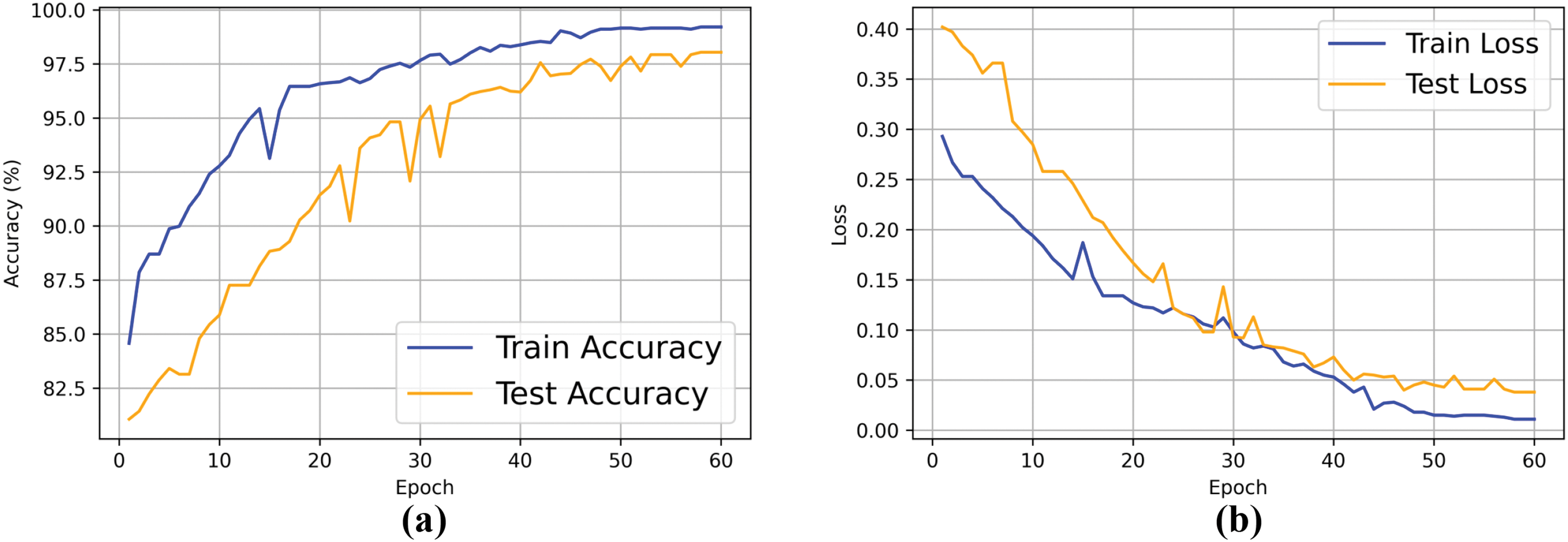
Figure 10: Training and testing accuracy and loss curves of the proposed model. (a) Accuracy curve; (b) Loss curve

The multi-class receiver operating characteristic (ROC) curves for the validation set are shown in Fig. 11a. The model achieved AUC values of 0.988 and 0.984 for the less represented classes of meningioma and pituitary tumors, respectively. For glioma, which had a larger sample size, the AUC reached 0.994. The micro-average AUC was 0.989, further demonstrating the model’s overall effectiveness in handling multi-class classification tasks.

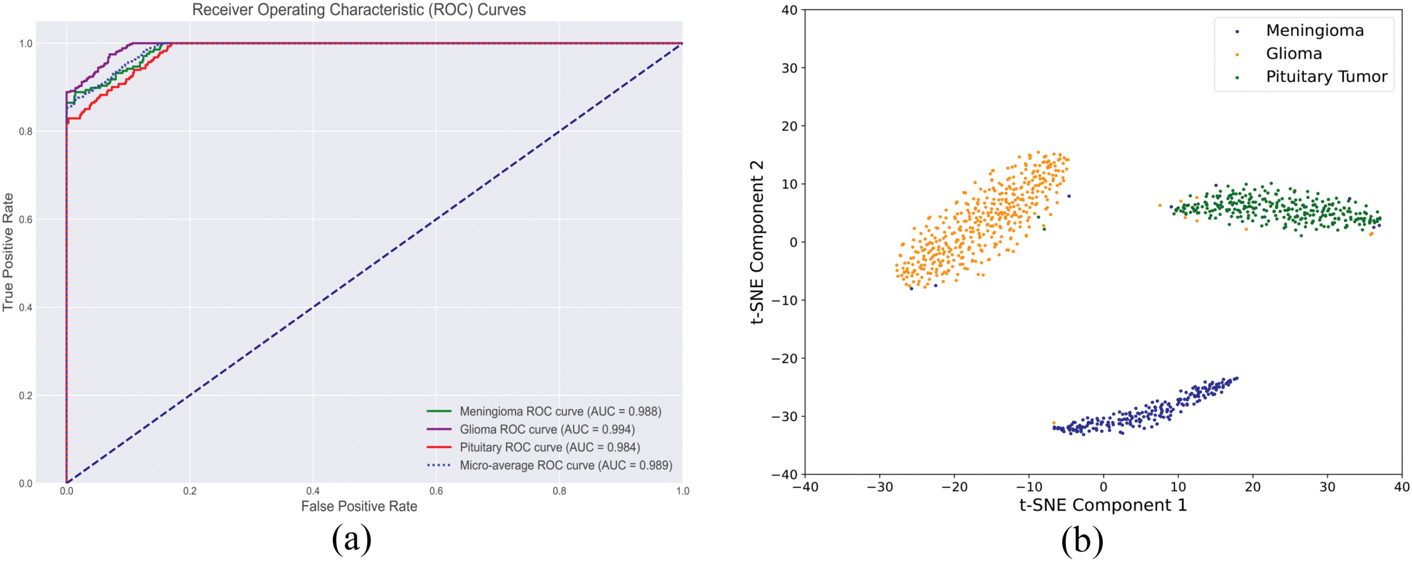
Figure 11: Comprehensive evaluation of the proposed brain tumor classification model: (a) Multi-class ROC curve and (b) Feature space analysis

In addition, to understand the model’s decision-making behavior, we employed t-distributed Stochastic Neighbor Embedding (t-SNE) algorithm to visualize the feature distribution of of testing set samples. The primary objective is to examine whether the feature clusters in the 2D space are closely related to each tumor category. Close intra-class clustering indicates that the model can effectively distinguish between these categories. Fig. 11b demonstrates well-separated and compact clusters, further validating the model’s superior ability to identify and distinguish features associated with different tumor types.

4.5 Feature Interpretability Analysis of the Proposed Dual-Branch Model

To further analyze the interpretability of the model’s decision-making process, this study employed the Local Interpretable Model-agnostic Explanations (LIME) method to identify the key image features that the model relied upon in tumor classification tasks. LIME worked by perturbing individual samples and generating interpretable local models, which effectively visualized the contribution of each feature to the prediction results. As shown in Fig. 12, the model in tumor classification not only focuses on fine-grained features within the tumor region but also takes into account the global contextual information surrounding the tumor. The highlighted yellow areas indicate that the model’s prediction relies on both the local features of the tumor and its spatial relationships with the surrounding environment.

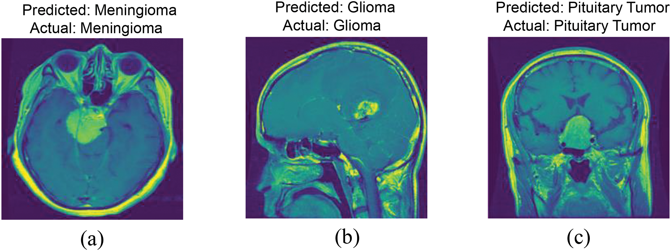
Figure 12: LIME-based feature importance analysis: (a) Meningioma; (b) Glioma; (c) Pituitary Tumor

This indicates that, when making classification decisions, the model did not solely rely on the detailed features within the tumor region, but was capable of integrating local information with global context to make more comprehensive and accurate predictions. This further validated the effectiveness of the proposed dual-branch network design, which enabled the model to simultaneously extract both the microscopic features of the tumor and the macroscopic information of its environment. It highlighted the critical role of local features and global context in tumor classification tasks.

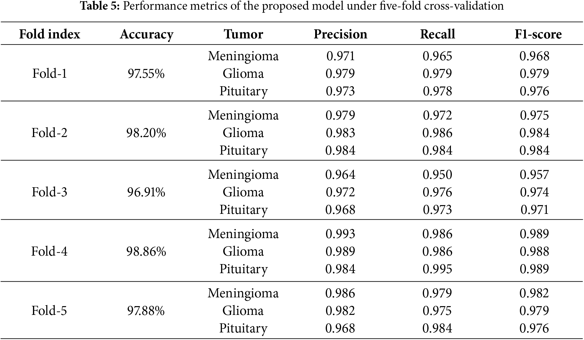
4.6 Five-Fold Cross-Validation

We employed five-fold cross-validation to assess the generalization capability and stability of the proposed model. The entire dataset was proportionally divided into five folds. Each fold contained 141 meningiomas, 285 gliomas, and 186 pituitary tumor samples, totaling 612 samples per fold. In each iteration of cross-validation, four folds were used as the training set, while the remaining fold served as the test set. Through cross-validation, we could more accurately estimate the performance of the proposed method on unknown data, thereby validating the model’s adaptability to different datasets. Table 5 presents the overall accuracy as well as the precision, recall, and F1-scores for each class during the five-fold cross-validation. In the five-fold cross-validation, the proposed method achieved accuracy rates of 97.55%, 98.20%, 96.91%, 98.86%, and 97.88% across the five iterations. These results demonstrate consistent performance, with only minor fluctuations, indicating the model’s robustness and reliability in classification tasks.

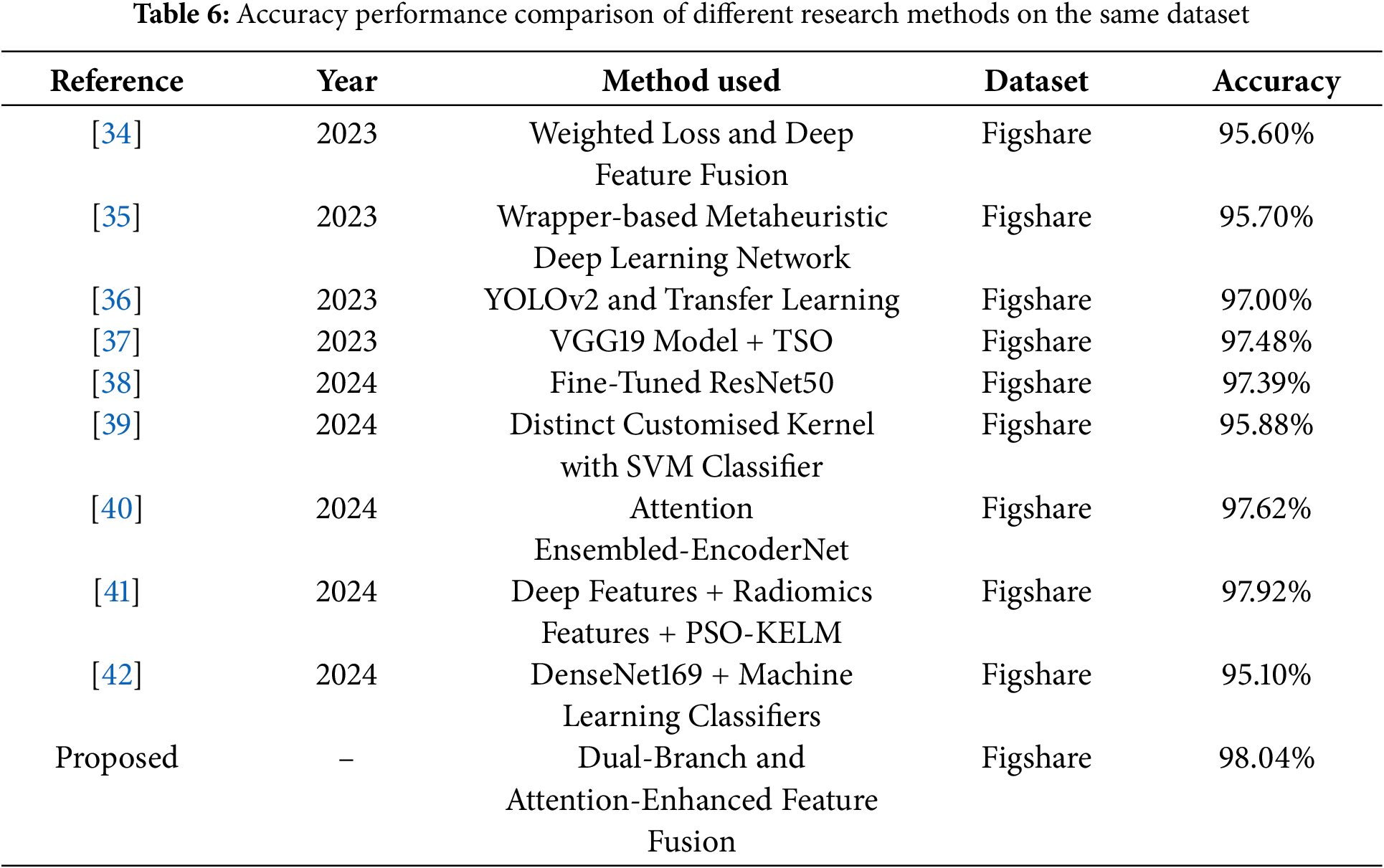
4.7 Comparison of the Proposed Model with State-of-the-Art Study

Several recent studies on the same dataset have been compared with the proposed work in terms of accuracy performance. For example, Deepak et al. [34] proposed a novel class-weighted focal loss and achieves an accuracy of 95.60% using CNN features for classification. Ali et al. [35] proposed wrapper-based metaheuristic deep learning network feature optimization algorithm achieves a brain tumor classification accuracy of 95.70% by selecting the best deep learning network and features. The researchers employed a transfer learning method based on YOLOv2 (you only look once) to classify the extracted tumors, achieving an accuracy of 97% [36]. Poonguzhali et al. [37] employed wiener filtering for preprocessing, utilizes the VGG19 model for feature extraction to optimize performance, and applies the Tunicate Swarm Optimization (TSO) algorithm to fine-tune the hyperparameters of the classification model, achieving a classification accuracy of 97.48% for three types of brain tumors. This research [38] develops a CNN model from scratch, followed by fine-tuning a deep network based on the ResNet50 model, ultimately achieving a classification accuracy of 97.39%. This study [39] proposes a novel framework that integrates four distinct kernel functions into the SVM classifier, achieving an accuracy of 95.88%. This paper [40] proposes an attention-guided CNN architecture that integrates three lightweight encoders at the feature level to combine feature maps with local details, achieving a maximum accuracy of 97.62%. Sandhiya et al. [41] combined deep features extracted from InceptionV3 and DenseNet201, along with radiomics features, and employed a Particle Swarm Optimized Kernel Extreme Learning Machine (PSO-KELM) for classification, achieving an accuracy of 97.92%. Khan et al. [42] extracted features using the DenseNet169 model and fed them into three multi-class machine learning classifiers, achieving a maximum accuracy of 95.10%. Despite the promising results reported in these studies, our proposed method achieved even better accuracy rates, as shown in Table 6.

4.8 Discussion of the Merits and Demerits of the Proposed Model

The key merits of the proposed model lies in its ability to simultaneously capture global context and fine-grained local features, and efficiently fuse them to generate more comprehensive feature representations. The complementary dual-branch structure enables the model to achieve higher classification accuracy and stronger noise robustness when processing complex brain tumor image data, compared to single-branch models. Despite the advantages of the proposed algorithm, there are some demerits. For instance, the dual-branch structure inherently involves higher computational complexity, which may limit its application on devices with limited memory. Especially in resource-constrained environments, the trade-off between model complexity and computational efficiency needs to be carefully considered.

4.9 Limitations of the Study and Future Work

This study has several limitations. First, it utilizes a small publicly available dataset, which may limit the generalizability of the findings. Second, due to the inclusion of tumor segmentation masks in the dataset, the development of a corresponding tumor segmentation model was not pursued. To further validate the effectiveness of our method, we plan to extend the study to larger, multi-center datasets in the future. Additionally, we intend to apply the proposed dual-branch network to the fusion of multimodal information in brain tumor analysis. Considering that not all datasets include tumor mask files, developing an automatic tumor segmentation model is necessary. These extensions will be the focus of future research, thereby enhancing the scientific value and practical application potential of this study.

5  Conclusion

This study proposes a brain tumor MRI classification model based on a global-local dual-branch structure, designed to enhance classification accuracy by addressing the potential omission of small tumor region details during global feature extraction. The model employs a ResNet50 with MHSA branch to capture global contextual information and a VGG16 branch to extract fine-grained local tumor features. Each branch is tailored to its specific task, using whole brain images and segmented tumor region images as inputs, respectively. The effective fusion of features extracted by the two branches is achieved through the designed AFFM. Additionally, the introduction of CAB improves the model’s ability to recognize minority classes, effectively mitigating sample imbalance in the dataset. The ablation and comparative experiments demonstrate that the proposed model outperforms the baseline model and existing CNNs in terms of accuracy and F1-score. The method achieved an accuracy of 98.04%, an F1-score of 0.980, and a micro-average AUC of 0.989 in the classification of three types of brain tumors. The results of five-fold cross-validation further validate the model’s stability and generalization ability, indicating its potential as an effective solution for future brain tumor classification.

Acknowledgement: As I complete this thesis, I would like to express my sincere gratitude for the learning opportunities provided by my school. I am particularly grateful to my advisor, Xinlian Zhou, for her meticulous guidance throughout the process, from topic selection and thesis structure to detailed revisions. I would also like to extend my gratitude to all the editors who took the time to review this paper amidst their busy schedules; your support and suggestions will be immensely beneficial to me.

Funding Statement: The authors received no specific funding for this work.

Author Contributions: The authors confirm their contributions to the paper as follows: conceptualization, methodology, code, and writing: Zhiyong Li; idea guidance, supervision, and English grammar: Xinlian Zhou. All authors reviewed the results and approved the final version of the manuscript.

Availability of Data and Materials: The data that support the findings of this study are openly available in Figshare at http://dx.doi.org/10.6084/m9.figshare.1512427.v5, accessed on 01 January 2025.

Ethics Approval: Not applicable.

Conflicts of Interest: The authors declare no conflicts of interest to report regarding the present study.

References

1. Lapointe S, Perry A, Butowski NA. Primary brain tumours in adults. The Lancet. 2018;392(10145):432–46. [Google Scholar]

2. Pichaivel M, Anbumani G, Theivendren P, Gopal M. An overview of brain tumor. In: Brain tumors. 2022 [cited 2024 Nov 23]. Available from: https://api.semanticscholar.org/CorpusID:246055696. [Google Scholar]

3. Mitusova K, Peltek OO, Karpov TE, Muslimov AR, Zyuzin MV, Timin AS. Overcoming the blood-brain barrier for the therapy of malignant brain tumor: current status and prospects of drug delivery approaches. J Nanobiotechnol. 2022;20(1):412. [Google Scholar]

4. Kristensen B, Priesterbach-Ackley L, Petersen J, Wesseling P. Molecular pathology of tumors of the central nervous system. Ann Oncol. 2019;30(8):1265–78. doi:10.1093/annonc/mdz164. [Google Scholar] [PubMed] [CrossRef]

5. Abd El Kader I, Xu G, Shuai Z, Saminu S, Javaid I, Salim Ahmad I. Differential deep convolutional neural network model for brain tumor classification. Brain Sci. 2021;11(3):352. doi:10.3390/brainsci11030352. [Google Scholar] [PubMed] [CrossRef]

6. Sharif MI, Khan MA, Alhussein M, Aurangzeb K, Raza M. A decision support system for multimodal brain tumor classification using deep learning. Complex Intell Syst. 2021;8:1–14. [Google Scholar]

7. Khan MA, Khan A, Alhaisoni M, Alqahtani A, Alsubai S, Alharbi M, et al. Multimodal brain tumor detection and classification using deep saliency map and improved dragonfly optimization algorithm. Int J Imaging Syst Technol. 2023;33(2):572–87. [Google Scholar]

8. Saba L, Biswas M, Kuppili V, Godia EC, Suri HS, Edla DR, et al. The present and future of deep learning in radiology. Eur J Radiol. 2019;114:14–24. [Google Scholar] [PubMed]

9. Buchlak QD, Esmaili N, Leveque JC, Bennett C, Farrokhi F, Piccardi M. Machine learning applications to neuroimaging for glioma detection and classification: an artificial intelligence augmented systematic review. J Clin Neurosci. 2021;89:177–98. [Google Scholar] [PubMed]

10. Sengupta S, Anastasio MA. A test statistic estimation-based approach for establishing self-interpretable CNN-based binary classifiers. IEEE Trans Med Imaging. 2024;43(5):1753–65. [Google Scholar] [PubMed]

11. Ramakrishna MT, Pothanaicker K, Selvaraj P, Khan SB, Venkatesan VK, Alzahrani S, et al. Leveraging efficientNetB3 in a deep learning framework for high-accuracy MRI tumor classification. Comput Mater Conin. 2024;81(1):867–83. doi:10.32604/cmc.2024.053563. [Google Scholar] [CrossRef]

12. Zhu Z, He X, Qi G, Li Y, Cong B, Liu Y. Brain tumor segmentation based on the fusion of deep semantics and edge information in multimodal MRI. Inf Fusion. 2023;91:376–87. doi:10.1016/j.inffus.2022.10.022. [Google Scholar] [CrossRef]

13. Zhu Z, Sun M, Qi G, Li Y, Gao X, Liu Y. Sparse dynamic volume transUNet with multi-level edge fusion for brain tumor segmentation. Comput Biol Med. 2024;172(8):108284. doi:10.1016/j.compbiomed.2024.108284. [Google Scholar] [PubMed] [CrossRef]

14. Akter A, Nosheen N, Ahmed S, Hossain M, Yousuf MA, Almoyad MAA, et al. Robust clinical applicable CNN and U-Net based algorithm for MRI classification and segmentation for brain tumor. Expert Syst Appl. 2024;238:122347. doi:10.1016/j.eswa.2023.122347. [Google Scholar] [CrossRef]

15. Geetha M, Srinadh V, Janet J, Sumathi S. Hybrid archimedes sine cosine optimization enabled deep learning for multilevel brain tumor classification using mri images. Biomed Signal Process Control. 2024;87:105419. doi:10.1016/j.bspc.2023.105419. [Google Scholar] [CrossRef]

16. Mishra L, Verma S. Graph attention autoencoder inspired CNN based brain tumor classification using MRI. Neurocomputing. 2022;503:236–47. doi:10.1016/j.neucom.2022.06.107. [Google Scholar] [CrossRef]

17. Islam MM, Talukder MA, Uddin MA, Akhter A, Khalid M. Brainnet: precision brain tumor classification with optimized efficientnet architecture. Int J Intell Syst. 2024;2024(1):3583612. doi:10.1155/2024/3583612. [Google Scholar] [CrossRef]

18. Demir F, Akbulut Y, Taşcı B, Demir K. Improving brain tumor classification performance with an effective approach based on new deep learning model named 3ACL from 3D MRI data. Biomed Signal Process Control. 2023;81:104424. doi:10.1016/j.bspc.2022.104424. [Google Scholar] [CrossRef]

19. Ullah MS, Khan MA, Almujally NA, Alhaisoni M, Akram T, Shabaz M. BrainNet: a fusion assisted novel optimal framework of residual blocks and stacked autoencoders for multimodal brain tumor classification. Sci Rep. 2024;14(1):5895. doi:10.1038/s41598-024-56657-3. [Google Scholar] [PubMed] [CrossRef]

20. Arora Y, Gupta S. Brain tumor classification using weighted least square twin support vector machine with fuzzy hyperplane. Eng Appl Artif Intell. 2024;138:109450. doi:10.1016/j.engappai.2024.109450. [Google Scholar] [CrossRef]

21. Alyami J, Rehman A, Almutairi F, Fayyaz AM, Roy S, Saba T, et al. Tumor localization and classification from MRI of brain using deep convolution neural network and Salp swarm algorithm. Cognit Comput. 2024;16(4):2036–46. doi:10.1007/s12559-022-10096-2. [Google Scholar] [CrossRef]

22. Gürsoy E, Kaya Y. Brain-GCN-Net: graph-convolutional neural network for brain tumor identification. Comput Biol Med. 2024;180:108971. doi:10.1016/j.compbiomed.2024.108971. [Google Scholar] [PubMed] [CrossRef]

23. Ravinder M, Saluja G, Allabun S, Alqahtani MS, Abbas M, Othman M, et al. Enhanced brain tumor classification using graph convolutional neural network architecture. Sci Rep. 2023;13(1):14938. [Google Scholar] [PubMed]

24. Pacal I. A novel Swin transformer approach utilizing residual multi-layer perceptron for diagnosing brain tumors in MRI images. Int J Mach Learn Cybern. 2024;15:1–19. [Google Scholar]

25. Cheng J. Brain tumor dataset [Online]. Figshare; 2017 [cited 2024 Nov 23]. Available: http://dx.doi.org/10.6084/m9.figshare.1512427.v5. [Google Scholar]

26. He K, Zhang X, Ren S, Sun J. Deep residual learning for image recognition. In: Proceedings of the IEEE Conference on Computer Vision and Pattern Recognition; 2016; Las Vegas, NV, USA. p. 770–8. [Google Scholar]

27. Zhao H, Jia J, Koltun V. Exploring self-attention for image recognition. In: Proceedings of the IEEE/CVF Conference on Computer Vision and Pattern Recognition; 2020; Seattle, WA, USA. p. 10076–85. [Google Scholar]

28. Dosovitskiy A, Beyer L, Kolesnikov A, Weissenborn D, Zhai X, Unterthiner T, et al. An image is worth 16x16 words: transformers for image recognition at scale. arXiv:201011929. 2020. [Google Scholar]

29. Vaswani A, Shazeer N, Parmar N, Uszkoreit J, Jones L, Gomez AN, et al. Attention is all you need. Adv Neural Inf Process Syst. 2017;30:6000–10. [Google Scholar]

30. Srinivas A, Lin TY, Parmar N, Shlens J, Abbeel P, Vaswani A. Bottleneck transformers for visual recognition. In: Proceedings of the IEEE/CVF Conference on Computer Vision and Pattern Recognition; Nashville, TN, USA; 2021. p. 16519–29. [Google Scholar]

31. Simonyan K, Zisserman A. Very deep convolutional networks for large-scale image recognition. arXiv:14091556. 2014. [Google Scholar]

32. Wang Q, Wu B, Zhu P, Li P, Zuo W, Hu Q. ECA-Net: efficient channel attention for deep convolutional neural networks. In: Proceedings of the IEEE/CVF Conference on Computer Vision and Pattern Recognition; 2020; Seattle, WA, USA. p. 11534–42. [Google Scholar]

33. Mao A, Mohri M, Zhong Y. Cross-entropy loss functions: theoretical analysis and applications. 2023. doi:10.48550/arXiv.2304.07288. [Google Scholar] [CrossRef]

34. Deepak S, Ameer P. Brain tumor categorization from imbalanced MRI dataset using weighted loss and deep feature fusion. Neurocomputing. 2023;520:94–102. doi:10.1016/j.neucom.2022.11.039. [Google Scholar] [CrossRef]

35. Ali MU, Hussain SJ, Zafar A, Bhutta MR, Lee SW. WBM-DLNets: wrapper-based metaheuristic deep learning networks feature optimization for enhancing brain tumor detection. Bioengineering. 2023;10(4):475. doi:10.3390/bioengineering10040475. [Google Scholar] [PubMed] [CrossRef]

36. Sahoo AK, Parida P, Muralibabu K, Dash S. Efficient simultaneous segmentation and classification of brain tumors from MRI scans using deep learning. Biocybern Biomed Eng. 2023;43(3):616–33. doi:10.1016/j.bbe.2023.08.003. [Google Scholar] [CrossRef]

37. Poonguzhali R, Ahmad S, Sivasankar PT, Babu SA, Joshi P, Joshi GP, et al. Automated brain tumor diagnosis using deep residual u-net segmentation model. Comput Mater Contin. 2023;74(1):2179–94. doi:10.32604/cmc.2023.032816. [Google Scholar] [CrossRef]

38. Montoya SFÁ, Rojas AE, Vásquez LFN. Classification of brain tumors: a comparative approach of shallow and deep neural networks. SN Comput Sci. 2024;5(1):142 [Google Scholar]

39. Dheepak G, Anita Christaline J, Vaishali D. MEHW-SVM multi-kernel approach for improved brain tumour classification. IET Image Process. 2024;18(4):856–74. [Google Scholar]

40. Öksüz C, Urhan O, Güllü MK. An integrated convolutional neural network with attention guidance for improved performance of medical image classification. Neural Comput Appl. 2024;36(4):2067–99. [Google Scholar]

41. Sandhiya B, Raja SKS. Deep learning and optimized learning machine for brain tumor classification. Biomed Signal Process Control. 2024;89:105778. [Google Scholar]

42. Khan SUR, Zhao M, Asif S, Chen X. Hybrid-NET: a fusion of DenseNet169 and advanced machine learning classifiers for enhanced brain tumor diagnosis. Int J Imaging Syst Technol. 2024;34(1):e22975. [Google Scholar]