Improved Bidirectional JPS Algorithm for Mobile Robot Path Planning in Complex Environments

1  Introduction

Due to the swift advancement of automation technology and artificial intelligence, the application of mobile robots is growing across various sectors, including industry, service, and healthcare. Path planning for mobile robots is a key area in robotics technology and is the core technology that enables robots to have autonomous navigation capabilities in complex environments [1]. Mobile robot path planning can be categorized into two types: global and local path planning; global path planning calculates an optimal path for the robot from the starting point to the target point under the condition that the environment map is known, while local path planning is to dynamically adjust the path according to the real-time sensing information in the process of the robot moving to avoid the obstacles and other potential hazards on the path [2]. Common global path-planning algorithms consist of traditional methods and intelligent bionic-based approaches. Traditional algorithms typically include the heuristic search-based A* [3] algorithm, the Dijkstra [4] algorithm, the JPS algorithm, and the random sampling-based RRT algorithm [5]; Intelligent algorithms commonly used include particle swarm (PSO) [6] algorithm, ant colony (ACO) [7] algorithm, Grey Wolf (GWO) algorithm [8]. The A* algorithm expands too many useless nodes during the search, which leads to a large amount of computation and long pathfinding time. For this defect, Harbor et al. proposed an optimization algorithm for grid map path planning-JPS algorithm [9]. The algorithm retains the A* heuristic search based on the screening of valuable nodes-called jump points-to eliminate those meaningless redundant nodes, thus reducing the algorithm computation so that the search efficiency has been greatly improved.

Although the JPS algorithm has a large improvement in search speed relative to the A* algorithm, there are also many problems, such as only applicable to the grid environment, the generated paths not being smooth enough, and there may be problems not being able to identify the jumping points efficiently in the complex scene. Scholars at home and abroad have also carried out much research on some problems of the current JPS algorithm. Aiming at the problems of large memory resource consumption, low smoothness of planning paths, and paths too close to obstacles that exist in large-scale complex scenarios of JPS algorithms, Cai et al. [10] and others proposed an improved JPS algorithm, which integrates the security potential field hierarchy function with the improved Floyd algorithm, and finally demonstrated experimentally that this method effectively reduces the consumption of memory resources, improves the smoothness of the paths degree, and ensures the security of the path. Aiming at problems such as more path inflexion points, more intermediate search jump points, more expansion nodes and longer search time in the process of searching for jump points, Liu et al. [11] and others proposed an improved algorithm that dynamically defines the heuristic function and uses dynamic constraint ellipsoids to limit the expansion area, and the improved algorithm has a good performance. For the path-finding algorithms in unstructured and complex scenes, there are problems of long computation time and insufficient optimization of paths; Wei et al. [12] and others proposed to improve the heuristic function based on the jump-point search algorithm by increasing the weights, which effectively minimizes computation time while ensuring that the global path remains the shortest. In addition, by using the differential flatness method to curve-fit the generated path points, the planned global path is made smoother, and this combination not only improves the optimization effect of the path but also enhances the feasibility and practicality of the path. Hou et al. [13] and others proposed a method that combines the artificial potential field method with the hopping point search method, which effectively reduces the number of useless hopping points generated during the expansion process, thus reducing the computation to a certain extent. Additionally, a cubic uniform B-spline curve is utilized for global path smoothing, greatly enhancing the efficiency of path planning.

In recent years, although many excellent researchers have proposed a variety of improvement methods for the problems of the JPS algorithm and achieved significant results, the fast generation of smooth and safe shortest paths in complex scenes is still a topic worthy of in-depth research. In this paper, based on the previous research, an improved Bi-directional JPS algorithm is proposed, which not only ensures the speed of optimal path planning but also ensures the smoothness and safety of the path.

2  Introduction to JPS Algorithm

2.1 JPS Algorithm

The JPS algorithm is an efficient path-planning algorithm that improves the traditional A* algorithm by skipping some unnecessary nodes during the search process, thus reducing the search time of the globally optimal path, and it is known as the JPS algorithm [14].

Before understanding the JPS algorithm, we need to understand the following concepts:

Inferior nodes: We call these inferior nodes if other nodes are directly reachable through x’s parent nodes and the path generation value is less than or equal to the value of reaching through x. These nodes are not explored during the search process. As shown in Fig. 1a, the grey nodes are inferior nodes, and all the nodes, except node 5, have a generation value that is less than the value of arriving through node x from parent node 4, e.g., node 2 has a generation value that is less than the value of arriving through node x from parent node 4, and hence will not be searched, and the rest of the nodes follow this principle. In contrast, in Fig. 1b, for diagonal search, the criterion is changed to abandon the expansion only if the cumulative generation value is less than.

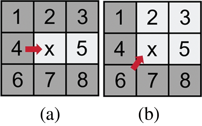
Figure 1: Forward-looking criteria

Natural nodes: If other nodes get minimum path generation cost through x nodes, then they are natural nodes; as in Fig. 1, white nodes except grey inferior nodes are natural nodes, and the search result will add these nodes to Openlist.

Forced neighbours: Node n is said to be a forced neighbour of node x if there are obstacles in the eight neighbours of node x and the distance cost of node x’s parent node p to reach node n is always less than the distance cost of any path that does not pass through node x to reach node n, i.e., node n is a mandatory node for the shortest path. The forced neighbour definition can be summarized into the following two cases; in the first case, parent-child nodes are straight-line relationships as shown in Fig. 2a, where 4 is the parent node, x is the child node, the black node is the obstacle, the shortest path from the parent node 4 to the node 8 is 4 to x and then to 8. Since the shortest path passes through x, the red node 8 is the forced neighbour of the node x. The second parent-child node is a diagonal relationship shown in Fig. 2b, where 6 is the parent node, and x is the child node, the shortest path from parent node 6 to node 8 is 6 to x, and then to 8, similarly red node 8 is a forced neighbour of node x.

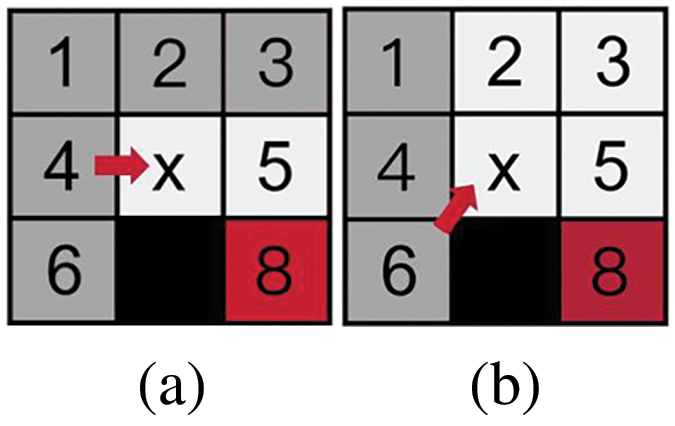
Figure 2: Forced neighbours

The JPS algorithm determines whether the current node is a jump point or not during the search based on the following conditions:

Condition 1: x is a jump point if point x is either a start or an end point;

Condition 2: Point x is a jump point if node x has at least one forced neighbour;

Condition 3: x is a jump point if the parent node p of node x is in the diagonal direction, and there are nodes in the linear direction (horizontal or vertical) of node x that satisfy condition 1 or 2 [15].

The JPS algorithm searches for a jump point that will preferentially move continuously along a straight line direction (e.g., up, down, left, right) until it encounters an obstacle or boundary, at which point the algorithm will record the point of the jump. When jumping in the diagonal direction, the algorithm will check the two neighbouring directions of the diagonal (e.g., up-left and up-right), and if there is an obstacle in one of the directions, the jumping will stop.

Although the jump-point search algorithm has a great improvement in search efficiency compared to the A* algorithm, it also has certain defects because the forced neighbour search strategy leads to the planned path that will definitely be close to the obstacles, so the robot may collide with the obstacles in its travel. As shown in Fig. 3, the path planned by the green circle position algorithm is close to the obstacles, which may cause the robot to collide with the obstacles in the actual movement.

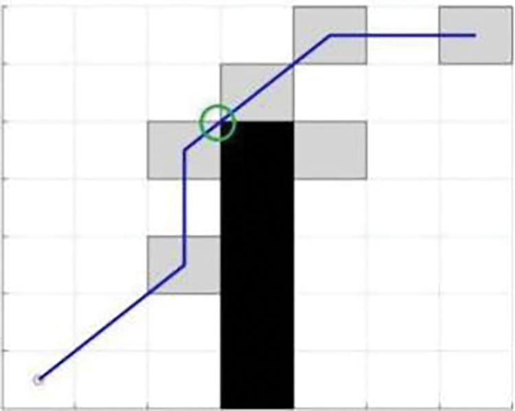
Figure 3: Hazardous locations of the planned path

2.2 Bidirectional JPS Algorithm

The bidirectional JPS algorithm merges the concepts of bidirectional search with the jump optimization strategy inherent in the JPS algorithm. When the algorithm initiates the search, it simultaneously expands to identify jump points from both the starting point and the target point. The pathfinding process concludes when the jump points from both directions overlap, allowing for an efficient path to be determined. As shown in Fig. 4, the red circle indicates the starting point, the green pentagram indicates the target point, and the grey square indicates the searched jump point; the black squares represent obstacles. After the algorithm is run, the search is carried out in mutual directions from the red circle and the green pentagram position, respectively, and the two direction search paths overlap at point A. The pathfinding concludes when the jump points overlap, resulting in the final path, represented as the blue path, which connects the red starting point to the endpoint marked by the green pentagram.

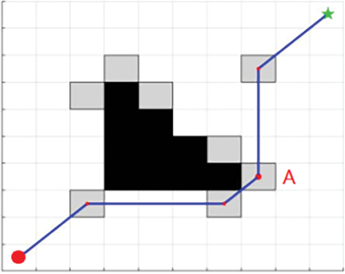
Figure 4: Bidirectional JPS algorithm

Compared with the unidirectional JPS algorithm, the number of search nodes and search time are significantly reduced, but there may be an increase in the number of inflexion points in a wide range of complex scenarios.

3  Improved Bidirectional JPS Algorithm

3.1 Improvement of the Heuristic Function

The traditional JPS algorithm is improved on the basis of the A* algorithm, which is also a heuristic search algorithm, so the evaluation function f(n) of the JPS algorithm is the same as that of the A* algorithm, it also comprises the actual cost function g(n) and the estimated cost function h(n), in which n denotes the current node, and the smaller the value of the f(n) substitution denotes the shorter the path to be planned [16].

(1)

h(n) is the heuristic function of the JPS algorithm, which plays the role of direction guide for planning the global path, and the specific generation value is usually calculated in the following ways:

1. Manhattan Distance:

(2)

2. Euclidean Distance:

(3)

3. Chebyshev Distance:

(4)

Manhattan distance is applicable to the scenario that can only move in horizontal and vertical directions, while Euclidean distance is applicable to the case that can move in any direction, and Chebyshev distance is applicable to the case that can move in eight directions (including diagonal). In this paper, the Euclidean distance formula is used for cost calculation, and the algorithm search speed and direction accuracy are optimised by dynamically defining the weight factor and the specific improvement formula of the heuristic function is shown in Eq. (5).

(5)

where h*(n) is the improved heuristic function, w is the dynamic weight factor of the improved heuristic function, r represents the Euclidean distance between the current node and the target point, d is the Euclidean distance from the starting point to the target point, (xm, ym), (xn, yn) denotes the start point and the target point, respectively, with the continuous expansion of the search area, the current node gets closer to the target point, the value of w becomes smaller, the more the weight factor, at this time in order to find the optimal path, the focus is to find the optimal path.

3.2 Redundant Node Optimisation

The original JPS algorithm searches for a large number of useless jumps when finding a path and stores them, which leads to a large amount of computation and redundant nodes, long path distances and other problems. To address these problems, this paper proposes a pruning strategy for path optimisation, which eliminates redundant nodes and optimises the shortest path. The basic principle of the pruning strategy is shown in Fig. 5; the small red circle in the figure indicates the starting point, the small red flag indicates the target point, the black path is the original JPS planning path, the red path is the optimised path, we can clearly see that there are three paths that the pruning strategy has optimised. In the first AC segment, the original algorithm path for AB→BC, according to the principle of the triangle, any two sides of the sum must be greater than the third side. We learn that the distance of the AC segment must be less than the distance of AB + BC, so the redundant nodes at point B are eliminated. Similarly, the E point and H point also belong to redundant nodes, DF and GJ distance is also less than the original algorithm planning path distance.

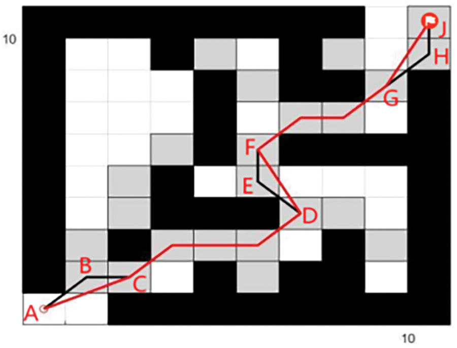
Figure 5: Path optimisation process

The exact steps of optimisation are shown below:

(1) Extract every point of the original path planned by the algorithm, traverse all nodes and perform redundant node removal using the pruning strategy of this paper;

(2) Examine if an obstacle lies between the current node and the node that follows; if there is an obstacle, then the original path is retained; if there is no obstacle, then a new path is generated;

(3) Use this method to cycle through the subsequent nodes to determine whether collision detection occurs, eliminate redundant nodes in the global path, and generate the final path, i.e., the shortest path.

3.3 Introduction of Bezier Curves

French engineer Pierre Bezier derives bezier curves based on Bernstein polynomials. Since he was the first to study this method of vector plotting curves and provided specific formulas for them, they are called Bezier curves because they are named after his last name. Bezier curves are now widely used in robotics because of their simple structure, smoothness and constant endpoints, and are often used to smooth path turning points and optimise robot trajectories. The principle is to use a set of control points to define the shape of the curve, and the location and number of these control points govern the characteristics of the curve. In this paper, we introduce a second-order Bezier curve to smooth the turning points of the planned path in the algorithm, as shown in Fig. 6a, P0 corresponds to the start endpoint, P1 is the turning point, P2 is the target endpoint, a is the left endpoint of the green line segment, and b is the right endpoint of the green line segment. The three points, P0, P1, and P2, are fixed and unchanging, but the green line segment is subject to change with the change of t. We first give a scaling factor, t, and then we use the control points to define the shape of the curve, which determines the characteristics of the curve. We are first given the scale factor t ∈ [0, 1], a = (1–t)P0 + tP1, which is the result of linear interpolation on the P0P1 line segment, and b = (1–t)P1 + tP2, which is the result of linear interpolation on the P1P2 line segment, and the second-order Bezier’s formula is shown in Eq. (6) [17]:

(6)

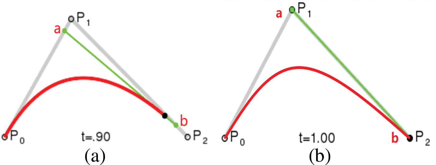
Figure 6: Second-order Bezier curve fitting procedure

When t = 0, P2(t) = P0, so the starting point and P0 coincide, 0 < t < 1, the curve point is the black point in the figure, t = 1, the target point coincides with the P2 point, and finally, the curve formed by the left endpoint P0 the right endpoint P2 is both the fitted second-order Bezier curve. By fitting a second-order Bezier curve to the three points P0, P1 and P2, the red curve shown in Fig. 6b is finally obtained.

3.4 Fusion DWA Algorithm

The DWA algorithm is a real-time dynamic planning method for localised paths of mobile robots, by taking the dynamic characteristics of the robot and the environmental obstacles into account, it creates safe and efficient motion trajectories [18].

The basic steps of the algorithm include: Firstly, defining a dynamic window based on the current velocity and acceleration of the robot, which represents the range of velocities that can be reached in the future period; secondly, sampling multiple possible combinations of velocities (linear and angular velocities) within the dynamic window; immediately afterwards, predicting a motion trajectory for each combination of velocities, and evaluating its safety (distance from obstacles), target proximity (distance from the target) and motion efficiency (smoothness of velocity changes), and score each trajectory according to the evaluation function; Then, based on the scores, the optimal trajectory is selected to be the next motion instruction for the robot, and the robot executes the motion according to the velocity combination selected by the instruction. Aiming at the JPS algorithm generating paths close to the obstacles, which may cause safety hazards, as well as in the specific kinds of movement that may appear unknown obstacles problem, this paper will be the DWA algorithm and bidirectional JPS algorithm fusion to achieve real-time dynamic path planning.

3.4.1 Analysis of Robot Kinematics Models

The establishment of the robot kinematic model is the premise of using the dynamic window method; this paper takes the four-wheel-drive differential robot model shown in Fig. 7 as the object of study, and its motion state can be expressed by the robot’s linear velocity Vt, angular velocity ωt, four wheels are placed at the four corners of the rectangle or square and are parallel to each other. The four wheels are located on the four corners of the rectangle or the square, with the wheels being parallel to each other. VA, VB, VC, and VD are the rotational speeds of the four wheels A, B, C, D, respectively, which are the rotational speeds of the motors; Vx is the translation speed of the vehicle along the X-axis, and ω is the rotational angular speed of the vehicle along the Z-axis; is half the wheelbase D of the trolley, is half the wheelbase H of the trolley. Solving for the state of motion of the trolley, the solution gives the speed of each of the four wheels as shown in Eq. (7):

(7)

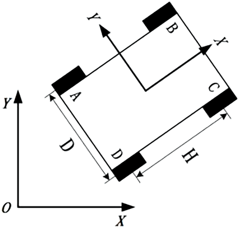
Figure 7: Kinematic modelling of 4WD differential robots

3.4.2 Evaluation Function

Since there will be multiple sets of motion trajectories sampled in velocity space, in order to evaluate multiple sets of motion trajectories and determine the optimal trajectories, these trajectories need to be evaluated and analysed using a set of evaluation criteria [19], the specific evaluation function is shown in Eq. (8):

(8)

When the value of G(v,w) is the smallest, the optimal path is obtained, where τ denotes the smoothing coefficient. Heading(v,ω) is the azimuth evaluation function, which is used to make the robot’s orientation continuously converge to the end direction; the smaller the value means the smaller the azimuth angle with the endpoint; Goal(v,ω), acting as the objective evaluation function, is used to gauge the distance from the end of the robot’s local path to the endpoint, and the distance to the endpoint is continuously shortened by the function; Path(v,ω) is the path evaluation function designed to work out the distance from the endpoint of the trajectory towards the global path; Occ(v,ω) is the obstacle evaluation function that is used to gauge the distance from the robot trajectory to the obstacle if the distance from the robot’s trajectory to the obstacle is greater than the robot’s radius, there is no risk of collision; on the contrary, it means that there is a high risk of collision, and the trajectory is discarded. α, β, γ, σ is the weighting coefficient of each evaluation function [20].

4  Simulation Experiment and Analysis

To verify the efficacy of the I-BJPS algorithm proposed in this paper within complex environments, different algorithms are compared to verify and analyse each improvement point. The simulation uses the following equipment configuration: the operating system is 64-bit Windows 10, the processor is i5-9400H, the discrete graphics card is GTX1060 6G, the main frequency is 2.9 GHz, the memory is 16 GB, and the simulation running platform is MATLAB R2019a.

4.1 Improved Heuristic Function and Redundant Node Optimisation Validation

As shown in Figs. 8–10, three different sizes of 30 × 30, 50 × 50 and 80 × 80 raster maps of complex scenes are used to validate the improved heuristic function and node optimization in simulation experiments respectively, with the small red circle Start on the map indicating the starting point, the green pentagram Target indicating the target point, the black part indicating the obstacles, the white box indicating the idle area, and the grey squares indicating the algorithms searched jump points. All three maps (a) denote the original JPS algorithm (JPS); (b) denote the original Bi-directional JPS algorithm (BJPS); (c) denote the Bi-directional JPS algorithm after improving the heuristic function (IHF-BJPS); (d) denote the Bi-directional JPS algorithm after improving the heuristic function and node optimization (IHFNO-BJPS). Table 1 shows the comparison results of the number of evaluation nodes, number of inflexion points, path length, and running time of different algorithms for the experiments conducted in the raster maps of the designed complex scenarios.

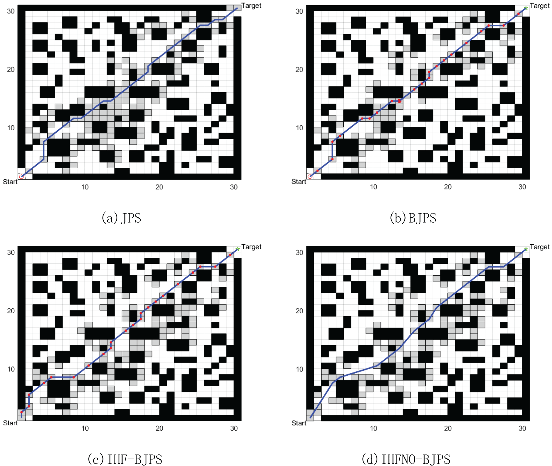
Figure 8: 30 × 30 complex environment raster map path comparison

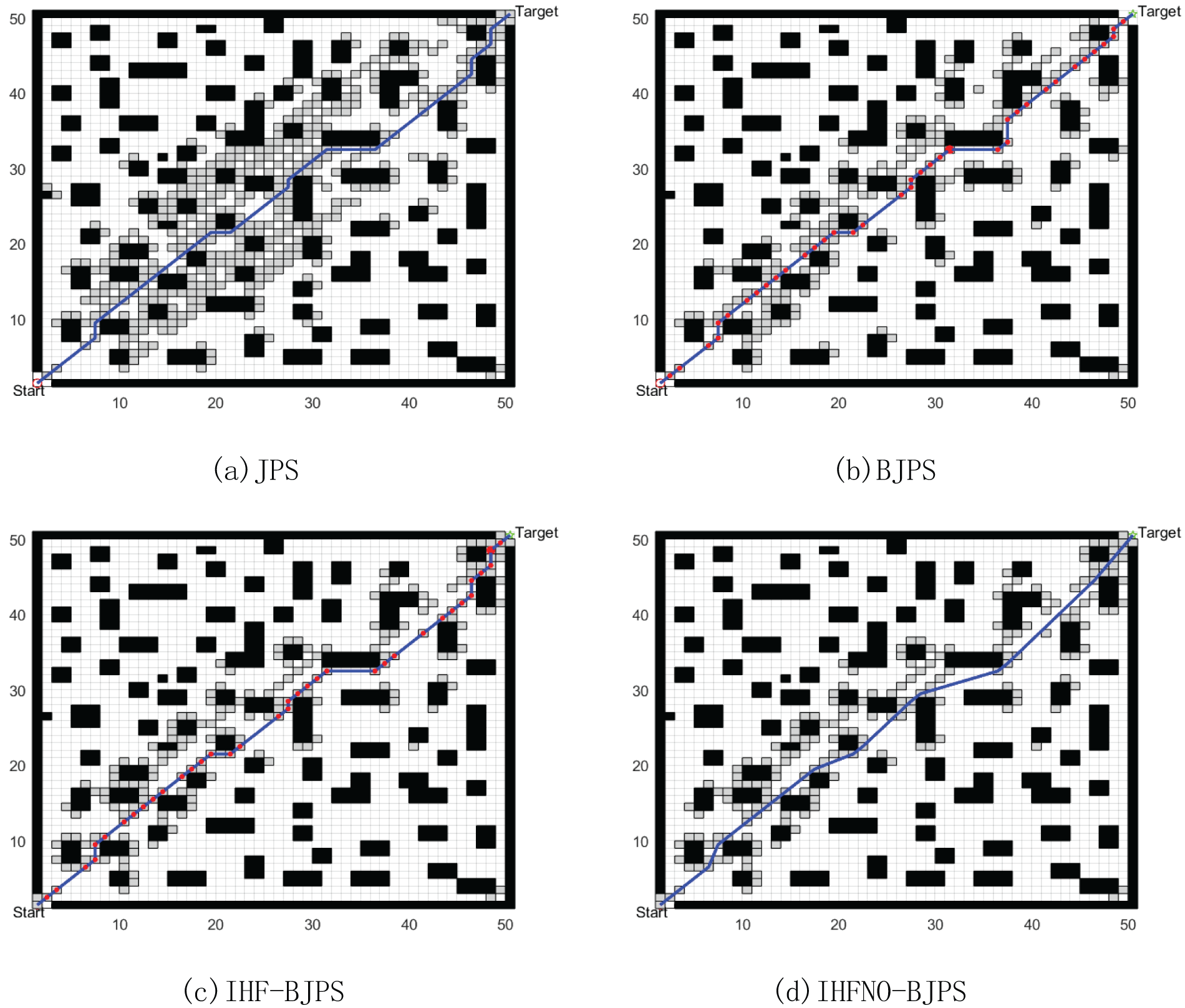
Figure 9: 50 × 50 complex environment raster map path comparison

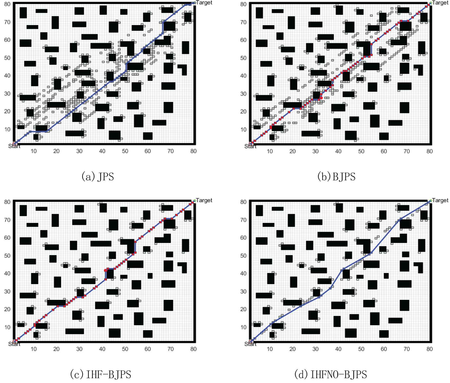
Figure 10: 80 × 80 complex environment raster map path comparison

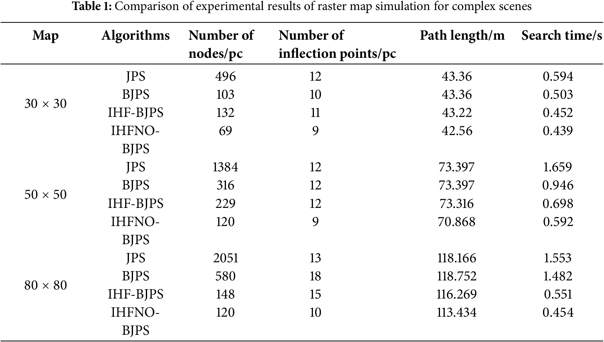
From Figs. 8–10 and Table 1, it can be seen that the original JPS algorithm and the original BJPS algorithm plan the same path length in a 30 × 30 raster map of a complex environment, but the search time increases by 0.091 s and the number of evaluation nodes and the number of inflexion points relatively decreases. Compared to the original BJPS algorithm, the BJPS algorithm with the improved heuristic function has a slight increase in the number of evaluated nodes and the number of inflexion points; however, the length of the path is decreased, and the search speed is remarkably accelerated. The BJPS algorithm combining the improved heuristic function and node optimisation shows some improvement in all aspects.

In a 50 × 50 raster map of a complex environment, the path lengths planned by the original JPS algorithm and the original BJPS algorithm remain the same, but the search time increases significantly, and the number of evaluation nodes and the number of inflexion points remain the same. Upon improving the heuristic function, the BJPS algorithm reduces the number of evaluation nodes and the path length, and the search speed is significantly increased, while the improvement of the BJPS algorithm after improving the heuristic function and the node optimisation is more obvious compared to the 30 × 30 map in terms of the improvement of the indexes.

In an 80 × 80 raster map of a complex environment, the original JPS algorithm and the original BJPS algorithm plan almost the same path length and search time, but the number of evaluation nodes is reduced significantly while the number of path inflexion points is increased. Compared with the original BJPS algorithm, the BJPS algorithm with improved heuristic function reduces the number of evaluation nodes and path length, and the search speed is significantly accelerated. The BJPS algorithm, combining the improved heuristic function and node optimisation, has significantly improved performance in all aspects.

As a result, the improved algorithm is able to plan shorter paths and reduce the number of inflexion points while significantly improving the search efficiency under larger maps and more complex scenes. These results reveal that the proposed refined strategy can effectively heighten the path-planning performance of mobile robots under different complex environments.

4.2 Introducing Bezier Curve Verification

Although the improved I-BJPS algorithm has obvious improvement in path distance and search efficiency, there are turning points in the path, so this paper introduces the second-order Bezier curve to optimise the turning points and smooth the global path. In order to verify the effectiveness of the algorithm after fusing Bezier curves, this paper designs two kinds of raster maps, 30 × 30 and 50 × 50, for experiments, as shown in Fig. 11, with the red small circle Start as the starting point, and the green five-pointed star Target as the goal point. Fig. 11a and c both shows the I-BJPS algorithm before fusing the Bezier curves, and Fig. 11b and d both shows the I-BJPS algorithm after fusing the Bezier curves; the blue paths in Fig. 11a and c denote paths planned by the unfused curves, the red curves in Fig. 11b and d denote paths of the unfused curves, and the black line segments denote the curves after fitting the turning points.

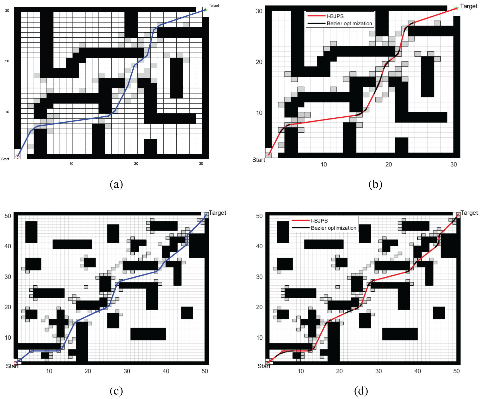
Figure 11: Comparison of different map fusion Bessel curve paths

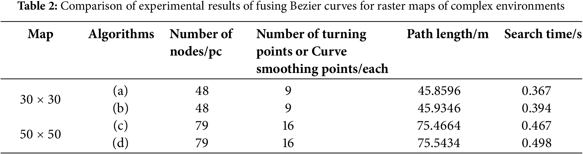
As we can see from Fig. 11 and shown in Table 2, the number of nodes evaluated by the algorithm after fusing the curves did not change, and all the turning points were fitted by the curves, resulting in smoother paths, although the search time increased somewhat compared to the previous one. This suggests that although the smoothness of the path has been improved, it may have led to a decrease in search efficiency in terms of computational complexity. Therefore, in practical applications, the relationship between path smoothness and search time needs to be weighed in order to achieve the best path-planning results.

4.3 Validation of the Fusion DWA Algorithm

To verify the efficacy of the fusion DWA algorithm, this paper uses a 30 × 30 complex environment raster map to conduct real-time dynamic planning simulation experiments. As shown in Fig. 12 for the I-BJPS algorithm fusion DWA algorithm real-time dynamic planning process, the Start point indicates the starting point, the Target point indicates the target point, dynamic planning after the start of the four-wheel drive differential car with a given acceleration from the initial point to the destination point, the maximum speed is set to 1.5 m/s. Fig. 12a for the algorithm to generate a global path, where the red paths are the paths planned before fusing the Bessel curves, and the black curves are the second-order Bessel fitted curves; Fig. 12b for the global path in the planning of the global path to add unknown moving and static obstacles real-time re-planned path, the small yellow squares indicate the real-time re-planning from the starting point to the target point. Unknown dynamic and static obstacles are added to the real-time re-planned path; the yellow squares indicate the dynamic obstacles from point A to point B, and the grey squares on the original path are the static obstacles added temporarily; Fig. 12c is the result of the final dynamic path planning, the blue solid line is the final path of the cart, and the dotted line is the initially planned global path, and it can be clearly seen that the dynamically planned path successfully avoids the global planned path. Known and unknown obstacles in the path, which greatly improves its safety; Fig. 12d shows the real-time changes in linear and angular velocities of the 4WD vehicle when the DWA algorithm is running, and Fig. 12e records the real-time attitude angle changes of the 4WD vehicle, which makes it safer to avoid known and unknown obstacles in the path by constraining its linear, angular velocities and attitude angles.

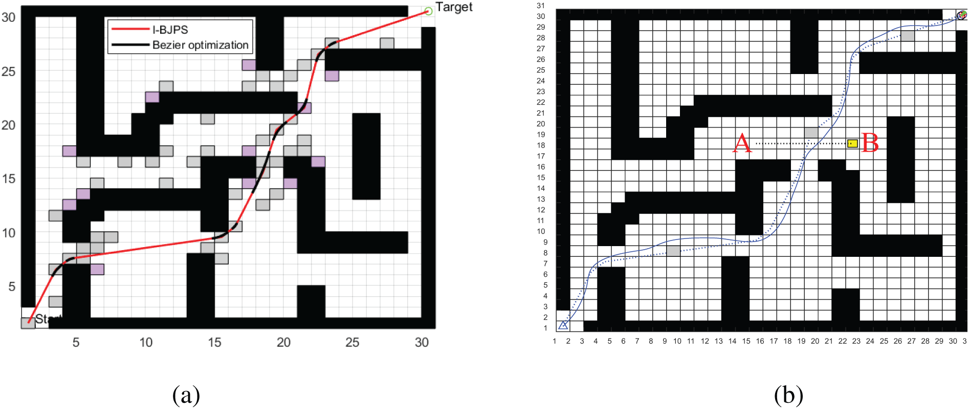
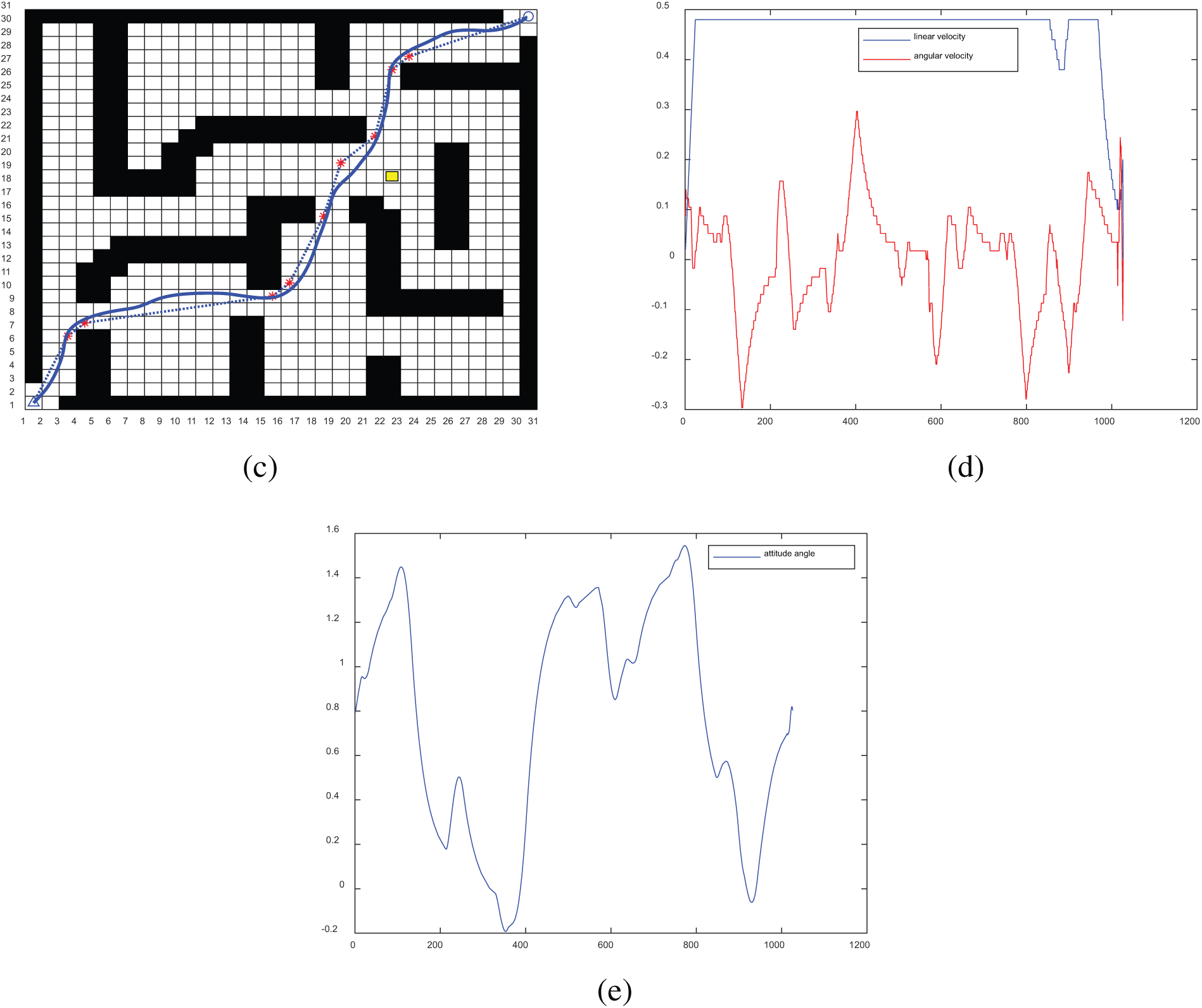
Figure 12: I-BJPS fusion DWA dynamic planning process

4.4 Experimental Comparison of Different Algorithms

In order to verify the effectiveness of the improved bidirectional JPS algorithm in this paper, we designed a raster map in a 30 × 30, 50 × 50 complex environment and cited the improved classical Astar algorithm and our improved bidirectional jumping point algorithm for comparative simulation experiments. In Fig. 13, the Start represents the starting point, the green pentagram Target represents the goal point, the red path denotes the planned global path, and the black box denotes the obstacles. Fig. 13a and c shows the global paths planned by the improved Astar algorithm under different maps, where the grey boxes indicate the nodes traversed by the algorithm during the search. Fig. 13b and d shows the global paths planned by I-BJPS under different maps, respectively, where light grey boxes indicate the jump points of the algorithm.

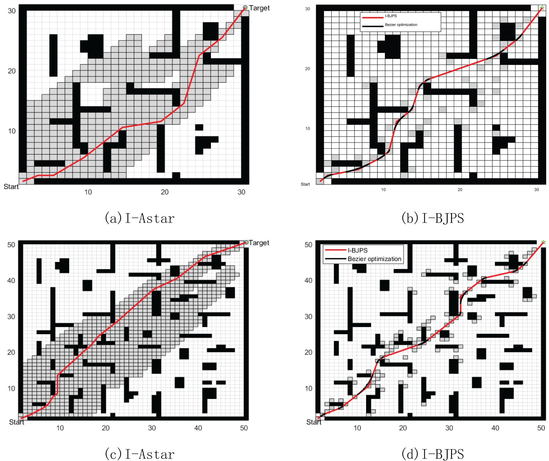
Figure 13: Algorithm comparison experiment

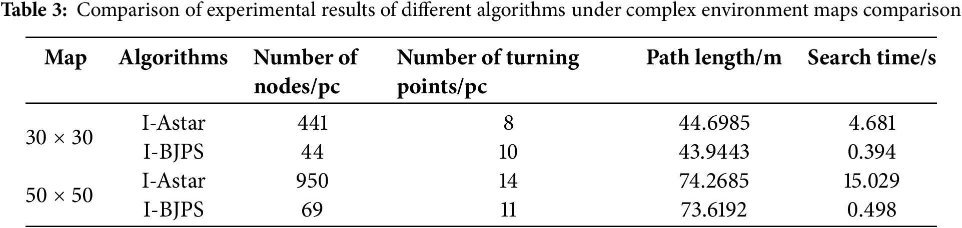
Based on the analysis of the results in Fig. 13 and Table 3, it can be seen that our improved algorithm significantly reduces the number of expanding nodes during the search process, which shortens the search time by at least ten times compared to the classical Astar improved algorithm. However, the optimisation of the path length is not conspicuous as the paths planned by the enhanced A-algorithm are nearly the shortest path. Therefore, in larger and more complex environments, our improved algorithm is able to plan a smooth and safe optimal global path more quickly.

5  Real Machine Experiment and Analysis

5.1 Experimental Platform

In this paper, the improved algorithm is verified using a 4WD differential mobile platform built by ourselves, as shown in Fig. 14, which mainly consists of a 4WD differential chassis, a ROS main control board (NVIDIA Jeston Nano B01), a chassis control board (STM32F407), and a 3D LiDAR (Livox Mid-360). Among them, the 4WD differential chassis is driven by a DC brushless motor, with a distance of 0.206 m between the centres of the wheels on both sides and a maximum speed of 1.2 m/s. Based on the robot operating system (ROS), the tracking and control code is written, and the motion instructions for controlling the robot are generated using Python and C++, and the system communication is established through the serial port and the USB data line with the bottom layer establishes the system communication to achieve the behavioural control of the 4WD differential mobile platform.

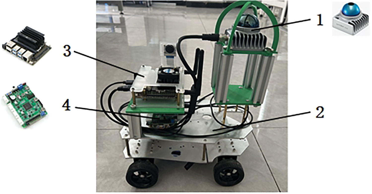
Figure 14: 4WD differential mobile platform 1.3D LIDAR (Livox Mid-360) 2.4WD differential chassis 3.NVIDIA Jeston Nano B01 4.STM32F407 microcontroller

5.2 Experiments and Analyses

The selected experimental scene in this paper is the indoor complex scene shown in Fig. 15, in which the position of the mobile platform is the starting point, the red circle position is the target point, the blue boxes on both sides are the boundaries, and the cardboard box and the black plastic box in the middle are the obstacles.

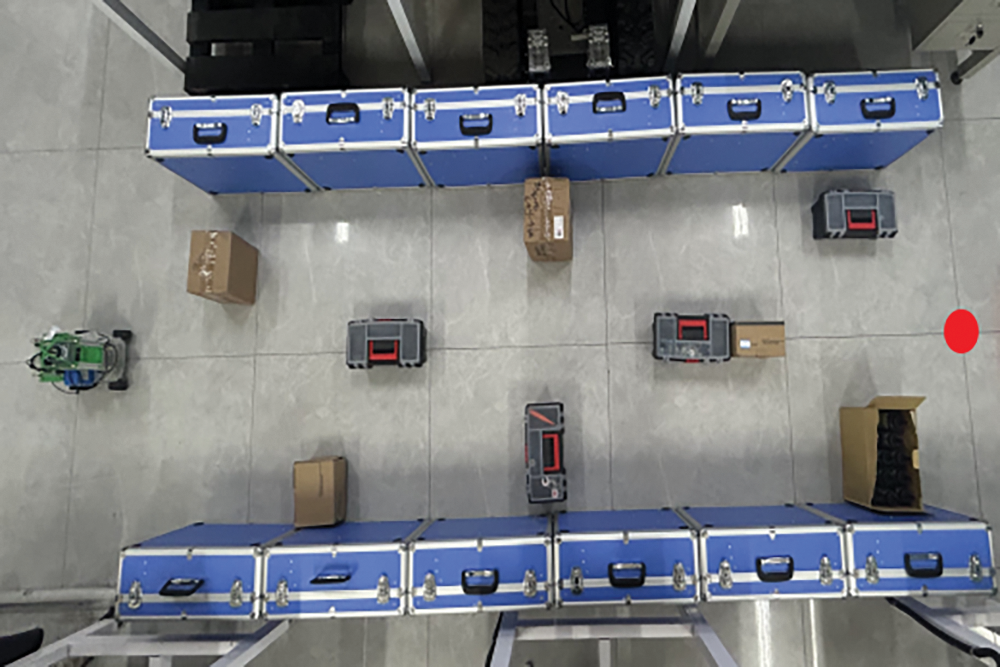
Figure 15: Experimenting with real scenarios

In this paper, Mid-360 3D LiDAR combined with the Fast-lio2 algorithm is used to reconstruct the real scene in Fig. 15 in 3D, and the specific effect of the established point cloud map is shown in Fig. 16a. Because of the limited arithmetic power of the ROS main control board used in this paper, it is not possible to navigate in the point cloud map, so Octomap is used to convert the established point cloud map into a 2D raster map and save it. The navigation system was constructed based on the Movebase framework, and the I-BJPS algorithm was successfully deployed and compiled. During the navigation process, the saved raster map was loaded, and the coordinates of the target points were released after the algorithm was fully loaded. The planned global path is shown in Fig. 16b, where the thin green solid line indicates the global path planned by the algorithm, the green dashed line indicates the boundary line that matches the obstacles at the map boundaries, and the planning time for the global path is 0.129 s, and the path length is 5.18 m. It can be seen from Fig. 17 that the improved I-BJPS algorithm can quickly plan an optimal path that matches the robot’s walking.

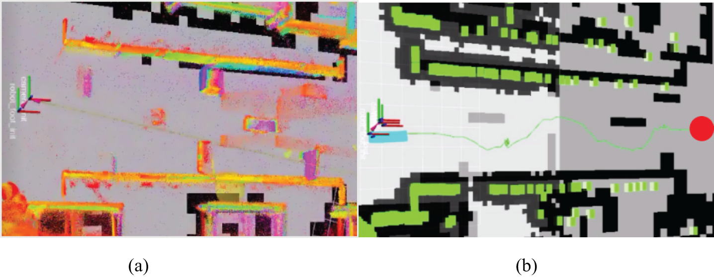
Figure 16: Validation of global path planning validity

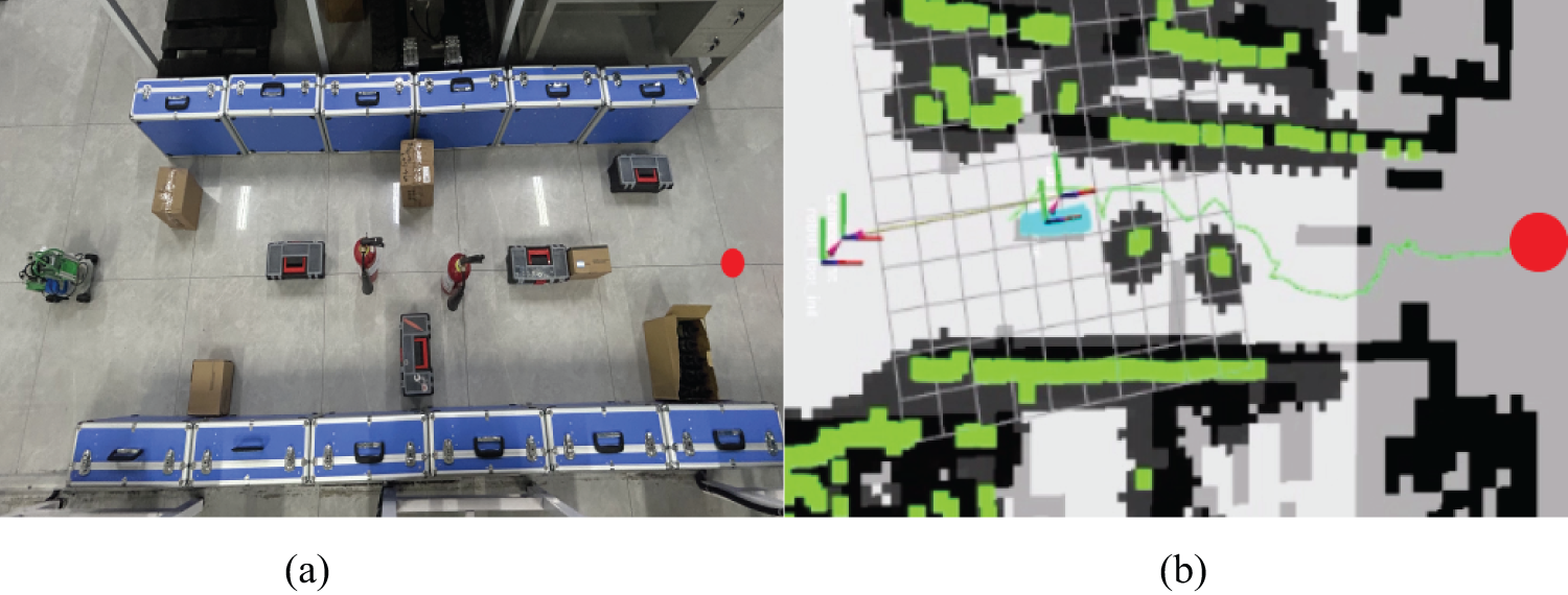
Figure 17: Validation of the effectiveness of local path planning

6  Conclusion

This paper addresses issues in the traditional JPS algorithm for mobile robot path planning, including excessively extended nodes, numerous inflexion points, slow search times, unsmooth paths, and paths that are too close to obstacles. We propose the following improvements to the original BJPS algorithm:

(1) Dynamically defines the weighting factors in the heuristic function and proposes a pruning strategy to eliminate the redundant nodes generated in the planning process effectively. Simulation experiments are carried out under three complex scenarios of 30 × 30, 50 × 50 and 80 × 80 raster maps, and the results indicate that the improved algorithm has higher search efficiency on small-scale maps, while in large-scale maps, performance is significantly improved in all categories. These results show the effectiveness and practicality of the proposed method in different scale environments;

(2) Introducing the second-order Bezier curve to smooth the turning points in the global path and through simulation experiments in the designed 30 × 30 and 50 × 50 raster maps, the results show that the fused path curves are smoother and more in line with the requirements of the robot’s motion trajectory;

(3) By conducting simulation experiments on 30 × 30 raster maps and actual scenario tests with our self-developed experimental platform, the integration of the DWA algorithm accomplished real-time dynamic planning of local paths, enabling effective circumvention of both known and unknown dynamic and static obstacles along the way. The results demonstrated that this algorithmic fusion successfully evaded the known and unknown obstacles on the global path, substantially enhancing the safety of mobile robots during the path-planning phase.

Acknowledgement: First of all, I would like to express my special thanks to my supervisor, Associate Professor Changyong Li, for your guidance and selfless support in the direction of my research. Also, I would like to thank my students in the lab, your advice and encouragement kept me moving forward in my research. In addition, I thank the Xinjiang Uygur Autonomous Region Central Guided Local Science and Technology Development Funds Project for funding and supporting this research. Finally, I am very grateful to the reviewer experts for their valuable suggestions and the editors for their serious responses!

Funding Statement: This study was supported by the Xinjiang Uygur Autonomous Region Central Guided Local Science and Technology Development Fund Project (No. ZYYD2025QY17).

Author Contributions: The authors confirm contribution to the paper as follows: study conception and design: Zhaohui An; data collection: Zhaohui An, Changyong Li, Yong Han, Mengru Niu; analysis and interpretation of results: Zhaohui An, Changyong Li; draft manuscript preparation: Zhaohui An. All authors reviewed the results and approved the final version of the manuscript.

Availability of Data and Materials: Not applicable.

Ethics Approval: Not applicable.

Conflicts of Interest: The authors declare no conflicts of interest to report regarding the present study.

References

1. Liu LX, Wang X, Yang X, Liu HJ, Li JP, Wang PF. Path planning techniques for mobile robots: review and prospect. Expert Syst Appl. 2023;227(4):120254. doi:10.1016/j.eswa.2023.120254. [Google Scholar] [CrossRef]

2. Rafai ANA, Adzhar N, Jaini NI. A review on path planning and obstacle avoidance algorithms for autonomous mobile robots. J Robot. 2022;2022(1):2538220. doi:10.1155/2022/2538220. [Google Scholar] [CrossRef]

3. Hart PE, Nilsson NJ, Raphael B. A formal basis for the heuristic determination of minimum cost paths. IEEE Trans Syst Sci Cybern. 1968;4(2):100–7. doi:10.1109/TSSC.1968.300136. [Google Scholar] [CrossRef]

4. Dijkstra EW. A note on two problems in connexion with graphs. Numeris Mathema. 1959;1(1):269–71. doi:10.1007/BF01386390. [Google Scholar] [CrossRef]

5. Guo J, Xia W, Hu XX, Ma HW. Feedback RRT* algorithm for UAV path planning in a hostile environment. Comput Indust Eng. 2022;174(2):108771. doi:10.1016/j.cie.2022.108771. [Google Scholar] [CrossRef]

6. Lin SW, Liu A, Wang JG, Kong XY. An improved fault-tolerant cultural-PSO with probability for multi-AGV path planning. Expert Syst Appl. 2024;237(21):121510. doi:10.1016/j.eswa.2023.121510. [Google Scholar] [CrossRef]

7. Li GX, Liu C, Wu L, Xiao WS. A mixing algorithm of ACO and ABC for solving path planning of mobile robot. Appl Soft Comput. 2023;148(15):110868. doi:10.1016/j.asoc.2023.110868. [Google Scholar] [CrossRef]

8. Cheng X, Li J, Zheng C, Zhang J, Zhao M. An improved PSO-GWO algorithm with chaos and adaptive inertial weight for robot path planning. Front Neurorobot. 2021;15:770361. doi:10.3389/fnbot.2021.770361. [Google Scholar] [PubMed] [CrossRef]

9. Harabor D, Grastien A. Online graph pruning for pathfinding on grid maps. Proc AAAI Conf Artif Intell. 2011;25(1):1114–9. doi:10.1609/aaai.v25i1.7994. [Google Scholar] [CrossRef]

10. Cai JC, Bai KQ, Li XC, Huang ZL, Liu GZ. Improved mobile robot path planning algorithm based on JPS. Comput Appl Res. 2022;39(7):1985–91. doi:10.19734/j.issn.1001-3695.2021.12.0671. [Google Scholar] [CrossRef]

11. Liu RH, Wang X, Wu D, Xie CY. Improved bidirectional dynamic JPS algorithm for global path planning of mobile robots. Comput Appl Res. 2024;41(4):1117–22. doi:10.19734/j.issn.1001-3695.2023.08.0369. [Google Scholar] [CrossRef]

12. Wei B, Yan H. An improved jump point search path planning algorithm for unstructured environments. Sci Technol Eng. 2021;21(6):2363–70. [Google Scholar]

13. Hou YX, Gao HB, Wang ZJ, Du CS. Path planning for mobile robots based on improved jump point search method. J Combin Mach Tools Autom Process Technol. 2023;3:54–8. doi:10.13462/j.cnki.mmtamt.2023.03.014. [Google Scholar] [CrossRef]

14. Wang Z, Tu HX, Chan SX, Huang CK, Zhao YW. Vision-based initial localization of AGV and path planning with PO-JPS algorithm. Egypt Inform J. 2024;27(2):100527. doi:10.1016/j.eij.2024.100527. [Google Scholar] [CrossRef]

15. Li Y, Zhang J, Liu Y, Zhang Y, Yang M. Design of logistics robot scheduling system and its bidirectional synchronous jump point search algorithm. J Instrum. 2023;44(7):121–32. doi:10.19650/j.cnki.cjsi.J2311272. [Google Scholar] [CrossRef]

16. Feng D, Deng L, Sun T, Liu H, Zhang H. Global path planning based on an improved A* algorithm in ROS. Lect Notes Electr Eng. 2022;799:1134–44. doi:10.1007/978-981-16-5912-6. [Google Scholar] [CrossRef]

17. Vahide B. Path planning of mobile robots in dynamic environment based on analytic geometry and cubic Bézier curve with three shape parameters. Expert Syst Appl. 2023;233(3):120942. doi:10.1016/j.eswa.2023.120942. [Google Scholar] [CrossRef]

18. Li Y, Li J, Zhou W, Yao Q, Nie J, Qi X. Robot path planning navigation for dense planting red jujube orchards based on the joint improved A* and DWA algorithms under laser SLAM. Agriculture. 2022;12(9):1445. doi:10.3390/agriculture12091445. [Google Scholar] [CrossRef]

19. Li Y, Jin R, Xu X, Qian Y, Wang H, Xu S, et al. A mobile robot path planning algorithm based on improved A* algorithm and dynamic window approach. IEEE Access. 2022;10(6):57736–47. doi:10.1109/ACCESS.2022.3179397. [Google Scholar] [CrossRef]

20. Cailian LAO, Peng LI, Yu FENG. Path planning of greenhouse robot based on fusion of improved A* algorithm and dynamic window approach. Transact Chin Soc Agricul Mach. 2021;52(1):14–22. doi:10.6041/j.issn.1000-1298.2021.01.002. [Google Scholar] [CrossRef]