Neural Network Algorithm Based on LVQ for Myocardial Infarction Detection and Localization Using Multi-Lead ECG Data

1  Introduction

Myocardial infarction (MI) is one of the leading causes of death globally among cardiovascular. Cardiovascular diseases are the primary cause of death worldwide [1], with myocardial infarction (MI) being a significant contributing factor. MI involves the necrosis of the heart muscles due to insufficient blood supply [2], being a condition that carries a high risk of mortality and necessitates emergency medical treatment. The early diagnosis and precise localization of developing myocardial infarction play a key role in reducing fatalities and improving prognoses in cardiac patients with various illnesses. ECG is a more common and affordable method for diagnosing MI among existing methods, with the advantages of methodical simplicity in its implementation and cost-effectiveness in use [3–5], when compared with echocardiography [6,7] and coronary angiography [8]. However, interpreting ECG data—especially regarding the location of the necrotic area in the case of a heart attack—remains a challenging and crucial task that requires high accuracy.

Accuracy in identifying the necrotic area in the case of myocardial infarction is critical to choosing appropriate treatment tactics, as mistakes in localization can lead to ineffective treatment and deterioration in the prognosis of cardiac patients with various comorbidities [9,10].

In recent years, machine learning and neural network technologies have been actively implemented in medical diagnostics, offering new opportunities for analyzing the clinically significant parameters of ECG data [11–14]. Despite the successes in this field, most existing methods and approaches that identify MI localization based on ECG data fail to consider the importance of each lead’s individual contribution to the overall picture of cardiac diagnostics. The authors of this article previously developed and proposed a new wearable four-lead ECG apparatus [15] dedicated to the extended monitoring of cardiac activities in a patient’s daily life. The research results revealed that reducing the number of measuring channels to four channels (leads) limits the potential to precisely locate the damaged structure of heart muscles, which was also confirmed by Sun et al. [16]. It is important to note that visualizing ECG data in the context of myocardial infarction based on a four-lead system can result in a reduction in the informative value of the data and failure to detect significant ischemic changes in certain parts of the myocardium, thereby lowering the diagnostic accuracy and the overall efficiency of the system. Considering these limitations, the authors decided to develop an approach based on machine learning methods for the analysis of ECG data, developing a 12-lead ECG system that provides a complete and more detailed view of heart muscle condition, which is critical for accurately detecting the localization of myocardial infarction-associated damage. The accuracy and efficiency of the MI localization system can be enhanced by implementing effective machine learning methods and approaches after their validation on multi-channel recordings of ECG data. According to numerous studies [17–19], existing approaches to identify the localization of necrosis areas in MI require only the manual selection of the ECG lead by a cardiologist, or necessitate that all 12-lead ECG data are processed the same way without any decision rules, which can result in the redundant processing of information. This research proposes a neural network approach based on the learning vector quantization (LVQ) algorithm, enabling us to consider the limitations of the methods mentioned above. It enables high-accuracy MI localization, as neural network-based analysis of the ECG data is performed for each lead in the 12-channel system, which facilitates the accurate localization of MI. For this study, data for neural network-based analysis of ECG data from 12-lead systems were obtained from the verified Physikalisch-Technische Bundesanstalt (PTB) database. The results obtained can serve as a basis for the development of wearable devices that monitor patients’ states using a limited number of measuring channels, while also delivering a more accurate diagnosis and timely response to critical conditions. The research and development of machine learning methods based on a 12-lead ECG system is an important step for creating accurate myocardial infarction diagnostics systems that are capable of subsequently functioning within the framework of wearable devices [15,20], which are characterized by an insignificant number of channels.

The key contribution and novelty of this study is the proposal of an improved LVQ-based model for ECG signal classification, which demonstrates high accuracy and stability in diagnosing myocardial infarction.

In recent years, a significant amount of research has been conducted on ECG signal analysis using various machine learning and neural network methods [21]. The most common approaches include the use of convolutional neural networks (CNNs) and recurrent neural networks (RNNs), which have shown high efficiency in classifying ECG signals and diagnosing heart diseases. Also study [22] used ResNet, which is a special convolutional neural network with skip connections. This structure allowed for deeper models with more layers, which was a significant breakthrough in deep learning. The study [23] developed DenseNet and CNN models to classify healthy subjects and patients with 10 classes of myocardial infarction based on the location of the myocardial lesion. However, most of these methods have many limitations that hinder their practical application.

One of the main limitations is their lack of robustness to noise in data, which is often encountered in real-world settings. Noise caused by patient movement or other external factors can reduce the classification accuracy, especially if the used data pre-processing methods are ineffective. Many existing studies involve pre-filtering the signals, but they do not always cope successfully with different types of noise, making the model vulnerable to data variability.

Another limitation is the use of the Euclidean distance or other simple metrics to measure the similarity of signals, which may be ineffective when analyzing non-stationary data such as ECG signals. Such metrics cannot always correctly account for dynamic changes in the shape of signals, which leads to losses in classification accuracy. Modern studies have noted the need for more flexible approaches to measuring similarity that can account for temporal and amplitude changes in signals.

In addition, much of the existing literature has focused on complex deep neural network architectures that have high computational resource requirements. This limits their application in real-world conditions, especially on the mobile and portable devices used in the context of health monitoring. In this regard, there is a need to develop lighter models that can effectively operate in environments with limited resources.

Our study seeks to overcome these limitations through the use of an LVQ model, which combines high classification stability with relative simplicity and resistance to noise, thus making it suitable for conditions characterized by limited computational resources and high data variability, as is common in real-world cardiology applications.

This study contributes to the field by proposing an advanced model based on LVQ (Learning Vector Quantization) for ECG signal classification, achieving high accuracy and stability in myocardial infarction diagnosis, particularly under limited computational resources. This approach addresses existing gaps, including the individual contributions of each lead, enhancing localization precision and noise resilience.

The structure of the article is as follows. Section 2 is dedicated to describing the research methodology, including data preprocessing steps, the selection of the LVQ model, its architecture, and the training and testing procedures. Section 3 presents the experimental results, including a comparative analysis with state-of-the-art methods and key performance metrics. Section 4 offers a discussion of the results, their interpretation in the context of existing literature, and the identified limitations of the study.

2  Materials and Methods

2.1 Data Collection and Processing

The ECG data used in this study were obtained from the PTB Diagnostic ECG Database, provided by the National Metrology Institute of Germany (PTB) and accessible through PhysioNet. This publicly available database contains 549 recordings from 290 participants, including both healthy individuals and patients with various cardiovascular diseases. The dataset is available for use under the Open Data Commons Attribution License v1.0 [24]. The ECG data applied in this research were collected using a prototype 16-lead recorder, including 14 channels for recording ECG signals, 1 channel for breath measurement, and 1 channel for line voltage measurements. The data set includes 549 recordings from 290 subjects aged 17 to 87 years with various cardiovascular conditions. Each subject provided between 1 and 5 recordings, with each recording containing 15 signals (12 standard ECG leads and 3 Frank leads). The data were digitized at a sample rate of 1000 Hz and a 16-bit resolution. We obtained ECG recordings of 56 healthy people and 146 patients with different forms of myocardial infarction; in some patient folders, there were several ECG recordings. In total, we managed to obtain 79 ECG recordings from healthy individuals and 366 ECG recordings from patients diagnosed with MI.

2.2 Inclusion and Exclusion Criteria

This study included participants over 18 years of age with a confirmed diagnosis of myocardial infarction, as well as healthy individuals who had undergone a preliminary examination to exclude cardiac pathologies. Patients with high-quality ECG signal recordings were also selected, which ensured the accuracy of subsequent data processing.

Individuals with other cardiovascular diseases that could affect the shape of the ECG signals (e.g., arrhythmia or heart failure), as well as patients with chronic or acute diseases affecting cardiac function (e.g., severe hypertension) were excluded from the study. ECG recordings with a high noise level that could not be eliminated at the pre-processing stage were also excluded.

2.3 Data Pre-Processing

Signals from a standard 12-lead ECG system were extracted for each patient. Data were preliminarily processed as follows: Data pre-processing included standardization using StandardScaler, ensuring unification of the amplitude characteristics of the ECG signals. The signals were brought to a single length (500 samples), by trimming or padding with zeros, in order to eliminate variability. To improve signal quality and remove noise, bandpass filtering was applied. Specifically, a 4th-order Butterworth filter with a passband of 0.5 Hz to 40 Hz was used to eliminate baseline wander and high-frequency noise. For class balancing, equal samples of healthy participants and patients with myocardial infarction were used, which minimized model bias. The data set was divided into training and testing sets in a ratio of 80:20, with preliminary random mixing. After filtering, approximately 15% of noisy signals were excluded, which improved the data quality and classification accuracy.

As a result, the total dataset consisted of 445 ECG recordings, including 79 from healthy individuals and 366 from patients with myocardial infarction. The training set comprised 356 recordings (80% of the total), while the testing set included 89 recordings (20% of the total). This ensured a robust distribution of data for effective model training and evaluation.

2.4 Training and Testing Preparation

The data were clustered into training and testing sets (80% and 20%, respectively). This split provided a sufficient data volume for the training of models and their subsequent testing on an independent data set. Category labels (healthy or MI diagnosed) were converted into a one-hot encoding format, which is necessary for effective neural network learning. Such a detailed approach to data preparation provides a high-quality input data for the subsequent machine learning training process, as well as improving the prediction accuracy.

The characteristics of the output of the ECG data were described through double descriptive analysis based on parametric and non-parametric statistics. The data are described with the average M and standard deviation σ, and are presented as M ± Std. Data with a non-normal distribution are described with the median Ме and quartiles Q1 and Q3, and are presented as Me [Q1; Q3]. Data with a non-normal distribution were assessed with indicators of asymmetry (As), excess kurtosis (Ek), and Kolmogorov–Smirnov–Lilliefors criteria statistics, when counting more than 50 signals. The data were considered statistically significant at p < 0.05. Table 1 illustrates the characteristics of the ECG signal obtained from the standard lead II, comparing a healthy patient with one presenting a myocardial infarction.

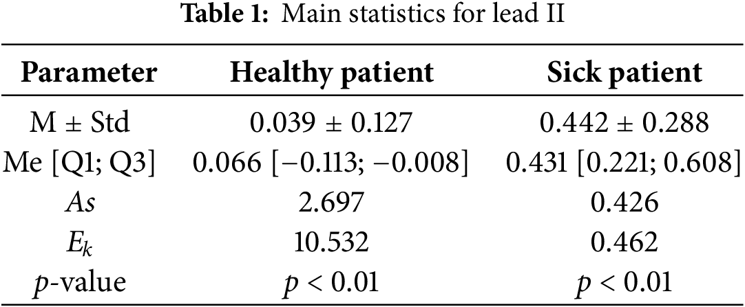
Table 1 indicates a minor discrepancy between the median (Me) and the average (M) of the analyzed data. However, the kurtosis (Ek) and asymmetry (As) metrics illustrate the peak and right-sided asymmetry in the distribution series, supported by the p-value from the Kolmogorov–Smirnov–Lilliefors criteria; if the p-value of this criteria is less than the threshold, it confirms that the probabilistic distribution of the ECG data model is different from the Gaussian distribution. In the given situation, all values of the indicators for the two ECG data sets under examination presented distinctions among themselves, which can be explained by specific changes and ongoing bioelectric processes in the heart muscle in the context of myocardial infarction.

The method is based on the idea that heart bioelectrical signals have a natural distribution on the surface of the body and can be registered (allocated), intensified, and then recorded as a characteristic curve (i.e., via ECG). This was successfully achieved for the first time by W. Einthowen in 1903, who designated the ECG teeth with the following consecutive letters of the Latin alphabet: P, Q, R, S, and T. In particular, ECG allows a graphical representation of the electrophysiological processes occurring in the myocardium to be obtained.

The heart functions (beats) by electrical impulse, which generates its own pacemaker. Anatomically speaking, this pacemaker is located on the right atrium, along with a collection of empty veins in the sinus node. The excitation pulses that arise from it are called “sinusoidal pulses”. The sinus node generates electrical impulses which arouse the myocardial tissue by spreading through the conductive system. As a result of the electrical activity of myocardial tissue, the heart creates a periodically changing electrical field around itself. Electrodes placed on the skin perceive the changes in this field and transfer them to an electrocardiograph.

Fig. 1 illustrates the ECG (electrocardiogram) waveform, highlighting the QRST complex (Q, R, S, and T waves), which are essential for diagnosing cardiac conditions.

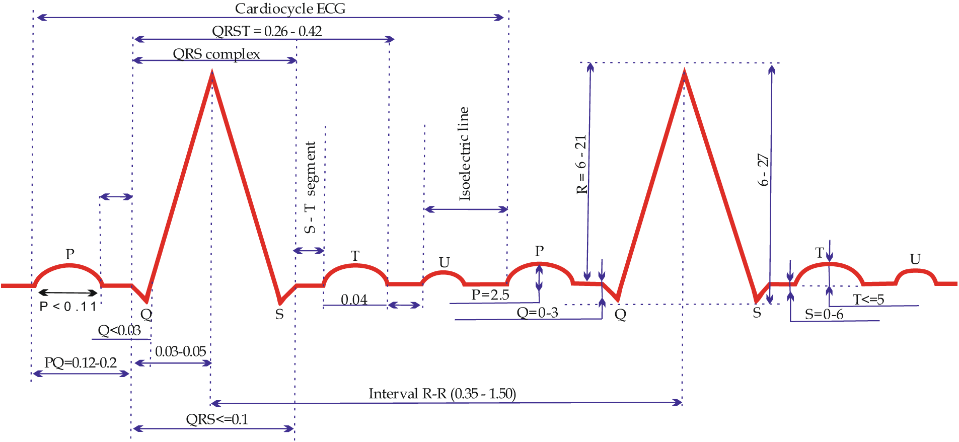
Figure 1: Waves and intervals of a normal ECG

Apart from registering the teeth vertically, the time is recorded on the ECG vertically, during which the impulse passes through certain parts of the heart. A segment of the cardiogram, measured by its duration in time (s), is called an interval. An electric excitation pulse occurs in the sinus node (which is not registered on the ECG), spreads through the atrium (wave P on the ECG), and travels through the atrioventricular (AV) node (see Figs. 1 and 2). A physiological pulse delay (speed contraction in its performance) occurs in the atrioventricular (AV) node; thus, on the ECG, the area between P and Q waves (PQ segment) is represented by a straight line known as the isoelectric line (isoline). Further, the electrical impulse reache Myocardial infarction (MI) is one of the leading causes of death globally among cardiovascular s the ventricular conduction pathways offered by the bundle of His and Purkinje fibers (see Fig. 1) and arouses the ventricular myocardium. This process is indicated by the formation of a ventricular complex; specifically, the QRS complex (see Fig. 2). Engulfing the ventricles with arousal, the electric excitation impulse fades and, simultaneously, repolarization processes occur (represented by the ST segment and T wave in the ECG).

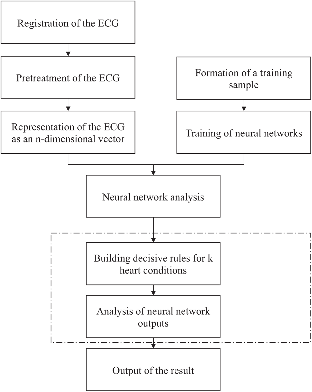
Figure 2: Algorithm for neural network-based analysis of electrocardiographic signals

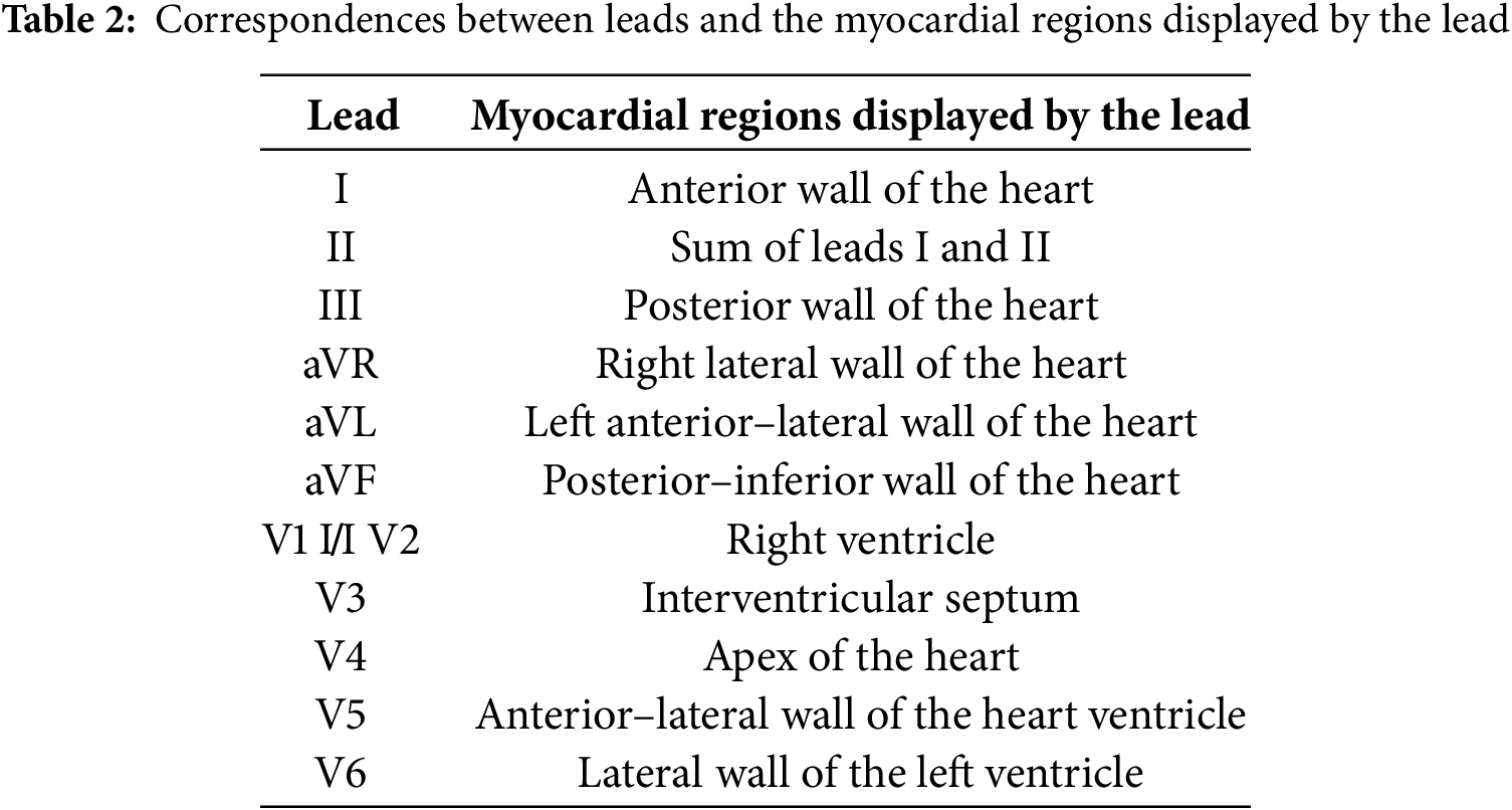
The genesis of the ECG is thus determined by the depolarization (excitation) and repolarization (relaxation and restoration of its resting state) of myocardium cells. Each of the 12 standard leads makes it possible to register the changes in the electrical activity of certain parts of the heart. Table 2 presents information about these parts and their conditions, with respect to the standard leads.

2.5 Learning Vector Quantization (LVQ) Algorithm

The learning vector quantization (LVQ) algorithm is one of the machine learning methods dedicated to classifying the data based on prototypes. In this research, LVQ was used for the classification of ECG data in order to identify myocardial infarction (MI). This algorithm was selected due to its ability to effectively process multi-dimensional data and provide a high accuracy of classification. To achieve high performance in diagnosing and localizing myocardial infarction, a Learning Vector Quantization (LVQ) model was selected. This method was chosen for its ability to efficiently process multidimensional data while maintaining robustness to noise. Unlike more complex deep learning architectures such as CNNs and RNNs, LVQ strikes a balance between accuracy and computational efficiency, making it particularly suitable for applications in resource-constrained environments.

The model’s structure is based on using a separate network for each heart condition, allowing it to account for the specific characteristics of each class. Training is conducted on preprocessed data, which includes normalization, noise filtering, and class balancing. Standard metrics, such as accuracy, recall, and F1 Score, were employed to evaluate the model’s performance, enabling an objective comparison of the proposed approach with state-of-the-art methods.

Thus, the use of LVQ not only demonstrates stable and high accuracy in ECG signal classification but also opens up possibilities for its application in portable devices and monitoring systems, where limited computational resources remain a critical factor.

An electro-cardiosignal (ECS) is registered and pre-processed, after which it is converted into an n-dimensional vector. Then, m such vectors are created, which reflect various conditions of the heart, and are compared with the registered ECS, following which it can be determined whether the signal enters the threshold range for any particular cardiac condition. Further, a neural network analysis is conducted, through which additional vectors for reference data are created. Based on the formulated decision rules, an analysis is conducted and the system identifies one of the k possible cardiac conditions. Furthermore, the LVQ neural network is used for neural network-based analysis of the ECS, which is a development of the Kohonen network structure and provides the opportunity to train with a teacher.

For neural network-based analysis of n-dimensional vectors, a registered electro-cardio signal, a K × L (L: number of leads) neural network is developed to analyze each of the k heart conditions for each lead. Decision rules are then formulated based on direct and reciprocal signs of topical diagnostics for each of the k conditions of the heart. The findings relating to one of the k conditions are obtained by choosing the heart condition for which the maximum number of signs are detected.

Fig. 2 illustrates the algorithm for the neural network-based analysis of cardiac conditions.

Fig. 2 shows the scheme followed to form a diagnostic conclusion regarding the patient’s heart condition relating to one of the two heart conditions (healthy state and myocardial infarction of anterior and anteroposterior localization), considering the results of the initial ECG neural network-based analysis.

Fig. 3 presents a method for the neural network-based analysis of heart conditions, including the following processes (see Fig. 2): “Registration of the ECG signals”, “Pre-processing of the ECG signals”, “Representation of the ECG signals as an n-dimensional vector”, “Formation of a training sample”, “Training of neural networks”, “Neural network analysis”, “Building decision rules for k heart conditions”, “Analysis of neural network outputs”, and “Output of the result”.

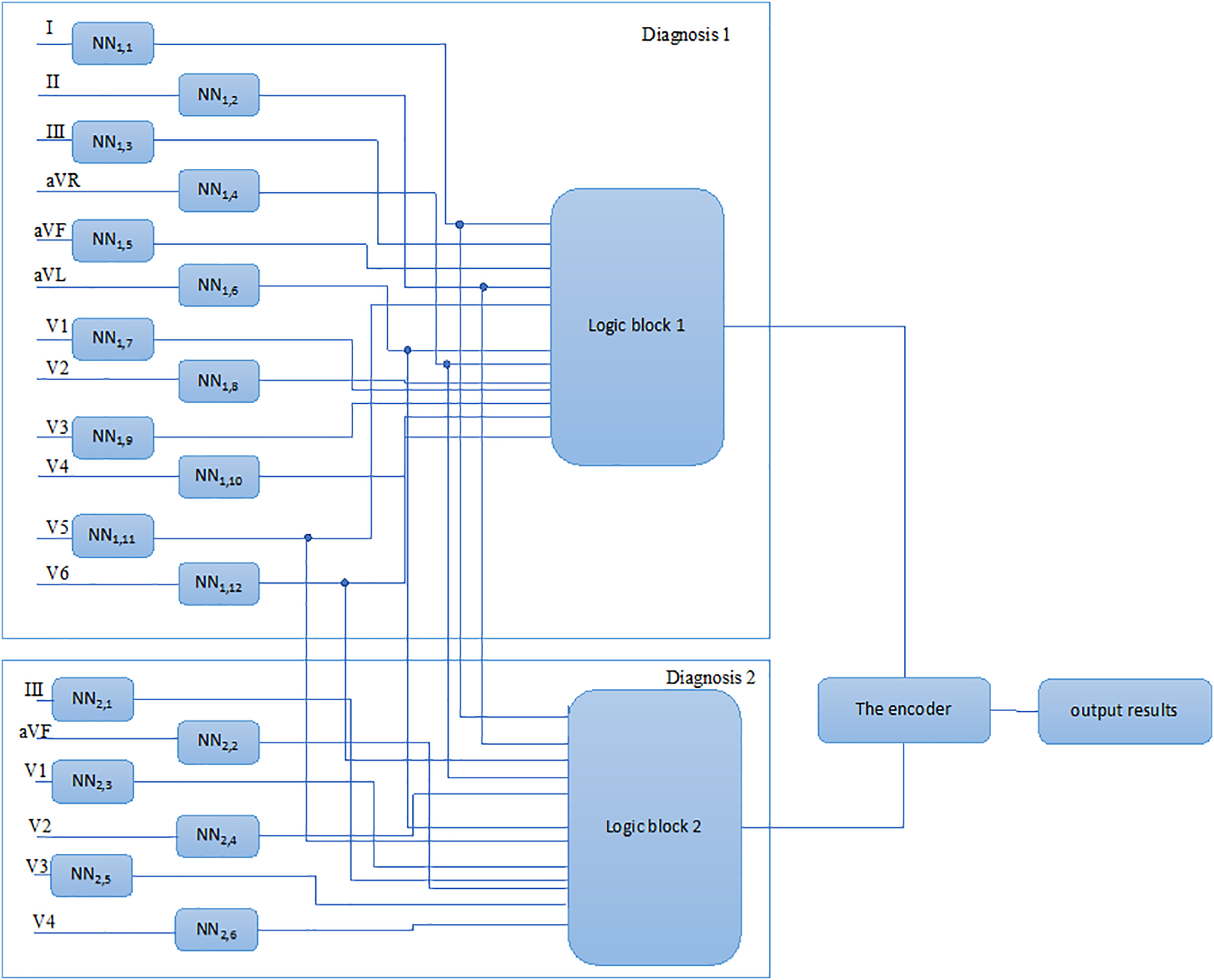
Figure 3: Method for the neural network-based analysis of heart conditions

In the ECG registration stage, the ECG device output and registration are executed utilizing the ECG registration device. During registration of the ECG device, the following problems must be addressed:

–   The electrical relationship between electrodes and skin tissue at the location of the electrodes;

–   The patient’s electrical safety;

–   Analogous filtration and enhancement of the ECG device;

–   Sampling and digitalization of the ECG device;

–   Interfacing of the ECG registration device with the computer.

After registration, the digitized ECG data are sent to the computer.

At the stage of the ECG pre-processing, the following issues are addressed:

–   Digital filtering, including noise suppression and the removal of artifacts. Utilizing digital filters, irregular beats from registered ECG series are removed, highlighting features of the ECG amplitudes of the P, Q, R, S, and T waves and the values of the midpoints between the P and Q waves and S and T waves;

–   Obtaining coefficient values after performing Fourier and wavelet transforms.

Following the pre-processing stage, data that characterize the features of the registered ECG signals are acquired, which are required for the construction of an n-dimensional vector.

Representation of the ECG signals as an n-dimensional vector: In this stage, the n-dimensional vector is formed using the obtained values. Two n-dimensional vector formation variants can be distinguished. In the first case, the values of the n-dimensional vector are characteristic features of the ECG data, including amplitudes of P, Q, R, and S waves and the values of the midpoints between P and Q waves and S and T waves; in the second case, the values of the n-dimensional vector are the values of coefficients obtained after performing Fourier and wavelet transforms.

The training samples were formed based on the inclusion of each condition in the heart ECG database for each lead involved, with the following steps:

1.   An analysis of the registered ECG signals is conducted by an experienced cardiologist and, according to the analysis results, the registered ECG signals are each associated with one of the k conditions of the heart.

2.   Statistical processing is performed for each of the k conditions in the heart ECG database, with the following stipulations:

The number of ECG signals for one heart condition must not be less than 50;

–   The number of ECG signals for one heart condition can be split into two equal samples;

–   A null hypothesis is introduced, stating that the considered samples all belong to one of the general populations;

–   The parameters of the t-criterion are calculated [7];

–   Under the condition tfact > ttable, the correlation coefficient is regarded as substantial, and the null hypothesis that the considered samples belong to the same general population is accepted.

Split the number of ECG signals for one heart condition into two parts (training and testing) in a ratio of 4:1.

Split the number of ECG signals for one heart condition into two segments (noise-free and noisy) in a ratio of 3:1.

ECG noise suppression.

Use the obtained ECG signals (noise-free and noisy) to train k neural networks.

Use the test ECG signals to validate the k trained neural networks.

2.6 Forming a Training Sample for Cardiac Cycle Segment Analysis

This step has definite value as, when low-quality information is present in the training data set, either the neural network will be unable to successfully train or the quality of the trained neural network will be inadequate. To form a training set with the aim of neural network training, it is necessary to complete all the steps presented in the “Pre-processing of the ECG signals” block described above, as well as the following:

(1)   Ensuring that the number of neural network inputs and the number of components in the training data set vectors correspond:

Let x be the isolated cardiac cycle’s component vector, nx is the number of components in the vector x, k is the coordinate vector of the vector components, and n is the number of neural network inputs. n and nx must correspond in neural network training. The parameter n characterizes the neural network’s structure with a certain value (e.g., 150). The value of the parameter nx, which varies for every cardiac cycle ECG, is established with the isolation of a cardiac cycle.

A modified vector of components of the isolated cardiac cycle х′ with length n must be obtained. The stated problem relates to the task of interpolation, which relies on the restoration of intermediate components using known “nodal” values.

As the known nodal values are equidistant, it is advisable to carry out interpolation using Newton polynomials.

In this study, three-node interpolation is used to ensure the best performance, in which the intermediate values are represented by xji and are calculated according to the following formula:

(1)

Therefore, the correspondence of the number of components in the training data set with the number of neural network inputs is ensured.

(2)   Scaling the components of the training data set vectors: For high-quality training of the LVQ neural network, it is necessary to scale the vector components of the training data set. The proposed scaling range is [−1, 1]. Let x be the vector components for an isolated cardiac cycle of the ECG, and xmax be the absolute value of the largest (positive or negative) component of the vector x. Hence, component i of the vector x is scaled according to the following formula:

(2)

(3)   Introducing redundancy into the training set, including noise and time shift: It is beneficial to introduce redundancy into the training set in settings with limited training data. Therefore, each vector xh in the training data set is duplicated R times, where R is the redundancy ratio. Next, the noise vector for the new training data set is identified. Adding vector noise into a training set characterized by redundancy is one of the most effective ways to tackle the issue of “dead” neurons. A noise operation involves the distortion of the value of the vector’s components by adding a random variable Rnd, which is calculated using the following formula:

(3)

where F is the degree of noise (in percentage) and Sind is the value that defines the sign of the calculated value Rnd.

In addition to the noise vector operation on the training set, we propose to apply an additional action—namely, a “time shift”—in which the components of a vector in the training data are shifted by a random value to the left or right in the time axis. These actions are assumed to minimize the number of “dead” and untrained neurons, with the aim of increasing the general capability of the trained neural network.

(4)   Shuffling the vectors in the training set: As a result of prior activities, the training set contains an ordered set of training vectors, which means that all training vectors from a given class follow each other sequentially. This leads to the fact that, in the first epoch of training, the first class is disproportionately represented, thus affecting most of the neurons. Consequently, the neural networks may be trained poorly on data relating to other classes.

The algorithm used to shuffle the training data is straightforward. Let p be the number of vectors in the training set. The algorithm implementation involves preparing a vector that contains new indices for the training set vectors. Each index is defined as a random number within the range of 1 to p; furthermore, indices cannot be duplicated. Then, shuffling of the vectors in the training set is performed in a manner corresponding with the obtained indices. Upon concluding the preparation of the training set, training of the LVQ model is performed.

2.7 Training Neural Networks

In this process, k × L (L, number of leads) neural networks are trained, each of which uses its “own” database and is obtained by completing the previous steps. The adaptation of the LVQ neural network structure parameters for ECG analysis involves modifying the following neural network parameters:

Input vector dimensionality;

The number of neurons in the competitive layer;

The number of output layers.

The paradigm of neural network-based analysis involves ECG sampling, identifying signs of MI from the ECG data, processing them in a neural network, and classifying the heart condition.

2.8 Neural Network-Based Analysis of Electro-Cardio Signals for MI Diagnostics

As mentioned earlier, MI is identified by six main signs, where each signal appears in a certain segment. This approach is implemented as an amplitude–time analysis.

Identifying the information parameters of the ECG signals involves detecting the ascending and descending intervals and consistency of the ECG signals, fixing the fracture points and the amplitude values at these points, and determining the duration of the identified intervals. The detected amplitude–time parameters are compared with the ECG signs of MI in the amplitude–time domain. The heart’s condition is assessed through amplitude–time analysis of the electrical cardiac activity, in order to detect signs of myocardial infarction. Meanwhile, the comparison results are presented alongside an evaluation of the heart’s condition. This approach serves as the foundation for the proposed neural network-based analysis method, which means that neural networks are created for MI signs for each of the 12 standard leads, which means that each model is specifically targeted at finding a certain signal on a certain lead.

Our LVQ neural network was used for analysis of the ECG signals in each of the 12 common leads (see Fig. 4). The initial analog electro-cardio signal (ECG signal in the 12 common leads) was digitized in accordance with the SCP-ECG standard for swapping digited ECG signals, and is presented in the form of 500 counts on one cardiac cycle.

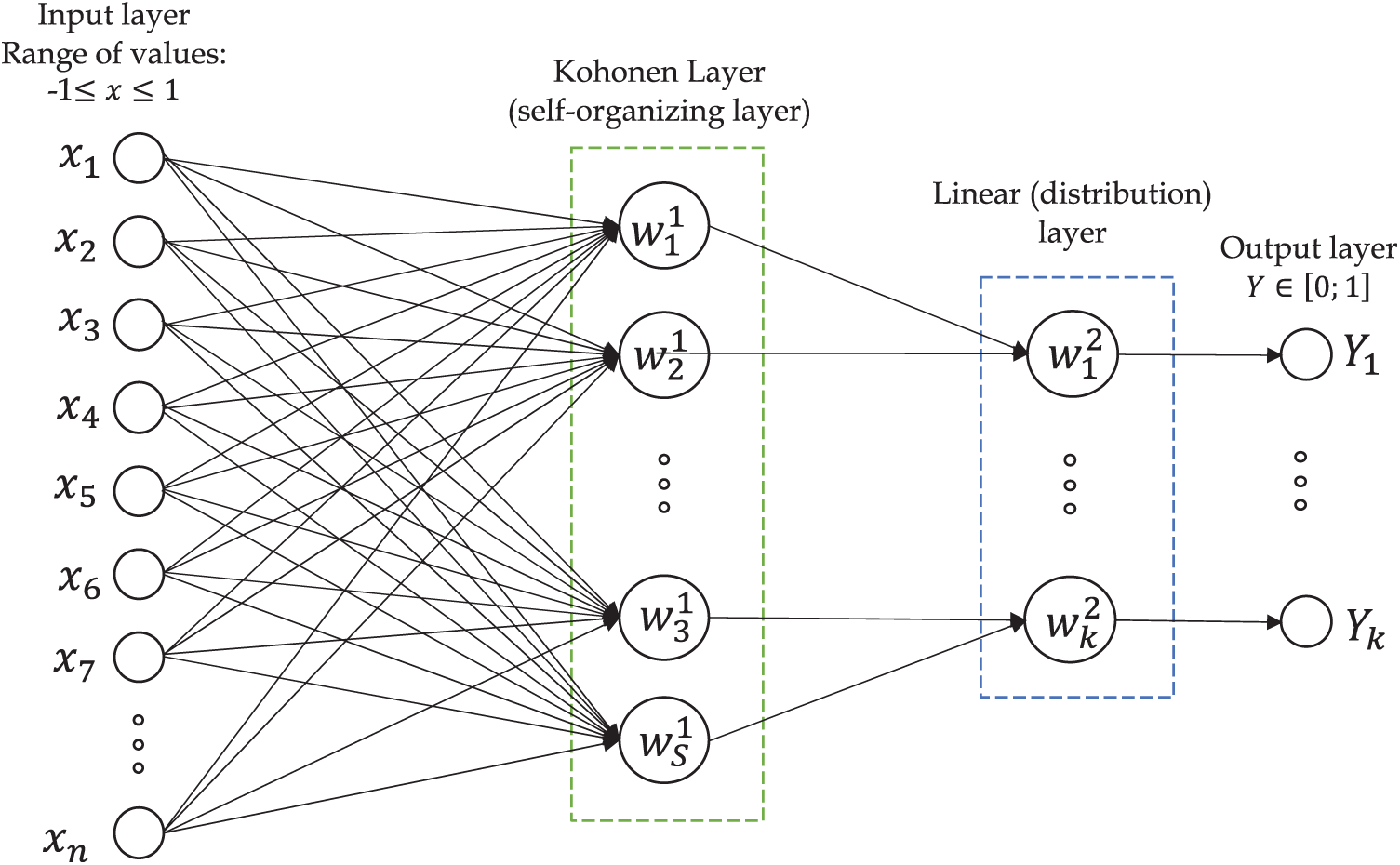
Figure 4: LVQ NN scheme for diagnosis of MI

The isolation of one cardiac cycle is a distinctive feature, as one cardiac cycle is sufficient for the detection of MI.

The count values for one ECG cardiac cycle are used as an input vector хh for the LVQ NN (see Fig. 5).

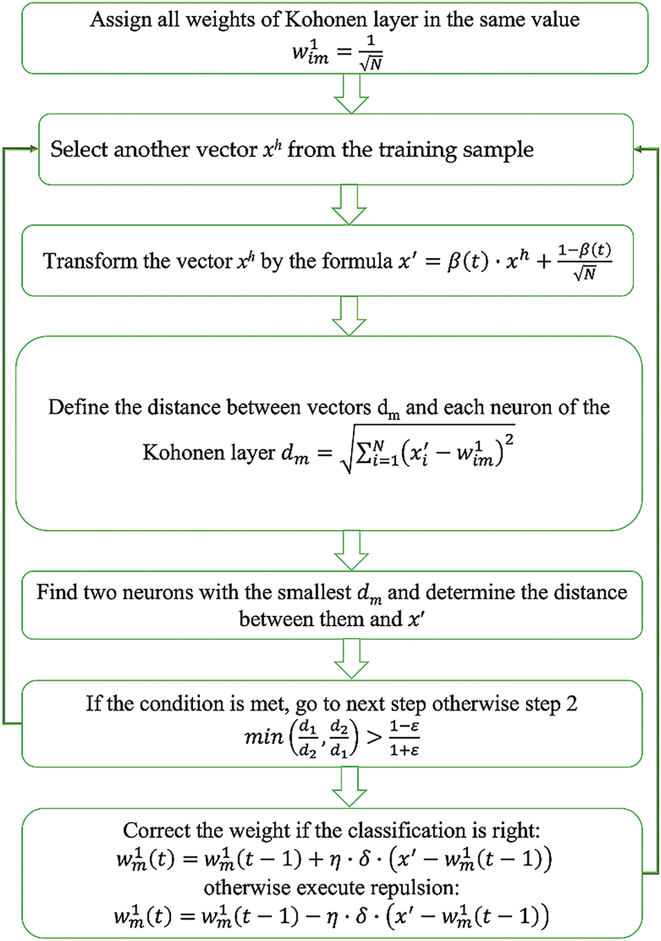
Figure 5: The scheme of the CCLVQ3 training algorithm

The dimension of the input vector is defined by the SCP-ECG standard for exchanging digitized ECG signals: .

The following formula defines the LVQ NN output value:

(4)

where xi is the ith element of the input vector; is the ith element of the weight vector for the competitive layer m; is the jth element of the weight vector for the linear layer k; is the transmission function of the competitive layer, which identifies the winning neuron; is the linear function for activating the neurons in the output layer; is the dimension of the input layer; is the number of neurons in the competitive layer; and is the value of the kth output of the NN.

During the analysis of the input data, the total Euclidean distance should be minimized, as follows:

(5)

where h is the number of input data and is the disease class, corresponding to the vector .

From expression Eq. (2), the problem of locating the minimum value of D is equivalent to searching for the maximum expression:

(6)

The number of neurons in the Kohonen layer corresponds to the number of clusters used to split the input data. The following formula is used to identify this value:

(7)

where α is the number of clusters relating to one class of diseases.

Training of the LVQ NN for each lead is performed after setting the parameters. The aim of training the NN during ECG analysis is to order the neurons (selection of the values of their weights) that minimize the value of expected distortions, assessed according to the approximate error between the input vector and the values of winning-neuron weights in a competitive activity. This error (or recognition error) can be defined as follows:

(8)

where p is the size of the input vector and is the weight vector of the winning neuron in the presence of the vector .

The criteria for finishing the NN training process is satisfaction of the condition < ε, where ε is an error threshold defined by the user before training (e.g., ε = 0.01).

The “convex combination” method was used to training the LVQ neural networks for ECG analysis. The LVQ neural network training algorithm is executed as follows:

(1)   The CCLVQ3 training algorithm is executed as follows:The same initial value is assigned for all weights of the competitive layer, according to the formula:

(9)

(2)   xh is another vector is selected from the training sample.

(3)   The vector components for xh are transformed according to the following formula:

(10)

where t is the number of training epochs and β(t) is a monotonically ascending function, which varies from 0 to 1 during training. If it is equal to zero, the xh vector components are transformed according to Eq. (9).

(4)   The Euclidean distance between the vector x and each neuron of the competitive layer is defined by the following formula:

(11)

where x is the modified training vector, and is the vector of weights for the mth neuron.

(5)   Two neurons are defined—namely, those closest to the vector x—and the Euclidean distances d1 and d2 between these two neurons and the vector x are calculated.

(6)   The execution condition is defined as follows:

(12)

where d1 is the distance from xh to the first winning neuron; d2 is the distance from xh to the second winning neuron; and ε is the error threshold, which can be interpreted as width of the window that the training vector xh should enter. The value of ε is selected in the range of 0.2–0.3.

(7)   The weights of the determined neurons are changed. Positive correction is executed, according to the following formula, if the classification of x is correct:

where m is the number of winning neurons, δ is a parameter affecting the degree of weight correction (as evidenced by practical experience, the optimal value δ in the case of a negative correction to the weights of neurons is in the range from 0.1 to 0.3), and η is a parameter affecting the speed of the weight-tuning process for the neurons in the competitive layer.

In standard training algorithms (for example, LVQ1), the value of η decreases either in a constant (for example, 0.01) or monotonic manner.

In the CCLVQ3 algorithm, the value of η changes during the training process, from 1 to 0. At the beginning of the training, η is equal to 1. After each training epoch, η is adjusted using the following formula:

(13)

where T is the total number of training epochs. In the first epoch, the weight correction is more significant, and the training algorithm seeks to occupy the maximum number of neurons possible to minimize the number of “dead” neurons. Meanwhile, in the last epoch, insignificant weight corrections are performed, but neuron weights trained in the previous epochs are still refined. In this case, if the first of the found neurons is corrected, the δ parameter will be 1. If the second found neuron is corrected, then the value of δ is selected based on what operation was executed on the first neuron: if a correction was performed, then the value will be 0.1; otherwise, if there is a repulsion, then the value will be 1.

In the case of false classification of the vector x, a negative correction—namely, weight repulsion of the neuron—is executed according to the following formula:

(14)

where δ takes a value of 0.2.

It is worth mentioning that repulsion is not conducted during the first epoch of training.

(8)   If the given training epoch is not the last, then the transition to the next epoch is carried out.

2.9 A Method for Drawing a Diagnostic Conclusion

The formation of decision rules for identifying the parts of the heart and their relevant leads.

Heart attack lesions are known to affect certain parts of the heart (segments), which are reflected by changes in the ECG signals obtained with certain leads. Therefore, each segment of the heart can be compared to a specific combination of MI symptoms in a specific group of leads. The precise selection of leads for analyzing different segments of the heart is a key aspect of cardiac disease diagnostics. The proper identification of which lead is more informative for each heart area can significantly enhance diagnostic accuracy and the efficiency of treatment.

Each lead of the ECG reflects electrical activity in various areas of the heart. Understanding which leads are more informative for analyzing various heart segments can be gained based on the anatomical and electrophysiological features of the heart, as follows: Anterior wall of the heart: Leads V1–V4. These leads register the electrical activity of the anterior surface of the left ventricle.

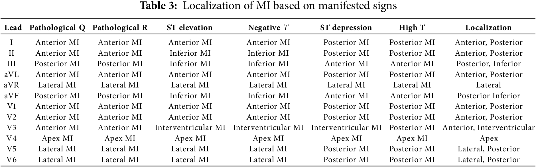
Inferior wall of the heart: Leads II, III, and aVF. These leads record the activity of the lateral surface of the left ventricle. Lateral wall of the heart: Leads I, aVL, V5, and V6. These leads represent the electrical activity of the lateral surface of the left ventricle. Posterior wall of the heart: Even though standard ECG leads do not represent well the posterior wall, the associated changes can be indirectly assessed through leads V1 and V2. The method used to select leads for analysis was based on clinical recommendations and preliminary research results. We used information obtained from a literature review and expert assessments in order to verify the correctness of the selected leads for each area of the heart, including data analyses from clinical trials and research, as well as the use of machine learning methods to assess the significance of each lead. As mentioned earlier, each electrocardiographic lead represents the electrical activity of a certain part of the heart. Thus, according to the presence of MI signs on any lead, we can identify its localization. The principle of decision making is related to the manifested signal of MI which determines its localization. For this purpose, a table for MI decision making was created, as presented in Table 3.

The decision rules for making assumptions regarding the heart’s condition are as follows:

–   Patient is healthy if all segments of the cardiac cycle from all the leads in the results of NNA are assigned to a “healthy” ECG class;

–   In the case of a deviation from the norm, even if one of the segments is identified as pathological, a re-analysis is conducted to assess signs of other cardiac cycles. In the case of confirmation, the patient will be prescribed clinical examination—in particular, troponin testing—or referred for echocardiography testing.

–   The manifestation of signs in more than one segment indicates an obvious pathology. In this case, the diagnostic conclusion is drawn according to the output of the manifested signs.

A neural network analysis was performed concurrently via parallel analysis of the registered ECG signals for each neural network. The output vector of each neural network presents one encoded value, where 1 indicates the network’s positive response in terms of belonging to the kth condition corresponding to the disease; while 0 indicates the signal belonging to the “healthy” class. As a result of the analysis, an array of data consisting of the outputs from a neural network is obtained. The deviations in each MI localization which are not present in all leads determine the analysis rules for the neural network outputs. To formulate decision rules for selection of one of the k − 1 cardiac conditions related to MI, combinations of the presence and absence of direct and reciprocal signs of MI in the ECG signals lead to eight different localizations [12]. The decision rules, forming logical blocks for the eight diagnoses of MI, are as follows:

Lateral MI:

(15)

Inferior MI:

(16)

Anterior MI:

(17)

Infero-Lateral MI:

(18)

Antero-Lateral MI:

(19)

where denote the neural network outputs identifying healthy ECG signals.

A diagnostic conclusion can then be reached depending on the manifested signs of MI, thus representing its localization. For example, identifying the localization of lateral MI is executed according to the following statement:

(20)

where represents the highlighted localization and types of MI, identified as follows:

Furthermore, , represent the manifestations of signs of MI at the corresponding lead g.

Based on the developed MI localization table, depending on the feature, the following logical function for determining the type and localization of MI is obtained:

(21)

where Z is the diagnostic conclusion regarding the type of MI and m is the number of analyzed signs.

2.10 Analysis of Neural Network Output

The data from the neural network outputs are transferred to logical blocks, which are dedicated to identifying relevant cardiac conditions that correspond to the decision rules, and further to a priority encoder, with the aim of identifying the corresponding cardiac conditions. A code number for the entrance line is output by the priority encoder, where a positive entrance signal transmits from the output of one of the k logical blocks of the neural network, as represented in the ECG analysis. An output code is formed when several entrance signals are received simultaneously. When several input signals are received at the same time, an output code is generated corresponding to the input with the highest number, indicating that higher inputs take precedence over lower inputs.

The result of completing this stage of the task is several diagnostic reports on the patient’s heart condition, which is associated with the analyzed ECG data.

2.11 Output of the Result

The numerical results derived from the analysis of the neural network outputs are assigned a verbal description that conveys the diagnostic conclusion regarding the patient’s cardiac status, which is then reported to the user.

3  Results

3.1 Pre-Processing of the Data

In this study, Fourier transforms were used to clean the ECG signals and highlight key diagnostic features. In particular, transforming signals from the time domain to the frequency domain enabled us to detect and remove the noises that are not related to the physiological activity of the heart, such as high-frequency noises and low-frequency oscillations caused by the patient’s movement. Utilizing filters with frequency components improved the signal quality by retaining only those frequencies that are important for ECG analysis, which allowed us to better identify PQRST waves and detect the pathological changes typical of MI.

The ECGs for the leads of healthy and MI-diagnosed patients before Fourier transformation are given below:

Fig. 6 shows the first 5 s of the initial ECG signals for all 12 leads of an MI-diagnosed patient, while Fig. 7 demonstrates similar signals for a healthy patient. Each subgraph presents 1 of the 12 standard leads of the ECG; namely, I, II, III, aVR, aVL, aVF, V1, V2, V3, V4, V5, and V6. In the samples, time is along the X-axis and signal amplitude is on the Y-axis.

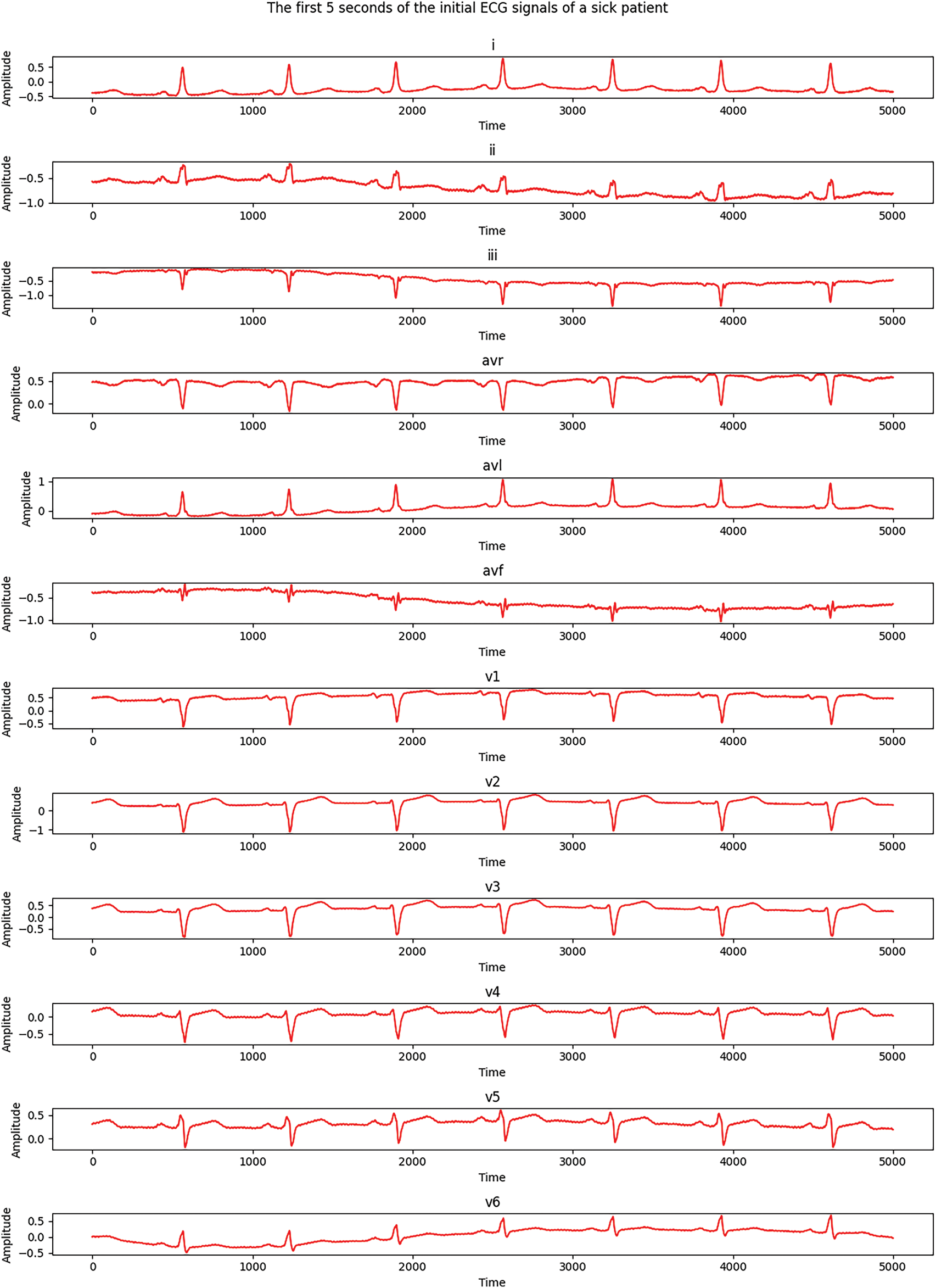
Figure 6: Electrocardiograms of a patient with MI

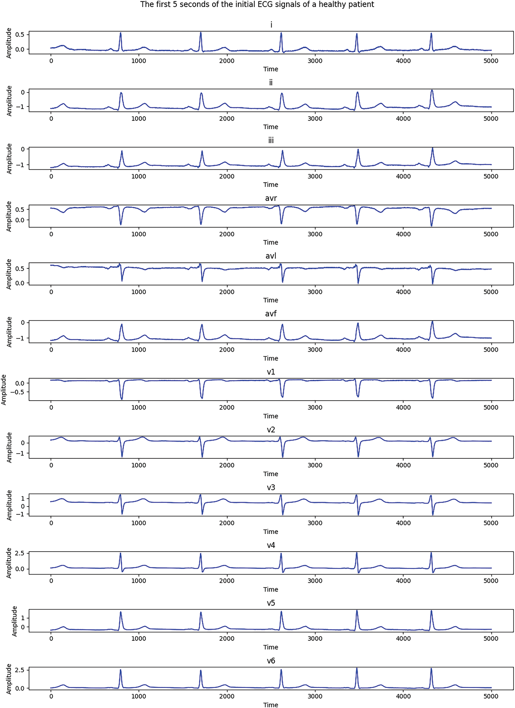
Figure 7: Electrocardiograms of a healthy patient before Fourier transformation

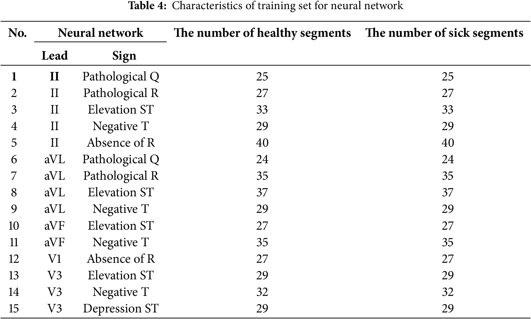
As Figs. 6 and 7 show, there are significant differences between healthy and MI patients. In healthy patients, QRS complexes have a stable and expected amplitude, while the amplitude of QRS complexes in MI patients changes, which is an indicator of myocardial damage. Changes in ST—such as uplift or depression—can be noticed in the ST segments of MI patients, which is a key indicator of myocardial infarction. ST segments in healthy patients are usually located on the isoline.The shape of the T wave can also be changed in MI patients. For example, a T wave inversion can occur, which is an indicator of MI. T waves present a normal shape in healthy patients. Heart rate and rhythm, which might be impaired in a sick patient, can be assessed visually, while the heart rate should be regular and present normal values in a healthy patient.These distinctions help to visually assess a patient’s heart condition and diagnose possible pathological changes which are typical of myocardial infarction. An electrocardiogram of a healthy patient is indicated in red, while that of a patient with MI is marked in blue.A well-formed training set is essential for high-quality neural network training, which is a complicated and laborious process. In this study, a training set was created while ensuring that the same number of training images was used for each analyzed class. A total of 200 ECG patients with a validated diagnosis by cardiologists were examined, of which 52 were healthy and 148 were diagnosed with MI. The number of data elements in the resulting training set is detailed in Table 4.

The following classification metrics were obtained for each of the 12 leads as a result of training and testing neural networks on a sample of 445 ECG recordings (79 healthy subjects and 366 patients with myocardial infarction). The model’s high quality in terms of the detection of MI is evidenced by its classification accuracy of 87%. The classification results for each of the 12 leads are presented in the following Table 5.

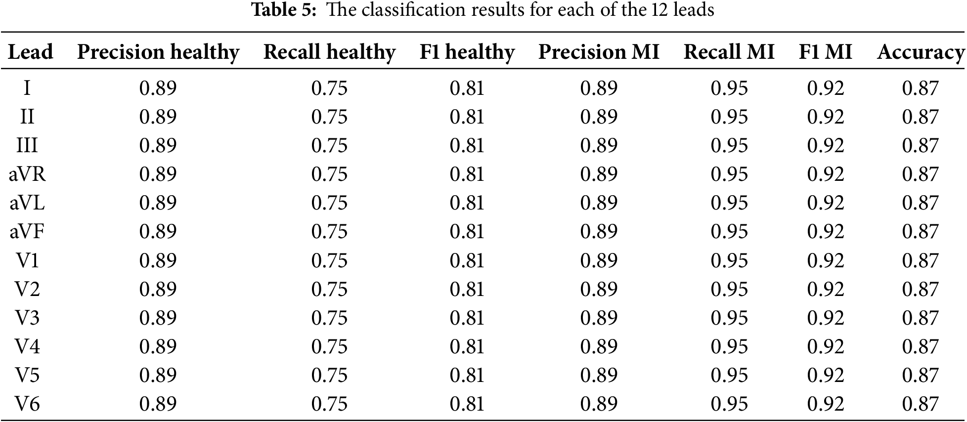
The classification metrics for each of the 12 ECG leads are presented in Table 5. The used metrics include precision, recall, and F1 measure for classification health patients (healthy) and patients with myocardial infarction (MI), as well as overall classification accuracy (accuracy).

The precision and recall values for healthy patients and patients with MI were consistent, with an exceptional classification accuracy of 87% for all leads. This implies that the model exhibits a proportionate outcome in its ability to identify healthy conditions and pathologies associated with myocardial infarction.

The high F1 Scores for both classes confirm that the model can effectively deal with the classification task with all 12 leads of the ECG. These results highlight the reliability of the proposed model for automated MI diagnostics, with the possibility of further improving the model to achieve higher classification scores.

Table 6 provides a comparison of the accuracy and F1 score for each of the 12 ECG leads between the proposed LVQ model, CNN, Logistic Regression, and SVM. This allows for an assessment of the effectiveness of each model in diagnosing myocardial infarction.

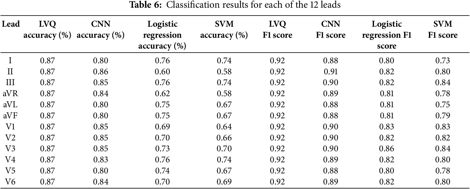
Table 6 presents the accuracy and F1 score values for each of the 12 ECG leads using LVQ, CNN, Logistic Regression, and SVM models. As shown in the table, the LVQ model exhibits consistent performance across all leads, achieving an accuracy of 87% and an F1 score of 0.92 for each channel.

In contrast, the CNN model demonstrates varying accuracy, peaking at 86% on lead II, but dropping to 80% on other channels, such as aVL and aVF. The Logistic Regression and SVM models show greater variability, with accuracy ranging from 60% to 76% for logistic regression and from 58% to 74% for SVM. The observed variability may be attributed to the models’ sensitivity to noise in the data or limitations in capturing complex patterns across certain leads.

A comparative analysis of the accuracy of the models for each lead is shown in Fig. 8.

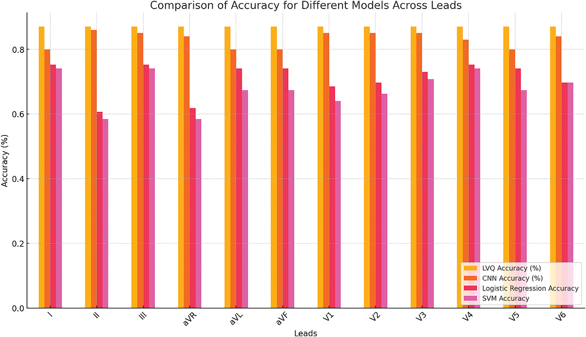
Figure 8: Accuracy comparison under the CCLVQ3 scheme training algorithm

Fig. 8 presents a graph comparing the accuracy of LVQ, CNN, Logistic Regression, and SVM models across all 12 ECG leads. The graph illustrates that the LVQ model maintains stable performance across all leads, while the performance of the CNN model varies. This stability makes LVQ particularly valuable in clinical settings, where consistent and reliable diagnostics are essential, regardless of the input data’s quality or characteristics.

This analysis underscores the importance of selecting a model based on the context of the application: LVQ is well-suited for scenarios where stability and robustness are critical, whereas CNN may be more effective for detecting specific patterns or pathologies in individual leads.

To assess the feasibility of real-time ECG analysis, the classification times for each model were evaluated across all 12 ECG leads. Table 7 presents the classification times, showing that the average time per signal for all models is within the range of 0.000086 to 0.000162 s, confirming their suitability for real-time diagnostic use.

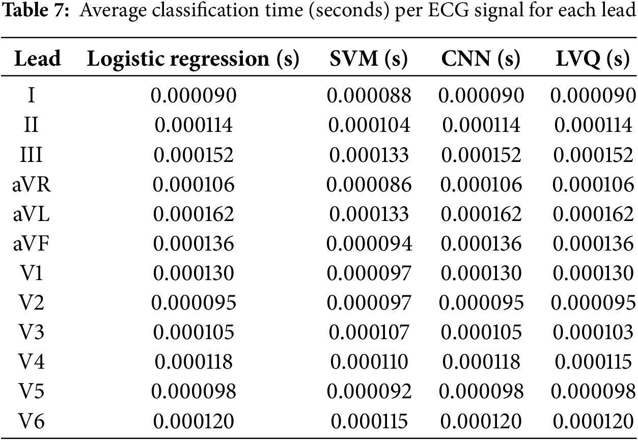
These results demonstrate that the LVQ model, despite its relative simplicity, provides comparable processing times to more computationally intensive models such as CNN. The stability of the classification time across leads is a critical advantage for ensuring real-time diagnostic application.

Fig. 9 complements the data presented in Table 7 by visualizing the classification times for 12 ECG leads across four machine learning models: Logistic Regression, SVM, CNN, and LVQ.

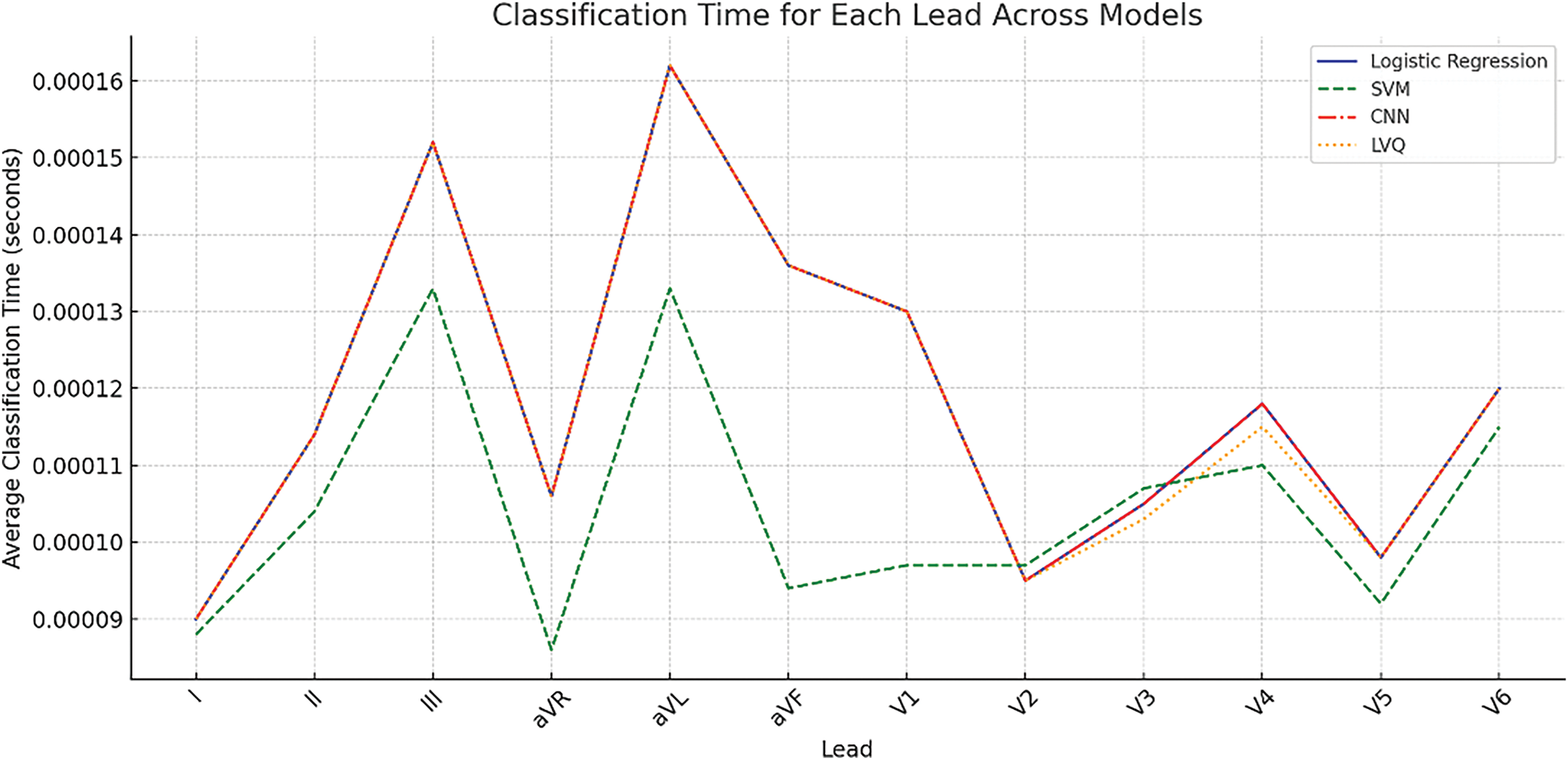
Figure 9: Average classification time per signal for different models across 12 ECG leads

These results highlight that the use of LVQ in particular provides a balance between accuracy and computational speed, reinforcing its suitability for portable cardiac diagnostic systems.

This approach aligns with the broader findings presented in this study, which emphasize the importance of multi-lead ECG analysis for precise myocardial infarction localization while maintaining computational efficiency.

A confusion matrix for each lead was constructed in order to better understand the model’s performance and its capability to differentiate between healthy and pathological conditions. The confusion matrix for lead I is illustrated in Fig. 10.

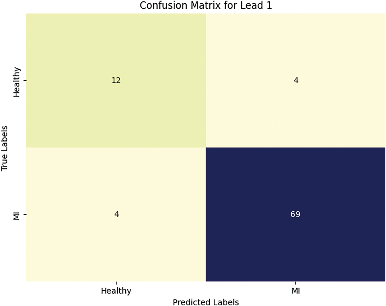
Figure 10: The number of true and false predictions for lead I

The trends observed from the confusion matrix in Fig. 10 are as follows: four healthy patients were falsely labeled by the neural networks as having MI. Meanwhile, all cases of myocardial infarction were correctly classified, which confirms the model’s high accuracy and completeness for myocardial infarction.

We also conducted studies in which multiple neural network training was conducted under various parameters, in order to determine the quality indicators of neural network training. After each procedure, the following training parameters were calculated: specificity, sensitivity, training error, and training time. The neural network training results are presented in Tables 8 and 9.

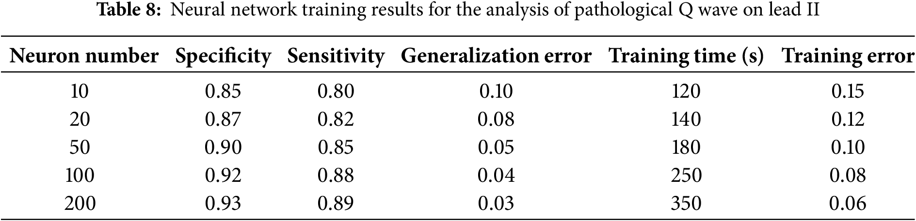
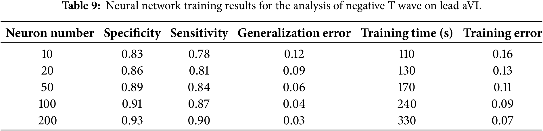
The analyses presented in Tables 8 and 9 highlight the average values of specificity and sensitivity, at the levels of 85% and 90%, respectively. These results demonstrate the high accuracy of the model in identifying both positive and negative cases, which confirms the model’s efficiency in diagnosing pathological changes from ECG data.

4  Discussion

This study demonstrated the successful implementation of machine learning algorithms—in particular, learning vector quantization (LVQ)—for the diagnosis of myocardial infarction based on the data obtained from 12-lead electrocardiograms. The classification accuracy of 87% achieved by the proposed model confirms its high efficiency for the automated diagnosis of cardiovascular diseases. These results underscore the significance of utilizing multi-channel data to enhance the accuracy of myocardial damage localization—a critical component of clinical strategies. One of our key research findings relates to the importance of using 12-channel ECG for enhanced diagnostic accuracy. The inclusion of all 12 leads allowed us to obtain high values in all metrics, including precision, recall, and F1 scores, especially for patients with myocardial infarction, where the F1 score was 92%. The advantage of using a multi-channel system is its ability to more precisely identify damaged areas of the heart, which was confirmed through the analysis of 445 ECG recordings, including 79 from healthy subjects and 366 from patients with myocardial infarction.Pre-processing the data also played a significant role in enhancing the quality of the analysis. The normalization, noise filtering, and scaling of signal amplitudes at a sampling frequency of 1000 Hz and 16-bit resolution enabled the minimization of artifacts and improved the recognition of core elements of ECG signals, such as PQRST waves. The model’s final metrics were positively impacted by the more precise and consistent results obtained during the data processing stage.Despite these promising results, the adaptation of the model for portable devices with a four-channel ECG system remains a challenge due to the potential loss of diagnostic precision. However, the computational efficiency of the proposed LVQ model makes it highly suitable for real-time diagnostics in wearable devices. This allows healthcare professionals to continuously monitor patient data remotely and provides patients with a convenient tool for self-monitoring, reducing the risk of complications through timely diagnostics. Future research will aim to adapt and evaluate the proposed method for four-channel ECG systems to ensure effective real-time diagnostics with fewer input channels.

5  Conclusions

This study confirmed the efficiency of using the LVQ algorithm for the diagnosis of myocardial infarction utilizing a 12-lead ECG system, presenting an overall accuracy of 87%. The main advantage was the capability for accurate localization of myocardial damage via multi-channel analysis. Data pre-processing proved to be a crucial step for improving signal quality and enhancing the accuracy of the trained model. Further plans involve adapting this method for implementation in wearable devices utilizing a four-channel system, thereby expanding the potential applications of the proposed technology in daily life. The obtained results validate the efficacy of machine learning methods in the field of cardiologic diagnostics and establish a basis for potential improvements in this domain.

The proposed LVQ model demonstrates high diagnostic accuracy alongside low classification time, making it a suitable candidate for integration into wearable devices for real-time myocardial infarction detection. This approach facilitates continuous cardiac monitoring outside of clinical settings, enabling timely and accurate diagnostic feedback for healthcare providers while offering patients a convenient and effective tool for self-monitoring. Such advancements have the potential to enhance patient outcomes and reduce the risk of complications through more efficient health management.

Acknowledgement: The authors would like to express their sincere gratitude to Kairat Karibayev, Head of the Cardiology Center at the Central Clinical Hospital of Almaty, for his invaluable support and expert guidance throughout the course of this research.

Funding Statement: This research was funded by the Ministry of Science and Higher Education of the Republic of Kazakhstan, grant numbers AP14969403 and AP23485820.

Author Contributions: Conceptualization, Zhadyra Alimbayeva and Kassymbek Ozhikenov; Data curation, Aiman Ozhikenova; Funding acquisition, Zhadyra Alimbayeva; Investigation, Yeldos Altay; Methodology, Chingiz Alimbayev; Project administration, Zhadyra Alimbayeva; Resources, Yeldos Altay and Aiman Ozhikenova; Software, Zhadyra Alimbayeva; Supervision, Kassymbek Ozhikenov; Validation, Zhadyra Alimbayeva; Visualization, Zhadyra Alimbayeva; Writing—original draft, Zhadyra Alimbayeva; Writing—review and editing, Chingiz Alimbayev. All authors reviewed the results and approved the final version of the manuscript.

Availability of Data and Materials: https://gist.github.com/zhadyralimbay/7445957b9483277d850d5ebe4d1a2c24#file-31-08-ipynb-ipynb (code for analyzing medical data using neural networks to predict myocardial infarction) (assessed 10 January 2025).

Ethics Approval: This study was conducted using publicly available ECG data sets obtained from the PTB Diagnostic ECG Database, hosted on PhysioNet. The data were collected in accordance with ethical guidelines, anonymized, and made freely accessible for research purposes. Therefore, the study did not require additional ethical approval. The use of this database complies with the Open Data Commons Attribution License.

Conflicts of Interest: The authors declare no conflicts of interest to report regarding the present study.

References

1. Gaidai O, Cao Y, Loginov S. Global cardiovascular diseases death rate prediction. Curr Probl Cardiol. 2023;48(5):101622. doi:10.1016/j.cpcardiol.2023.101622. [Google Scholar] [PubMed] [CrossRef]

2. Gong FF, Vaitenas I, Malaisrie SC, Maganti K. Mechanical complications of acute myocardial infarction: a review. JAMA Cardiol. 2021;6(3):341–9. doi:10.1001/jamacardio.2020.3690. [Google Scholar] [PubMed] [CrossRef]

3. Kayikcioglu İ, Akdeniz F, Köse C, Kayikcioglu T. Time-frequency approach to ECG classification of myocardial infarction. Comput Electr Eng. 2020;84:106621. doi:10.1016/j.compeleceng.2020.106621. [Google Scholar] [CrossRef]

4. Aslanger E, Yıldırımtürk Ö, Şimşek B, Sungur A, Türer Cabbar A, Bozbeyoğlu E, et al. A new electrocardiographic pattern indicating inferior myocardial infarction. J Electrocardiol. 2020;61:41–6. doi:10.1016/j.jelectrocard.2020.04.008. [Google Scholar] [PubMed] [CrossRef]

5. Sridhar C, Lih OS, Jahmunah V, Koh JEW, Ciaccio EJ, San TR, et al. Accurate detection of myocardial infarction using non linear features with ECG signals. J Ambient Intell Humaniz Comput. 2021;12(3):3227–44. doi:10.1007/s12652-020-02536-4. [Google Scholar] [CrossRef]

6. Corya BC, Rasmussen S, Knoebel SB, Feigenbaum H. Echocardiography in acute myocardial infarction. Am J Cardiol. 1975;36(1):0002914975908590. doi:10.1016/0002-9149(75)90859-0. [Google Scholar] [PubMed] [CrossRef]

7. Degerli A, Kiranyaz S, Hamid T, Mazhar R, Gabbouj M. Early myocardial infarction detection over multi-view echocardiography. Biomed Signal Process Contr. 2024;87:105448. doi:10.1016/j.bspc.2023.105448. [Google Scholar] [CrossRef]

8. Si N, Shi K, Li N, Dong X, Zhu C, Guo Y, et al. Identification of patients with acute myocardial infarction based on coronary CT angiography: the value of pericoronary adipose tissue radiomics. Eur Radiol. 2022;32(10):6868–77. doi:10.1007/s00330-022-08812-5. [Google Scholar] [PubMed] [CrossRef]

9. Chaulin AM, Duplyakov DV. Biomarkers of acute myocardial infarction: diagnostic and prognostic value. Part 1. J Clin Pract. 2020;11(3):75–84. doi:10.17816/clinpract34284. [Google Scholar] [CrossRef]

10. Tilea I, Varga A, Serban RC. Past, present, and future of blood biomarkers for the diagnosis of acute myocardial infarction-promises and challenges. Diagnostics. 2021;11(5):881. doi:10.3390/diagnostics11050881. [Google Scholar] [PubMed] [CrossRef]

11. Al-Zaiti S, Martin-Gill C, Zègre-Hemsey J, Bouzid Z, Faramand Z, Alrawashdeh MO, et al. Machine learning for ECG diagnosis and risk stratification of occlusion myocardial infarction. Nat Med. 2022;29:1804–13. doi:10.1038/s41591-023-02396-3. [Google Scholar] [PubMed] [CrossRef]

12. Ibrahim L, Mesinovic M, Yang KW, Eid MA. Explainable prediction of acute myocardial infarction using machine learning and shapley values. IEEE Access. 2020;8:210410–7. doi:10.1109/ACCESS.2020.3040166. [Google Scholar] [CrossRef]

13. Xiong P, Lee SM, Chan G. Deep learning for detecting and locating myocardial infarction by electrocardiogram: a literature review. Front Cardiovasc Med. 2022;9:860032. doi:10.3389/fcvm.2022.860032. [Google Scholar] [PubMed] [CrossRef]

14. Hasbullah S, Mohd Zahid MS, Mandala S. Detection of myocardial infarction using hybrid models of convolutional neural network and recurrent neural network. BioMedInformatics. 2023;3(2):478–92. doi:10.3390/biomedinformatics3020033. [Google Scholar] [CrossRef]

15. Alimbayeva Z, Alimbayev C, Ozhikenov K, Bayanbay N, Ozhikenova A. Wearable ECG device and machine learning for heart monitoring. Sensors. 2024;24(13):4201. doi:10.3390/s24134201. [Google Scholar] [PubMed] [CrossRef]

16. Sun Z, Wang C, Zhao Y, Yan C. Multi-label ECG signal classification based on ensemble classifier. IEEE Access. 2020;8:117986–96. doi:10.1109/ACCESS.2020.3004908. [Google Scholar] [CrossRef]

17. Pan W, An Y, Guan Y, Wang J. MCA-net: a multi-task channel attention network for Myocardial infarction detection and location using 12-lead ECGs. Comput Biol Med. 2022;150:106199. doi:10.1016/j.compbiomed.2022.106199. [Google Scholar] [PubMed] [CrossRef]

18. Sahu G, Ray KC. An efficient method for detection and localization of myocardial infarction. IEEE Trans Instrum Meas. 2021;71:4001312. doi:10.1109/TIM.2021.3132833. [Google Scholar] [CrossRef]

19. Zhang J, Liu M, Xiong P, Du H, Zhang H, Lin F, et al. A multi-dimensional association information analysis approach to automated detection and localization of myocardial infarction. Eng Appl Artif Intell. 2021;97:104092. doi:10.1016/j.engappai.2020.104092. [Google Scholar] [CrossRef]

20. Alimbayeva ZN, Alimbayev CA, Bayanbay NA, Ozhikenov KA, Bodin ON, Mukazhanov YB. Portable ECG monitoring system. Int J Adv Comput Sci Appl. 2022;13(4):64–76. doi:10.14569/IJACSA.2022.0130408. [Google Scholar] [CrossRef]

21. Liao Y, Tang Z, Gao K, Trik M. Optimization of resources in intelligent electronic health systems based on Internet of Things to predict heart diseases via artificial neural network. Heliyon. 2024;10(11):e32090. doi:10.1016/j.heliyon.2024.e32090. [Google Scholar] [PubMed] [CrossRef]

22. Gustafsson S, Gedon D, Lampa E, Ribeiro AH, Holzmann MJ, Schön TB, et al. Development and validation of deep learning ECG-based prediction of myocardial infarction in emergency department patients. Sci Rep. 2022;12:19615. doi:10.1038/s41598-022-24254-x. [Google Scholar] [PubMed] [CrossRef]

23. Jahmunah V, Ng EYK, Tan RS, Oh SL, Acharya UR. Explainable detection of myocardial infarction using deep learning models with Grad-CAM technique on ECG signals. Comput Biol Med. 2022;146:105550. doi:10.1016/j.compbiomed.2022.105550. [Google Scholar] [PubMed] [CrossRef]

24. Goldberger AL, Amaral LA, Glass L, Hausdorff JM, Ivanov PC, Mark RG, et al. Physiobank, physiotoolkit, and physionet: components of a new research resource for complex physiologic signals. Circulation. 2000;101(23):e215–20. doi:10.1161/01.cir.101.23.e215. [Google Scholar] [PubMed] [CrossRef]