
 Submit a Paper
 Propose a Special lssue
 Open Access
ARTICLE
Hybrid Memory-Enhanced Autoencoder with Adversarial Training for Anomaly Detection in Virtual Power Plants
1 Department of Computer Engineering, Chonnam National University, Yeosu, 59626, Republic of Korea
2 Department of Cultural Contents, Chonnam National University, Yeosu, 59626, Republic of Korea
* Corresponding Authors: YeonJae Oh. Email: ; Chang Gyoon Lim. Email:
Computers, Materials & Continua 2025, 82(3), 4593-4629. https://doi.org/10.32604/cmc.2025.061196
Received 19 November 2024; Accepted 15 January 2025; Issue published 06 March 2025
 View Full Text
 Download PDF
Abstract
Virtual Power Plants (VPPs) are integral to modern energy systems, providing stability and reliability in the face of the inherent complexities and fluctuations of solar power data. Traditional anomaly detection methodologies often need to adequately handle these fluctuations from solar radiation and ambient temperature variations. We introduce the Memory-Enhanced Autoencoder with Adversarial Training (MemAAE) model to overcome these limitations, designed explicitly for robust anomaly detection in VPP environments. The MemAAE model integrates three principal components: an LSTM-based autoencoder that effectively captures temporal dynamics to distinguish between normal and anomalous behaviors, an adversarial training module that enhances system resilience across diverse operational scenarios, and a prediction module that aids the autoencoder during the reconstruction process, thereby facilitating precise anomaly identification. Furthermore, MemAAE features a memory mechanism that stores critical pattern information, mitigating overfitting, alongside a dynamic threshold adjustment mechanism that adapts detection thresholds in response to evolving operational conditions. Our empirical evaluation of the MemAAE model using real-world solar power data shows that the model outperforms other comparative models on both datasets. On the Sopan-Finder dataset, MemAAE has an accuracy of 99.17% and an F1-score of 95.79%, while on the Sunalab Faro PV 2017 dataset, it has an accuracy of 97.67% and an F1-score of 93.27%. Significant performance advantages have been achieved on both datasets. These results show that MemAAE model is an effective method for real-time anomaly detection in virtual power plants (VPPs), which can enhance robustness and adaptability to inherent variables in solar power generation.Keywords
Virtual Power Plants (VPPs) are an essential development in power system management. They offer flexible solutions to challenges such as connecting renewable energy to the grid, keeping the grid stable, and managing energy demand on the consumer side [1]. Initially, the main idea behind VPPs was to combine small-scale distributed energy resources (DERs) into one system [2]. Over time, technological movements have made VPPs more advanced tools. They can now manage a broader range of energy resources, such as solar panels, wind turbines, energy storage systems, and demand response units [3]. This progress has made VPPs a necessary part of modern energy systems. They are essential for balancing energy supply and demand while also helping to promote sustainable development.
Although the concept of VPPs was first proposed in the 1990s, it only began to gain momentum in the early 2000s with the widespread adoption of distributed energy resources. In the early days, virtual power plants mainly focused on coordinating and optimizing the integration of distributed energy resources to improve operational efficiency and the power grid’s reliability. However, due to technological limitations, incomplete policies and regulations, and the initial development stage of distributed power generation technology, the actual deployment of VPPs was still mainly at the theoretical level at that time.
The primary function of Virtual Power Plants (VPPs) is to help integrate renewable energy smoothly into the grid. They achieve this by bringing together distributed energy resources and improving grid control to make grid management more efficient [4]. VPPs combine different energy sources, such as solar power, wind power, energy storage systems, and controllable loads, into one system. As a unified entity, VPPs can participate in electricity markets and support grid operations by providing energy and additional services. This approach increases the flexibility of the power grid and helps improve energy efficiency. At the same time, it lowers carbon emissions, making VPPs an essential part of the movement toward a more sustainable energy future.
In recent years, the development of virtual power plants (VPPs) has been mainly driven by multiple essential factors, including the widespread adoption of distributed generation technologies such as solar photovoltaics and wind energy, the reduction of communication and control system costs, and the increasing desire of consumers (both producers and consumers) to participate in the energy market and achieve self-sufficiency [5]. These trends make VPPs more economically feasible and technologically mature.
1.1 Supervisory Control and Data Acquisition (SCADA) System
Earlier, we discussed the different parts that make up virtual power plants. Information and Communication Technology (ICT), especially SCADA systems, makes VPPs work effectively by enabling efficient monitoring and control of distributed energy resources. SCADA systems provide advanced solutions for remote monitoring, control, and optimization of different processes, making them essential in managing the complexities of VPPs.
SCADA systems were initially designed to manage local industrial processes. Still, as technology has advanced, they have evolved into powerful tools capable of overseeing complex machinery and sensor networks spread across large geographic areas [6]. Today, SCADA systems are widely used in energy production, manufacturing, water treatment, and transportation to ensure efficient and reliable operations [7].
The concept of SCADA originated in the mid-20th century when industrial organizations sought more efficient solutions for remote equipment control. In the 1960s, telemetry technology enabled automated communication between remote sites and central control stations, laying the foundation for developing early SCADA systems. These systems would allow operators to manage industrial processes without physically visiting each site, a revolutionary advancement in industrial automation [8]. A typical SCADA system architecture, as depicted in Fig. 1, showcases the significant components of a SCADA system and how they interact:

Figure 1: SCADA system structure
Fig. 1 shows the overall architecture of a SCADA system, including historical databases, communication links, MTUs, RTUs, human-machine interfaces (HMI), operators, data analysis modules, and communication between field devices.
Historian stores all real-time data collected from field devices and RTUs [9]. The stored data can be used for subsequent analysis to optimize equipment operation, improve system efficiency, and provide decision support. Historical databases’ long-term data storage capabilities provide complete data records for SCADA systems. Communication Link connects the central terminal unit, the remote terminal unit, and the HMI to achieve real-time data transmission [10]. Different wired or wireless methods, such as LAN, WAN, optical fiber, radio, etc., can serve as communication links. It is the data transmission channel of the entire SCADA system, ensuring reliable data communication between individual modules.
The MTU is the core control unit of the SCADA system [11]. It is responsible for receiving, processing, and storing data from the RTU and sending commands to the RTU based on pre-set control logic to control the operation of the field equipment. The MTU is connected to the HMI to provide the operator with real-time system status and alarm information.
RTU acts as a bridge between SCADA systems and field devices, collecting real-time data from field devices such as sensors and actuators and sending it to MTU. It can also receive control instructions from the MTU to adjust the device’s operating status. In addition to RTUs, programmable logic controllers (PLCs) and intelligent electronic devices (IEDs) are mentioned in the figure, which can be used in more complex control scenarios to achieve multifaceted control.
This communication section between field devices and RTU/IEDs/PLC represents the data exchange between field devices (sensors and actuators) and RTUs, IEDs, or PLCs. Through these devices, the SCADA system can obtain field information in real-time and perform control operations to ensure the system’s regular operation.
HMI provides the operator with a visual interface through which the operator can monitor the status of the field equipment in real-time, view system alarms, view historical data, and manually control the system. HMI is connected to the MTU to monitor and manage the SCADA system. The operator interacts with the SCADA system via HMI, monitors the system’s operation status, analyzes the data, and takes appropriate measures as needed.
The operator plays a vital role in the SCADA system and is responsible for the timely handling of alarm information and performing system control. Data analytics is in the intranet of SCADA systems and is used to analyze historical data to help optimize system performance and improve productivity.
Data analysis can identify anomalies in operation, generate trend analysis and reports, and provide data support for system maintenance and decision-making. Distributed around the company, the Field Device includes a collection of tools used to track and manage production operations. Many sensors gather information, while actuators carry out control functions. Specialized communication protocols have been developed to ensure uninterrupted, dependable, and effective communication among SCADA components.
As additional renewable energy sources, such as solar, are integrated into the power grid, ensuring these systems operate consistently and efficiently is critical. This requires real-time monitoring, rapid anomaly detection, quick problem resolution, and ensuring peak system performance.
Certain technologies, such as autoencoders, are effective in handling time-series data, especially data produced by power systems. With the increasing integration of renewable energy sources, real-time monitoring and advanced anomaly detection have become essential to maintaining stability and efficiency. However, working with solar data can introduce specific challenges. Solar data is often complex and variable due to environmental factors, making certain minor anomalies challenging to detect. This places higher demands on autoencoders.
With the rapid development of industrial automation and control technologies, SCADA systems face increasingly complex challenges when processing time series data. Traditional anomaly detection methods, such as reconstruction-based autoencoders, sometimes work well. Still, their effectiveness could be improved when dealing with more complex data patterns, such as contextual or collective anomalies. Fig. 2 shows the point anomalies captured by the autoencoder.

Figure 2: Point anomalies captured by autoencoders
It uses traditional reconstruction-based methods for anomaly detection. The red line represents an anomaly, and the blue line represents a reconstruction. Based on previous studies, anomalies can be categorized into different types, such as point exceptions, contextual anomalies, and collective exceptions. Reconstruction-based models are generally better at detecting point anomalies because they depend on point-by-point reconstruction errors (refer to Fig. 3). However, detecting contextual and collective exceptions is more challenging.

Figure 3: Contextual anomalies ignored by autoencoders
As shown in Fig. 3, the black line represents average data, the blue line represents reconstructed data, and the red line represents abnormal data. These anomalies only deviate from the usual pattern in certain situations, and their numerical values remain close to normal.
The strong generalization capabilities of neural networks enable autoencoders to reconstruct data with remarkably high accuracy, even in exceptional cases. This is due to overfitting, structural similarities between normal and abnormal data, and the absence of clear boundaries between the two. In addition, when abnormal data isn’t adequately labeled during training, autoencoders tend to make reconstruction errors less noticeable at these abnormal data points, which makes the issue worse. New models integrating modern technologies, such as generative adversarial networks (GANs) [12], have become a necessary solution to overcome these limitations.
So, we can see that traditional refactoring-based self-encoders face many challenges in exception detection, especially when dealing with context and collective exceptions. Point anomalies are easier to detect because individual data points deviate significantly from standard patterns [13]. However, contextual anomalies depend on the time series; single-point values may be typical but overall pattern anomalies, while collective anomalies are reflected in the pattern deviations of a set of data [14]. In addition, there is often abnormal pollution in actual data; that is, unlabeled abnormal data is mistaken for standard data, which causes the model reconstruction error to shrink, masking the actual abnormalities and reducing the detection effect [15]. At the same time, external factors, such as light, temperature, wind speed, etc., in dynamic environments (such as photovoltaic systems) make the data pattern constantly changing, and traditional fixed thresholds cannot adapt to these real-time dynamic changes [16]. In addition, the generalization and robustness of the model are also outstanding. Traditional methods easily overfit standard data are sensitive to noise data and lack effective memory mechanisms to store and distinguish normal and abnormal patterns [17].
To address these limitations, this study introduces a Memory-Enhanced Autoencoder with Adversarial Training (MemAAE) framework [18]. The memory module enables the model to store and distinguish between normal and abnormal patterns over long-time dependencies, effectively capturing contextual and collective anomalies [19]. Furthermore, adversarial training strengthens the model’s robustness against noisy data, mitigating the impact of abnormal contamination and improving generalization. This framework not only overcomes the shortcomings of traditional autoencoders but also adapts to dynamic environmental changes, providing a robust solution for real-time anomaly detection in complex time-series data.
The time series anomaly detection field has attracted much attention in recent years [20–23]. Traditional anomaly detection methods define anomalies as significantly different values from most data points, which can be divided into several categories, including distance-based methods [24], density estimation techniques, isolation-based methods, and statistical inference-driven methods [21,22].
2.1 Prediction-Based Time-Series Anomaly Detection
With the rapid advancement of deep learning technology, the time series anomaly detection field has entered a new era filled with opportunities and challenges. The latest research literature, including studies like “Deep Learning Time Series Anomaly Detection Investigation” and “Deep Learning Time Series Data Anomaly Detection Review and Analysis” [24], offers a broad overview of deep learning applications in this area.
These papers explore both the strengths and limitations of various anomaly detection techniques. They also provide examples of deep anomaly detection in several application fields, showcasing developments from recent years.
In addition, ALAD’s unsupervised time-series anomaly detection paradigm based on activation learning provides a new method for anomaly detection [25]. Deep learning models are very good at automating tasks and being accurate. They can handle multidimensional time series data and pick up on long-term dependencies. However, they need a lot of training data and computing power, and the models are more complex to understand, which can be a problem in some situations.
2.2 Reconstruction-Based Time-Series Anomaly Detection
Recently, a new method based on the reconstruction of time series anomaly detection has been proposed, focusing on improving the model’s robustness and accuracy. Geometric distribution masks are used to make the training data more varied, and transformer-based autoencoders are trained in the GAN framework to solve the overfitting problem [26].
In addition, introducing contrast loss to the discriminator helps regulate the GAN and improve the generalization capability [12]. The experimental results show that the method significantly improves the accuracy, reproducibility, and F1-score of the real-world dataset.
The ConvBiLSTM-AE model serves as a reference for encoder selection due to its ability to handle multivariate time series data in industrial control systems [27]. By combining the spatial feature extraction capabilities of Convolutional Neural Networks RE(CNNs) Mean Squared Error (MSE) with the temporal dependencies captured by Bidirectional Long Short-Term Memory (BiLSTM) networks, it effectively addresses the complexities of industrial data. In contrast, the MemAAE model incorporates an LSTM-based self-encoder, a memory module, adversarial training, and a prediction module to enhance anomaly detection robustness in virtual power plant environments. This model improves detection performance by memorizing key patterns and dynamically adjusting thresholds to adapt to environmental changes. While ConvBiLSTM-AE excels at processing complex industrial data, the MemAAE model offers greater complexity and adaptability through its innovative memory and adversarial training mechanisms, making it particularly effective in environments where dynamic thresholds and memory-driven insights are essential for accurate anomaly detection.
Memory has played a crucial role in developing anomaly detection systems within deep learning. LSTM and GRU architecture employ memory cells to retain information about past states, as evidenced by their reliance on historical data in contrastive learning methods. In time series anomaly detection, memory-based approaches have been utilized to mitigate the misapplication of anomaly data across datasets [28]. However, these methods are not explicitly tailored for time series data and do not fully address the critical challenges inherent in time series anomaly detection.
2.4 Innovations and Contributions
Most current methods use fixed thresholds to judge anomalies, making it difficult to adapt to complex dynamic environments, such as severe fluctuations in environmental variables such as light and temperature [29]. This static threshold design can easily lead to the model’s omission or misdetection in non-stationary time series data. In addition, reconstruction error and prediction error methods are fragile in the face of noise data, and the generalization ability is weak, which affects the practical application effect [30]. Traditional time-dependent modeling methods, such as LSTM and GRU, have a specific memory capacity but lack a clear distinction between normal and abnormal patterns, making it challenging to identify complex abnormal events accurately.
In view of these challenges, an innovative time-series anomaly detection framework combining dynamic thresholds, self-encoders, and memory modules is proposed. Through the introduction of a dynamic threshold mechanism, the model can adjust the anomaly detection standard according to real-time input data to effectively adapt to dynamic environmental changes, especially in photovoltaic systems. At the same time, this study designed a memory module to store the key features of normal and abnormal patterns, enhancing the modeling ability of time-dependent relationships and improving the detection effect of complex time-series anomalies [31]. To further improve the robustness and generalization of the model, this paper introduces a generative adversarial training mechanism, which effectively suppresses the influence of noise data through adversarial learning between the generator and the discriminator [12].
The preprocessing steps of the dataset in this paper are shown in Fig. 4.

Figure 4: Data preprocessing workflow for handling missing values and feature engineering
The data preprocessing process consists of the following steps: First, check the source of missing values in the dataset, analyze the proportion of missing values in each column, delete the column if the missing value exceeds 50%, and smooth and fill in the missing value. The timestamp data is then processed to extract time features such as year, month, day, hour, and minute to generate a new column. Subsequently, correlations between features are calculated, and columns with correlation coefficients greater than 0.2 are retained to remove low-correlation features. Normalize or standardize reserved features to ensure that data distribution is appropriate for model inputs. Methods such as linear interpolation are used to fill out the remaining missing values, while time series data are resampled to ensure that the data intervals are uniform. After the above steps, complete the data preprocessing to provide high-quality input for subsequent modeling.
The data set used in this research paper comes from the Sopan-Finder repository. This repository is a source for collecting and analyzing data about solar power systems. This data is collected through the SCADA system, which stands for Supervisory Control and Data Acquisition, as cited in reference. The dataset includes a variety of time-series features. These features include data on environmental conditions and system performance indicators. Together, they form a resource that helps detect anomalies in solar power generation. Because this dataset is directly from solar energy systems, it gives important insights for this study.
The dataset covers about 7703.75 h of data, close to 320 days of important environmental and operational information. It contains a total of 30,816 separate data points. Each data point has a specific timestamp that marks the exact time of each measurement. Abnormal system behavior is identified based on power output, as represented by PV_Demand. When the PV_Demand goes below a threshold of 0.1, it is marked as an anomaly. However, it is important to note that these anomalies do not originate from Virtual Power Plant (VPP) operational scenarios but rather stem from solar panel shutdowns or faults.
In this dataset, 15.93% of data points are considered anomalies, highlighting the significance of these events. Table 1 includes a summary of key indicators for easy reference.

The dataset’s time features include each record’s month, day, hour, and minute. This level of granularity provides a detailed timestamp for every observation. Such detail enables accurate time-series analysis, helping researchers identify patterns, trends, and seasonal changes in the data, especially for critical variables like temperature and PV_Demand.
Weather events such as rain, snow, and precipitation are recorded hourly as rain_1h, snow_1h, and precipitation_1h. Each has 7703 records, which suggests that these measurements are either taken less frequently or only under specific conditions, like when precipitation is detected. These factors can help identify anomalies in power generation, as they often cause a drop in solar energy production.
The PV_Demand variable contains 30,816 records. Each record represents an important indicator of PV_Demand within the data collection period. Examining PV_Demand alongside weather data, such as temperature, wind speed, and cloud cover, provides valuable insights. These insights reveal how environmental factors affect power generation and PV_Demand. Factors like temperature, cloud cover, and rainfall are important in modeling solar power. They directly influence sunlight availability and the efficiency of solar panels. With data over 7700 h, this dataset forms a strong basis for analyzing long-term trends. It also helps recognize seasonal patterns and identify anomalies that arise due to environmental or operational changes.
This paper also visualizes the anomaly data. PV_Demand and temperature are visualized because they are important factors in finding anomalies (the highest correlation coefficients with labels are 0.4198 for PV_Demand and 0.5724 for temperature). Fig. 5 shows how these two factors were used to visualize the anomalies.

Figure 5: Exception data visualization
The visualization results of the anomaly points are presented below. The horizontal axis represents the photovoltaic system’s power output (PV_Demand, in kW), while the vertical axis represents the temperature (in Celsius). Each point on the graph corresponds to a specific sample from the dataset, with green dots representing standard data and red dots representing anomalies. Many anomalies are concentrated on the far left of the graph, where PV_Demand is close to or equal to zero, suggesting system shutdowns or failures during these periods. These anomalies primarily occur across a temperature range of approximately −10°C to 35°C, most concentrated at medium-to-low temperatures. As PV_Demand increases beyond 20 kW, anomalies become much less frequent, highlighting that the photovoltaic system performs reliably under higher power generation conditions. This pattern indicates a strong relationship between anomalies, low PV_Demand, and temperature variations, with anomalies predominantly arising during low-temperature periods and inactive or shutdown states of the photovoltaic system.
2.5.3 Sunlab Faro PV 2017 Dataset
To further validate our proposed model’s generalization ability, we used the SunLab Faro PV 2017 dataset obtained from EDP SunLab. This dataset primarily monitors the operational status and performance of two solar panels, Panel A and Panel B. The dataset includes key time-series features such as voltage, current, and power output for each panel under vertical, optimal tilt, and horizontal orientations. Additionally, it contains temperature measurements for the panels’ surfaces in each orientation, reflecting their thermal conditions during operation. The dataset also includes high-resolution timestamps with year, month, day, hour, and minute, allowing detailed time-series analysis.
The dataset includes key time-series features such as voltage, current, and power output for each panel under vertical, optimal tilt, and horizontal orientations. Additionally, it contains temperature measurements for the panels’ surfaces in each orientation, reflecting their thermal conditions during operation. The dataset also includes high-resolution timestamps with year, month, day, hour, and minute, allowing detailed time-series analysis. The specific features are shown in Table 2.

The dataset contains 100,000 data points, corresponding to a time span of approximately 1666.67 h. Table 2 summarizes the dataset’s specific features. Fig. 6 demonstrates the relationship between temperature, power output, and anomalies for different panels and orientations.
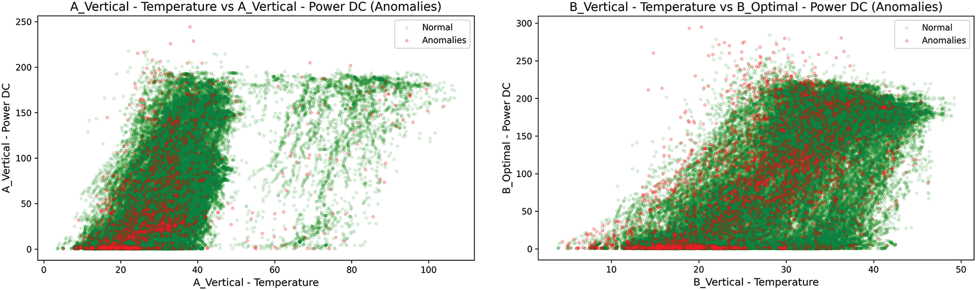
Figure 6: Anomaly visualization
The anomalies observed in the dataset, as shown in Fig. 6 and summarized in Table 2, are primarily concentrated at low power outputs across all temperature ranges and panel orientations. This suggests that the anomalies are primarily caused by system faults or shutdowns rather than environmental conditions alone. While temperature variations influence the overall power generation, clustering anomalies near zero power output indicate periods of panel inactivity or operational failures.
3 Process Framework and Model Introduction
To enhance the SCADA (Supervisory et al.) system’s capability for real-time monitoring and anomaly detection in solar power systems, we integrated the MemAAE anomaly detection model. The model takes data from the SCADA system, such as solar irradiance, temperature, and power output, and calculates reconstruction and prediction errors. When errors exceed dynamically set thresholds, the SCADA system marks the data as abnormal and alerts the operator in real time, enabling prompt investigation and corrective action. This mechanism ensures rapid intervention and prevents potential failures in solar power systems.
Fig. 7 shows the MemAAE model, an anomaly detection process based on the LSTM self-encoder. This model is mainly used for data monitoring and anomaly detection in solar power systems.

Figure 7: Memory-augmented adversarial autoencoder for anomaly detection
First, the SCADA architecture collects the data, including sensors, PLC/RTUs, and server infrastructure, which are cleaned and normalized during the data preprocessing phase. The preprocessed data is fed into the MemAAE model, where the core consists of an LSTM self-encoder. The model consists of an input layer, a hidden layer, and an output layer, and the LSTM network is responsible for learning the time-dependent patterns of the data and reconstructing the input data.
Memory modules are introduced into the network to store and retrieve critical standard data patterns and enhance the model’s ability to recognize abnormal data. In addition, the model includes a prediction branch that generates predictions for future steps to assist in reconstruction tasks and improve the effectiveness of anomaly detection.
The model judges the authenticity of the data by combining reconstruction error with prediction error. The output module classifies the anomalies by dynamic threshold detection mechanism, and the results are divided into standard (blue) and outlier (red). The framework utilizes MemAAE’s memory mechanism and LSTM’s time modeling capabilities to accurately capture anomaly data and improve the system’s anomaly detection performance in complex time series environments.
3.1 Time-Series Data Preprocessing
Larger values in the vibration data expand its scale. This makes the model insensitive to subtle changes in smaller values and may cause it to overlook important features. We need to address this issue and consider sensor context data simultaneously. Therefore, raw data for all time dimensions must be standardized. Standardization ensures that all features are within the same scale range, preventing features with larger values from disproportionately affecting the model. It also helps to capture small but critical changes. This process speeds up the model’s convergence and improves numerical stability [32].
The raw data D ∈
where X is the raw data matrix, µ is the mean of each feature, calculated as:
where σ is the standard deviation of each feature, calculated as:
Standardization transforms the data into a mean of 0 and a standard deviation of 1, ensuring that different features are processed on the same scale.
Next, the sliding window technique is applied to the standardized data to segment it, enabling the capture of temporal dependencies in the time series. The sliding window divides the data into multiple fixed-length windows, each containing a series of time steps. The sliding window operation can be represented by:
where
3.2 Autoencoder (Encoder-Decoder)
The encoder encodes the input data using two LSTM layers. The main reason for choosing an LSTM self-encoder over a GRU is that LSTM is better suited to handle long-term dependencies, has better memory capabilities, and has higher modeling accuracy. LSTM’s three-door structure (input gate, forget gate, output gate) allows it to control the flow of information more finely, especially for complex time series reconstruction and anomaly detection tasks. While GRU calculations are more efficient, LSTM performance is more stable and reliable when dealing with tasks requiring long sequences and high precision. Fig. 8 illustrates the architecture of a single LSTM network.
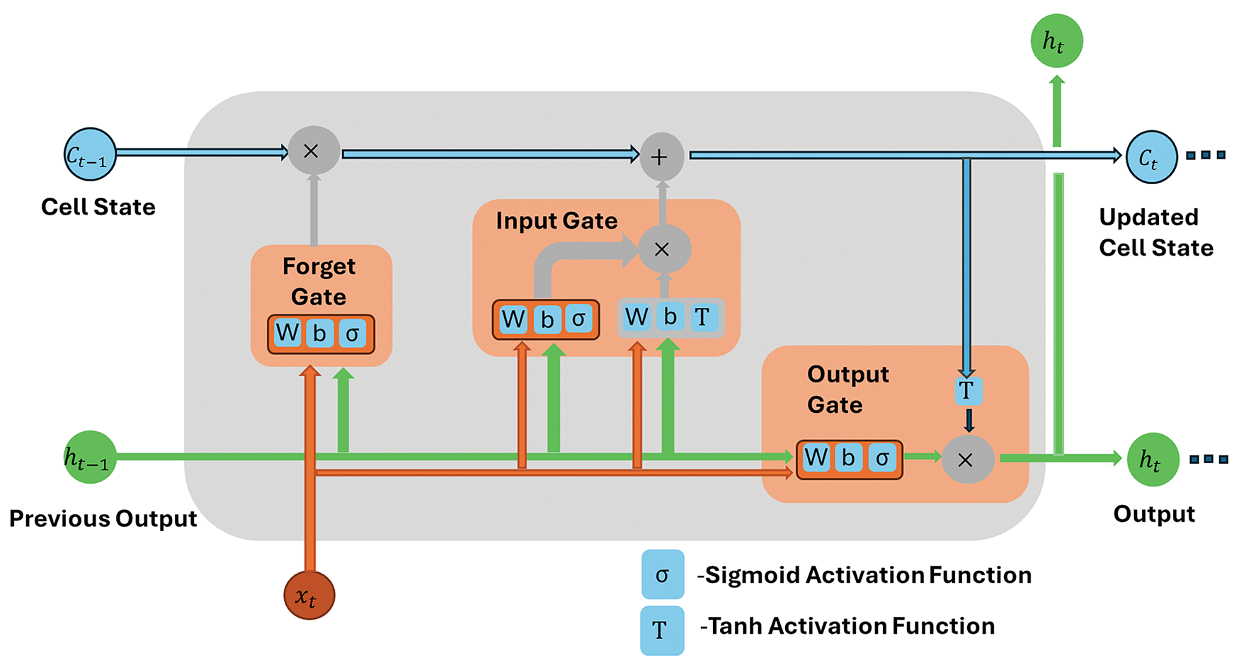
Figure 8: The architecture of a LSTM
The forget gate determines how much of the previous cell state
The activation function of the forget gate is the sigmoid function, which guarantees that the output vector from the gate produces continuous values ranging from 1 (retain) to 0 (discard). The subscript ‘
The input gate controls how much new information will be added to the cell state. The corresponding formulas are presented below, labeled as Eqs. (7) to (9):
This gate employs two operational units. The first functional unit employs a
The output gate controls the amount of the cell’s hidden state that is disclosed. These denoted as Eqs. (10) and (11), respectively, describe the output gate:
To retrieve useful information from the input and the preceding output, the output gate employs a trained matrix
The LSTM layers handle sequential data, producing a hidden state
where
The workflow of a typical memory module is shown in Fig. 9.
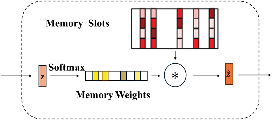
Figure 9: Memory module structure
The memory module consists of a dense layer to compute memory vectors and attention weights using a SoftMax function:
where
The Memory Weights are calculated using a SoftMax function:
The
The SoftMax function ensures that the sum of the weights is 1, which helps focus on the most relevant memory vectors while downweighing less important ones.
The memory output is computed as a weighted sum of the memory vectors:
where
The decoder reconstructs the time series data using the weighted memory output and input:
where
This part of the model reconstructs the original input sequence based on the memory representation. The LSTM layers in the decoder take the memory output and sequentially generate hidden states
3.3 Discriminator (Adversarial Training)
The discriminator distinguishes between real and generated (reconstructed) data points. The discriminator’s output is given by:
where
The discriminator loss function measures how well the discriminator performs in distinguishing between real and fake (generated) data. The loss is split into two parts: one for real data and one for counterfeit data. The following are the formulas for Real Data Loss and the Fake Data Loss, respectively:
where
The negative log-likelihood function is applied to encourage the discriminator to output a value close to 1 for real data. If the discriminator correctly identifies real data,
The total discriminator loss function helps the discriminator learn to differentiate between real and generated data by minimizing the error in both cases:
The total discriminator loss,
3.4 Combined Model (Autoencoder + Discriminator)
The autoencoder and the discriminator are combined and trained adversarial to improve the model’s performance. Eq. (22) for calculating Generator Loss is as shown:
where
The generator adversarial loss evaluates how effectively the autoencoder deceives the discriminator into classifying the generated (reconstructed) data as real. Eq. (23) is as follows:
where
Eq. (24) is the sum of the reconstruction loss and the generator adversarial loss:
The combined loss balances the autoencoder’s two main objectives: minimizing the difference between the original and reconstructed data to ensure the autoencoder can accurately reproduce the input and deceiving the discriminator into thinking that the generated data is real.
The prediction module forecasts future values in the time series based on past observations. It is being shown on Fig. 10.

Figure 10: Prediction module
It utilizes an LSTM (Long Short-Term Memory) layer to predict the next step in the sequence. The prediction output is represented as:
where
The prediction loss measures the accuracy of the model’s forecast by comparing the predicted values
where
The goal is to minimize this loss, encouraging the model to make more accurate predictions over time. By reducing the squared error, the model improves its forecasting capability for future time steps in the sequence.
3.6 Anomaly Detection Criteria
Both reconstruction and prediction errors are used to detect anomalies in the system. The idea is to compare actual data with reconstructed and predicted values, and if these errors exceed certain thresholds, the data points are considered abnormal. This process is shown in Fig. 11.

Figure 11: Sliding window-based anomaly detection process
The reconstruction error measures how well the autoencoder can recreate the input data. It compares the original input
where
The prediction error evaluates how well the model can forecast future values in the time series. It compares the actual future value
where
where
where
In this context, the rationale for selecting the 85th percentile in the dynamic threshold mechanism is to strike a reasonable balance between false positives and false negatives. A higher percentile, such as the 85th, effectively reduces false positives caused by environmental fluctuations or non-anomalous conditions, thereby preventing the system from overreacting. While a higher threshold may increase the risk of false negatives, the 85th percentile typically captures the majority of anomalies and mitigates the risk of overly narrowing the detection range. Furthermore, the dynamic threshold mechanism adapts to real-time environmental data, allowing the system to maintain good flexibility under varying conditions. Therefore, selecting the 85th percentile as the threshold ensures a reduction in false positives while maintaining sufficient sensitivity to detect significant anomalies.
We used accuracy and F1-scores to assess how well the model performs. Accuracy represents the proportion of samples that are correctly classified. It compares this number to the total sample size. This metric gives a straightforward and clear view of how the model performs across the whole dataset. The formula for accuracy is shown in Eq. (31):
where
The total sample count, denoted as
In anomaly detection tasks, where class imbalance is expected, the model must identify anomalies and minimize false positives. Therefore, while accuracy alone may lead to a misleading assessment of model performance, the F1-score provides a more balanced and comprehensive measure of the model’s effectiveness in detecting anomalies. The formula for Precision is given in Eq. (32):
The formula for Recall in Eq. (33):
The formula for F1-score in Eq. (34):
where
4.2 Experiment Environment Settings
The autoencoder is structured with LSTM layers to capture long-term temporal dependencies effectively. The encoder comprises an LSTM layer with 128 units (activation = Rectified Linear Unit (ReLU), return_sequences = True), followed by a Dropout layer (rate = 0.2) for regularization, and a subsequent LSTM layer with 64 units (activation = ReLU, return_sequences = False). To further enhance the model’s ability to memorize critical patterns, a memory module is incorporated, consisting of a Dense layer with 200 Memory Slots (activation = ReLU) and a SoftMax function to compute Memory Weights, which are then combined via a Multiply layer. The decoder’s memory output is repeated across the temporal dimension using a RepeatVector layer with a predefined window size. The reconstruction phase employs an LSTM layer with 64 units (activation = ReLU, return_sequences = True), followed by a Dropout layer (rate = 0.2) and another LSTM layer with 128 units (activation = ReLU, return_sequences = True). The final output is generated through a TimeDistributed Dense layer to match the original input dimensions. The autoencoder is trained using the Adam optimizer (learning rate = 0.001), with mean squared error (MSE) as the loss function, over 50 epochs with a batch size of 64, utilizing early stopping (validation loss monitoring, patience = five epochs) to mitigate overfitting.
The discriminator aims to differentiate between real and generated sequences, contributing to adversarial training for improved reconstruction quality. Its architecture includes two LSTM layers: the first with 64 units (activation = ReLU, return_sequences = True) and the second with 32 units (activation = ReLU, return_sequences = False). A Dense layer with 1 unit and a sigmoid activation function is employed for binary classification. The discriminator is optimized using the Adam optimizer (learning rate = 0.001) with binary cross-entropy as the loss function.
The prediction module is designed to forecast future values, further supporting anomaly detection through predictive errors. The module comprises three LSTM layers with progressively decreasing units 128, 64, and 32 (all with activation = ReLU), with appropriate return_sequences settings. Two Dropout layers (rate = 0.2) are interleaved to enhance generalization. The final output is produced using a Dense layer to match the target dimension. The prediction module is trained using the Adam optimizer (learning rate = 0.001) with mean squared error (MSE) as the loss function for 50 epochs with a batch size of 64, incorporating early stopping (patience = 5 epochs).
Finally, a dynamic thresholding mechanism is introduced to identify anomalies adaptively. The threshold is computed as the 85th percentile of combined reconstruction and prediction errors within a sliding window of size 50, enabling the model to adapt to evolving data distributions and detect anomalies effectively.
4.3 Visualization of Anomaly Detection Results
To illustrate the proposed model’s performance, we provide a visualization of the results on the Sopan-Finder dataset. Specifically, Fig. 12 shows the raw, reconstructed, and predicted values for the last 300 samples of the test dataset. In addition, two samples of anomalies were randomly selected and highlighted for further analysis.

Figure 12: Comparison of reconstructed values. Comparison of predicted values. Comparison of original values
In Fig. 12, we observe the original values (solid blue line), reconstructed values (dashed green line), and predicted values (dashed red line) for the test data. At the anomalous points indicated by the arrows, both the reconstructed and predicted values deviate significantly from the original values, indicating that the model fails to reconstruct or predict these anomalous samples effectively. This deviation increases reconstruction and prediction errors, causing the combined error to exceed the dynamic threshold, thereby marking these points as anomalies. For instance, the anomalous point indicated by the left arrow shows a significant deviation between the reconstructed and original values, suggesting that the data pattern does not conform to the standard temporal dependencies. Meanwhile, the point indicated by the right arrow exhibits a deviation between the predicted and original values, revealing that the model fails to capture the future trend at this point accurately.
In most normal samples, reconstructed, predicted, and raw values are highly consistent, indicating that the model learns, predicts, and reconstructs standard data better. In some locations, the predicted and reconstructed values are significantly biased because the model cannot accurately predict or reconstruct abnormal data points. These points may be anomalous data points. There are also points in the graph where reconstruction errors are significant. Still, prediction errors are minor, and sometimes, these points are not considered exceptions because the model determines whether the point is an outlier by referring to both prediction and reconstruction errors. In this experiment, we also show an anomaly point visualization matrix, as shown on Fig. 13.
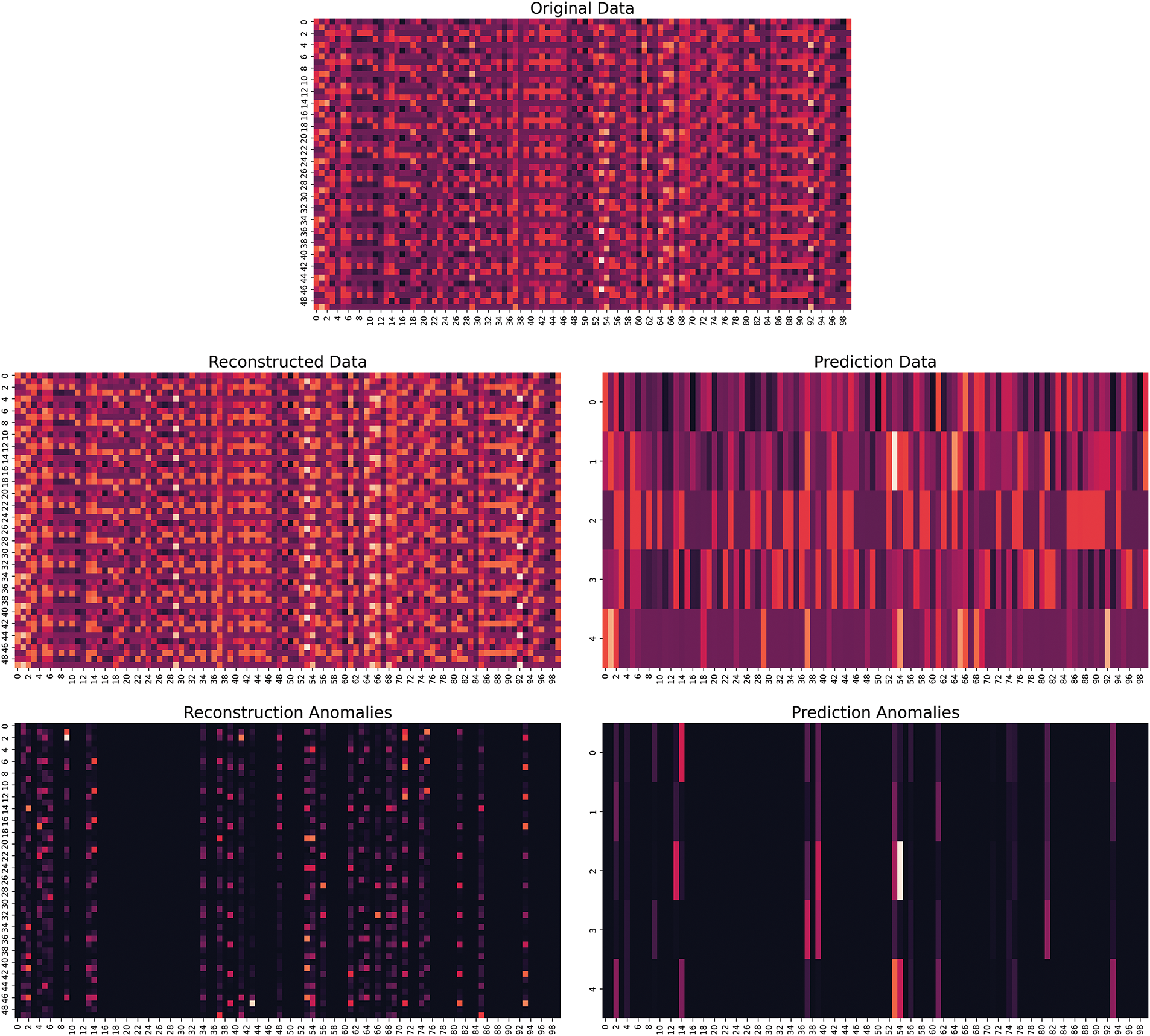
Figure 13: Anomaly detection heat map
The above images reveal that the feature data for specific time steps deviates significantly from the model’s expectations. Every image shows the features’ dimensions on the horizontal axis and their data point errors for each time step. The vertical axis in the original, reconstructed, and predicted images represents the time step index, indicating data at a specific point in time.
The Original Image shows a subset of the input data, representing multiple features within a particular time step. The brighter the color, the larger the value; the darker the color, the smaller the value. From the visual pattern of the image, it can be observed that the values of some features change regularly at specific time steps. The Reconstructed Image displays data generated by the autoencoder model, showing how the model regenerates the original data compared to the original image. Ideally, the reconstructed image should closely resemble the original image. The reconstructed and original images show almost the same pattern upon visual comparison, indicating that the model captures the standard data patterns well. However, subtle differences suggest possible anomalous regions.
Abnormal Highlights (Reconstruction) display areas with significant reconstruction errors. These are areas where the model struggles to capture data accurately during reconstruction, possibly pointing to anomalies. The brighter parts of the graph show regions with larger reconstruction errors. Some highlighted columns indicate that certain time steps combined with specific features have high reconstruction errors, which may suggest an anomaly in the data.
The prediction image shows the predictive model results, forecasting data for future time steps. From the image, we can observe that the predicted image pattern differs from the original data, suggesting that there may be anomalies at specific time steps.
We also provide partial Fig. 14 of the error generated by model anomaly detection.
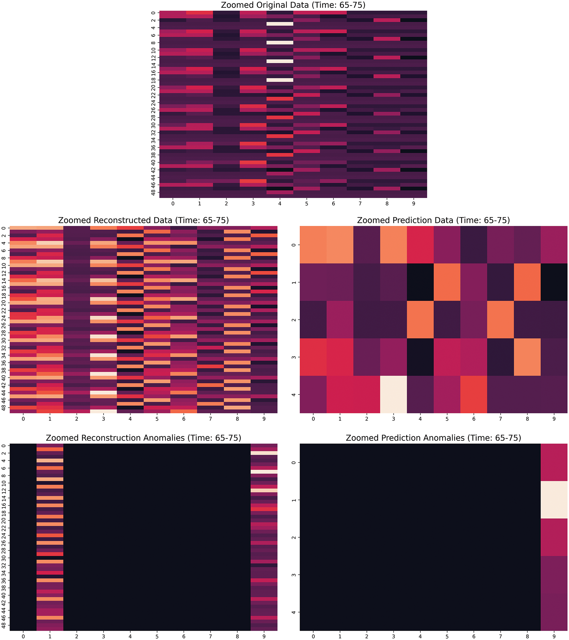
Figure 14: Analysis of model misjudgment in reconstruction and prediction anomalies
We can see that the model’s two misjudgments in time steps 65–75 are mainly due to the failure to effectively capture features with large fluctuations in the data while showing excessive sensitivity to edge features. The fourth and fifth characteristics of the raw data showed significant high-value fluctuations during this time interval. However, the reconstruction data was not accurately restored, resulting in dispersed reconstruction errors that were not recognized as anomalies. In addition, the prediction module’s future trend judgment on feature 9 is biased, resulting in a significant difference between the predicted and actual values, leading to misjudgment. The model cannot model high fluctuation regions, and edge features (such as features 0 and 9) become the focus of anomaly judgment. Therefore, improving the model’s reconstruction capabilities (such as introducing attention mechanisms) and future trend prediction capabilities, as well as optimizing feature weight allocation, will help reduce misjudgment and improve anomaly detection accuracy.
4.4 Comparison of MemAAE with Representative Models
This section presents a performance comparison between the proposed MemAAE model and nine other anomaly detection models, evaluated on two real-world datasets: Sopan-Finder and Sunalab Faro PV 2017. Table 3 reports two key evaluation metrics—accuracy and F1-score—which are essential for assessing the overall effectiveness of anomaly detection methods and the trade-off between precision and recall.
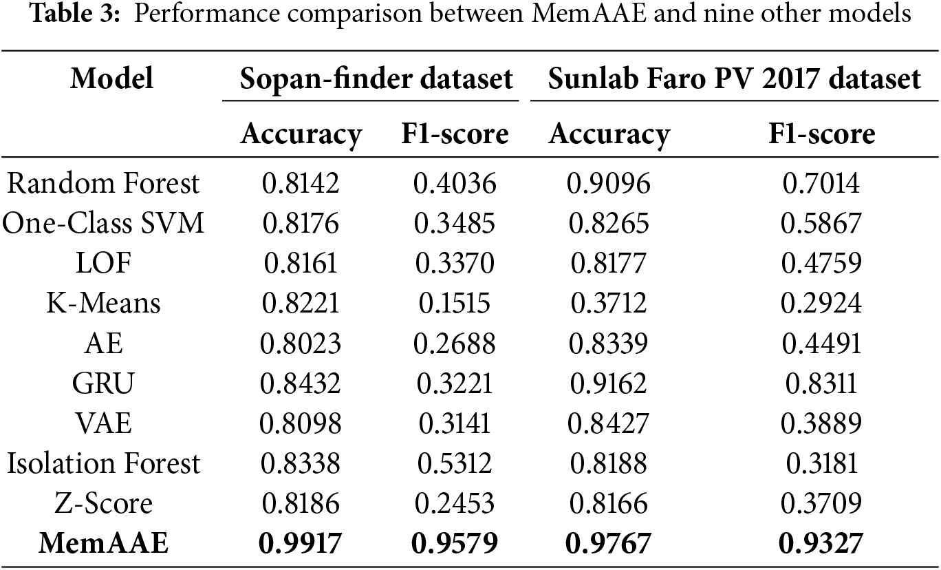
The results in Table 3 demonstrate that the MemAAE model performs exceptionally well on both datasets, significantly outperforming all comparative models. On the Sopan-Finder dataset, MemAAE achieves an accuracy of 99.17% and an F1-score of 95.79%, while on the Sunalab Faro PV 2017 dataset, it achieves an accuracy of 97.67% and an F1-score of 93.27%. In contrast, other models, such as Random Forest, GRU, and Isolation Forest, show relatively strong performance but remain slightly inferior to MemAAE overall. Furthermore, traditional methods like K-Means and One-Class SVM exhibit poorer F1-scores, underscoring their limitations in handling anomaly detection tasks.
The ROC results in Fig. 15 demonstrate that the MemAAE model achieves exceptional performance on both datasets. In the Sopan-Finder dataset, MemAAE achieves an AUC (Area Under the ROC Curve) of 0.97, showcasing its excellent ability to distinguish anomalies. Similarly, in the Sunalab Faro PV 2017 dataset, MemAAE achieves an AUC of 0.93, further validating its robustness and effectiveness in anomaly detection tasks. These results highlight the model’s capability to maintain a high true positive rate while minimizing the false positive rate.
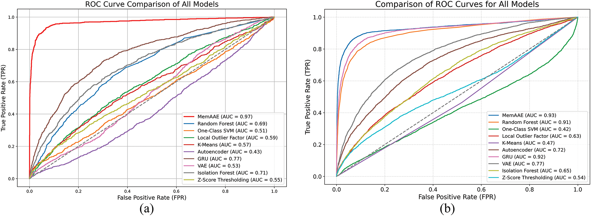
Figure 15: Comparison of roc curves for different models. (a) ROC curves of all models on the SoPan-Finder dataset. (b) ROC curves of all models on the Sunlab Faro PV 2017 dataset
Combining Table 3 and Fig. 15, we observe that the MemAAE model effectively addresses the key limitations of traditional methods by integrating reconstruction error, prediction error, and a dynamic thresholding mechanism, demonstrating exceptional performance in time series anomaly detection. The model leverages an LSTM-based autoencoder to capture temporal dependencies, ensuring low reconstruction errors for standard data, while the prediction module forecasts future trends to identify deviations effectively. A memory module with 200 slots and SoftMax-based weighting enhances the model’s ability to focus on critical patterns, improving its capacity to distinguish anomalies from standard data, something conventional LSTM and GRU models struggle to achieve. Furthermore, based on the 85th percentile of combined errors within a sliding window, the dynamic thresholding mechanism allows the model to adapt to local data fluctuations, enhancing its sensitivity to diverse anomaly patterns while reducing false detections caused by static thresholds. Robustness to complex fluctuations and edge features is further strengthened through adversarial training, enabling the model to maintain stability where traditional methods such as K-Means and Z-Score fail. Experimental results validate the effectiveness of MemAAE: it achieves an accuracy of 99.17% and an F1-score of 95.79% (AUC = 0.97) on the Sopan-Finder dataset and an accuracy of 97.67% with an F1-score of 93.27% (AUC = 0.93) on the Sunalab Faro PV 2017 dataset. These findings confirm that MemAAE achieves a higher actual positive rate (TPR) while minimizing the false positive rate (FPR), demonstrating its robustness and adaptability to dynamic and complex time series anomaly detection tasks.
We visualized the test results of all models on the Sopan-Finder Dataset. Each subplot illustrates the detected expected points (green) and anomalies (red) for a specific model and compares them with the actual label distribution (top-left) for reference, as shown in Fig. 16.


Figure 16: Visual comparison of anomaly distribution
Fig. 16 shows the relationship between temperature (°C) and PV_Demand (kW), where the outlier (red) is concentrated near zero and distributed over different temperature ranges, indicating significant anomalies in system behavior when PV_Demand is low. Our MemAAE model (LSTM-based self-encoder) can accurately identify the complex relationship between temperature fluctuations and PV_Demand anomalies by introducing memory modules to store normal data patterns efficiently. In addition, MemAAE combines reconstruction error with prediction error so that it has strong robustness and detection accuracy even when the data distribution is uneven.
MemAAE performs the best, with anomaly points being highly consistent with the real labels and demonstrating strong anomaly detection capabilities. We also present the confusion matrices of multiple models in anomaly detection tasks. The vertical axis of each confusion matrix represents the true labels, while the horizontal axis represents the model’s predicted results. By observing the performance of each model, it is possible to compare their effectiveness in detecting normal points (TN) and abnormal points (TP), as shown in Fig. 17.
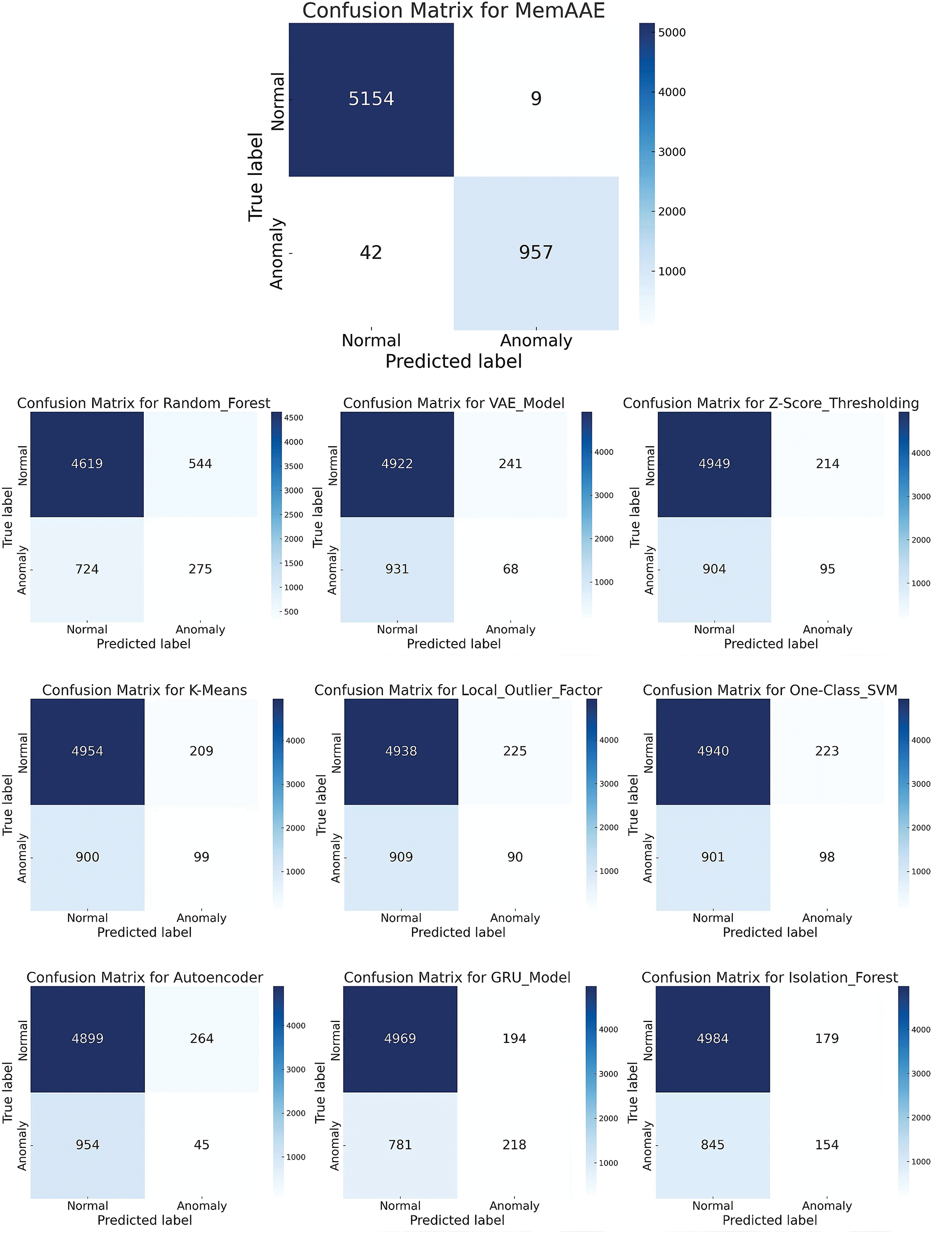
Figure 17: Confusion matrix comparison
True Negative (TN): The actual normal sample, and the model predicts the normal sample. False Positive (FP): Actual normal sample, but model error prediction as exceptional sample (false positives). False Negative (FN): Actual exception sample, but model error prediction is normal sample (missing report). True Positive (TP): The actual exception sample and the model correctly predicts the exception sample.
Based on the analysis of the confusion matrices, we can see that MemAAE model has excellent performance and high accuracy and recall rate, indicating that the model’s overall performance is stable when detecting abnormalities. Although the false positives rate is low, some exceptions (42) are missing, and in sensitive application scenarios, the omission can be reduced by adjusting the model’s threshold.
4.5 Applicability Experiments for the Proposed Module
We compared the complete MemAAE model with versions that excluded either the memory or prediction modules. When both modules are removed, the MemAAE model reverts to a standard LSTM autoencoder.
According to Table 4, memory modules significantly enhance the model’s accuracy, recall, and F1-score. Without these modules, the model’s ability to classify anomalies drops considerably, suggesting that memory modules are essential for interpreting historical data and supporting accurate anomaly detection.

The prediction module also plays a crucial role by allowing the model to forecast future values in the latent space and compare them to observed values. This approach enhances the model’s focus on current data while utilizing predictive insights for more thorough anomaly detection. The experiments confirm that removing either module alone results in a marked decline in the model’s performance, underscoring the importance of both memory and prediction modules. Consequently, maintaining both modules is crucial for effective, reliable, and accurate anomaly detection.
Memory modules are essential for the MemAAE model’s learning and anomaly detection capabilities. They allow the model to capture and retain critical information in steps of time. By adjusting the memory size, we can directly control the model’s ability to store and process information.
Naturally, different memory sizes also directly affect the model’s accuracy and overall performance in anomaly detection. To understand the impact of varying memory sizes on the model’s anomaly detection capabilities, we compare the effectiveness of different memory sizes in anomaly detection, as detailed in Fig. 18.
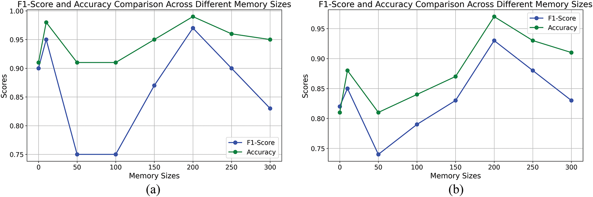
Figure 18: The impact of different memory sizes. (a) Comparison across memory sizes on the Sopan-Finder dataset. (b) Comparison across memory sizes on the Sunalab Faro PV 2017 dataset
Fig. 18 illustrates the impact of varying memory sizes on the F1-score and accuracy of the MemAAE model across two datasets. Performance exhibits fluctuations as memory size changes in the Sopan-Finder dataset (a) and the Sunalab Faro PV 2017 dataset (b). The optimal performance is achieved at a memory size of 200, with both accuracy and F1-score peak, indicating the model’s ability to capture critical patterns effectively. Beyond this point, a slight decline in performance is observed, suggesting that substantial memory sizes may introduce redundancy or overfitting. These findings underscore the importance of selecting an appropriate memory size to balance model capacity and performance.
Fig. 19 illustrates the effect of varying weighting factors on the accuracy and F1-score of the MemAAE model. Across both datasets, performance improves as the weighting factor increases, reaching its peak at 0.7. Beyond this point, a slight decline is observed, suggesting that 0.7 represents the optimal balance between reconstruction and prediction errors. This optimal weighting factor ensures the highest accuracy and F1-score, underscoring the critical importance of balancing these two error components to achieve optimal anomaly detection performance.
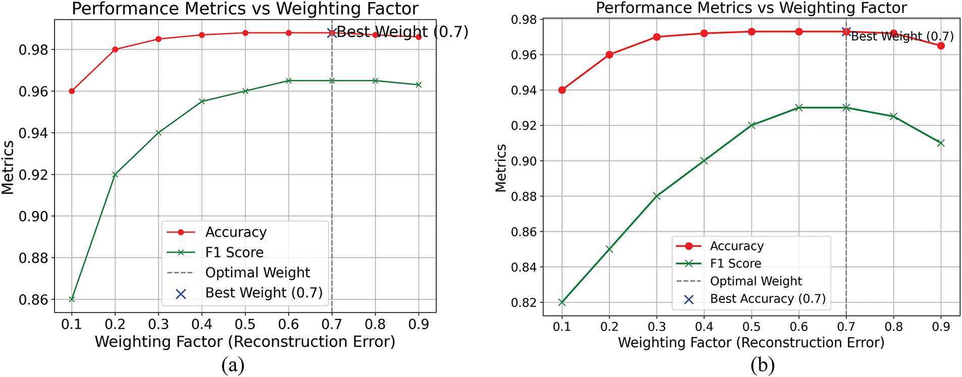
Figure 19: Comparison of weighted effect graphs for different reconstruction and prediction errors. (a) Performance metrics vs. weighting factor on the Sopan-Finder dataset. (b) Performance metrics vs. weighting factor on the Sunalab Faro PV 2017 dataset
4.8 Statistical Significance Analysis of MemAAE Performance
Fig. 20 illustrates the statistical significance analysis of the MemAAE model’s performance across the Sopan-Finder and Sunalab Faro PV 2017 datasets. The t-statistic values (blue bars) indicate significant deviations, while the—log10 (p-values) (red dashed lines) confirm the statistical significance of the results. Notably, the lower p-values, particularly in the Sopan-Finder dataset, provide strong evidence of the robustness and reliability of the MemAAE model’s performance in anomaly detection tasks.
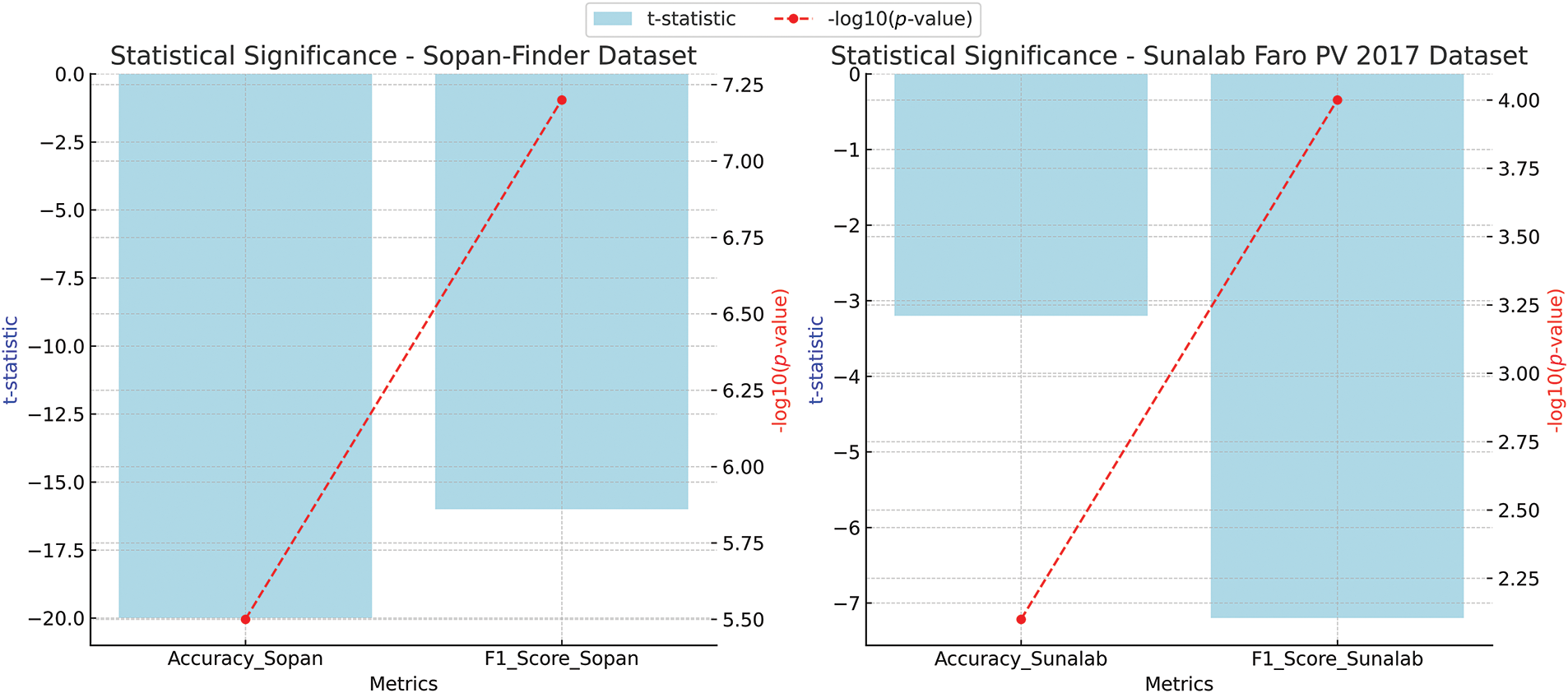
Figure 20: Comparison of t-statistic and p-values
4.9 Confidence Experiments and Confidence Intervals
In the confidence experiment, the Sopan-Finder and Sunlab Faro PV 2017 datasets were randomly selected 2000 times from the test set to evaluate the AUC, Accuracy, and F1-score distributions and corresponding 2.5% and 97.5% percentiles. As shown on Fig. 21.
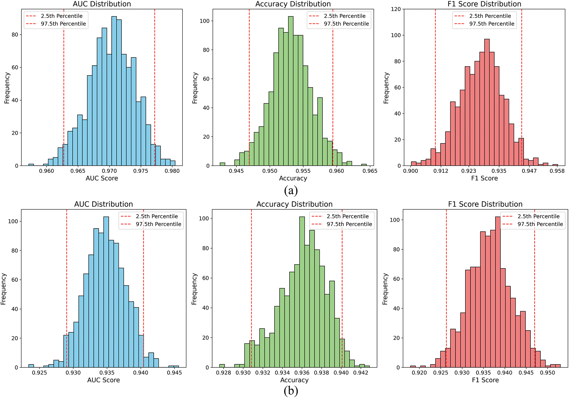
Figure 21: Confidence experiment performance metric distributions across different datasets. (a) Confidence experiment on the Sopan-Finder dataset. (b) Confidence experiment on the Sunalab Faro PV 2017 dataset
The results showed that the model performed better on the Sopan-Finder dataset than on the Sunlab Faro PV 2017 dataset, with AUC, Accuracy, and F1-score more concentrated and higher values: AUC was mainly distributed from 0.965 to 0.975, and F1-score from 0.920 to 0.940. By comparison, on the Sunlab Faro PV 2017 dataset, the AUC and Accuracy range from 0.930 to 0.940, and the F1-score ranges from 0.930 to 0.945. Overall, the confidence intervals on both data sets are narrow, indicating stable performance and reliable results. At the same time, the model’s performance on different data sets verifies its stability and generalization ability, supporting the reliable evaluation of model performance.
Future work will focus on further optimizing the performance and practical application of the MemAAE model to address current challenges related to computational overhead, lack of generalization, and real-time deployment. Firstly, the computational complexity of memory modules and adversarial training will be reduced through model pruning and quantization techniques, which will improve the efficiency of the model in real-time environments. Secondly, the validation of extended models on multiple datasets, especially tests under different climatic conditions, geographical regions, and with larger datasets, will enhance the generalization and scalability of the models.
Additionally, to further enhance model robustness, advanced attention mechanisms and multi-variable memory modules will be integrated. These techniques will help reduce the impact of large data fluctuations by focusing on the most relevant features in the time series data, improving the model’s ability to capture long-range dependencies and mitigate noise. By applying attention mechanisms, the model can better allocate its focus to critical anomalies, while a multi-variable memory module can help preserve important contextual information across different variables, making the system more resilient to data volatility.
At the same time, future research will drive the practical deployment and integration of models, combining SCADA systems and existing VPP management platforms for field testing to assess their stability and performance in industrial environments. Furthermore, the interpretability of the model will be a key focus, making detection results more transparent through visualization tools and feature importance analysis, which will aid in the construction of decision support systems. Finally, more advanced deep learning methods such as Variational Autoencoders (VAE), Graph Neural Networks (GNN), and Transformer models will be explored further to improve anomaly detection in complex time series data.
This paper presents a hybrid memory-enhanced adversarial autoencoder (MemAAE) model for virtual power plant (VPP) anomaly detection by combining an LSTM self-encoder, memory module, adversarial training, and prediction module. The MemAAE model improves the detection capability of complex anomalies by combining reconstruction error and prediction error. The dynamic threshold mechanism is based on the 85-quadrant adaptive adjustment of the sliding window. In addition, the memory module captures critical normal patterns through 200 memory slots and SoftMax weighting mechanisms, improving the model’s ability to distinguish between normal and abnormal data.
Experimental results show that MemAAE performs well on both real-world solar power datasets. On the Sopan-Finder dataset, MemAAE achieved 99.17% accuracy, an F1-score of 95.79%, and an AUC of 0.97. On the Sunalab Faro PV 2017 dataset, MemAAE achieved 97.67%, an F1-score of 93.27%, and an AUC of 0.93. These results demonstrate MemAAE’s effectiveness and robustness in time-series anomaly detection tasks while outperforming various benchmark models, including Random Forest, GRU, and Isolation Forest.
Further experiments and visualizations reveal the effect of different memory sizes and weighting factors on model performance. The model’s performance is optimal when the memory size is 200, and the reconstruction error is 0.7. This reflects MemAAE’s ability to balance reconstruction errors with prediction errors and the effectiveness of memory modules in capturing key features.
However, there are certain limitations to consider. The memory module introduces additional computational overhead, which could affect real-time deployment, particularly in large-scale VPP systems. The memory size, while critical to model performance, can lead to overfitting when excessively large, especially in datasets with a high anomaly rate, where the model might excessively memorize normal data patterns. Additionally, the dynamic nature of real-time anomaly detection might be impacted by these factors, potentially limiting the model’s practical application in highly volatile environments.
The dataset and code for this experiment are available on GitHub: https://github.com/kikigo201012/Solar-Time-Series-Anomaly-Detection-Codes-and-Datasets-Based-on-MemAAE-Model (accessed on 15 December 2024).
Acknowledgement: We want to extend our heartfelt gratitude to everyone who contributed to the success of this research. First and foremost, we thank our colleagues and collaborators for their valuable discussions and insights, which significantly enhanced the quality of our work. We are also grateful to the editorial team and the anonymous reviewers for their constructive feedback and suggestions, which helped us to refine and improve this manuscript. Special thanks go to our institutions for the technical and financial support that enabled us to conduct this research. Finally, we thank our families and friends for their unwavering support and encouragement throughout this project.
Funding Statement: This research was supported by “Regional Innovation Strategy (RIS)” through the National Research Foundation of Korea (NRF) funded by the Ministry of Education (MOE) (2021RIS-002) and the Technology Development Program (RS-2023-00266141) funded by the Ministry of SMEs and Startups (MSS, Republic of Korea).
Author Contributions: Study conception and design: Yuqiao Liu, Chang Gyoon Lim; Data collection: Yuqiao Liu; Data processing and preparation: Chen Pan; Analysis and interpretation of results: Yuqiao Liu, Chen Pan, Chang Gyoon Lim; Draft manuscript preparation: Yuqiao Liu, YeonJae Oh; Funding acquisition: YeonJae Oh, Chang Gyoon Lim. All authors reviewed the results and approved the final version of the manuscript.
Availability of Data and Materials: The authors confirm that the data supporting the findings of this study are available within the article.
Ethics Approval: Not applicable.
Conflicts of Interest: The authors declare no conflicts of interest to report regarding the present study.
Nomenclature
| Mean of the feature values | |
| The standard deviation of the feature values | |
| MSE | Mean squared error |
| AUC | The area under the ROC curve |
| TP | True positives |
| FP | False positives |
| FN | False negatives |
| TN | True negatives |
| F1 | F1-score, the harmonic means of precision and recall. |
| Predicted value | |
| Actual value | |
| Dynamic threshold | |
| Error for a given data point | |
| Weights of the discriminator | |
| Real data loss | |
| Fake data loss | |
| Weights of the output gate | |
| Bias of the output gate | |
| Output from the output gate | |
| Hidden state at time step | |
| Cell state after forget gate control | |
| Weights of the forget gate | |
| Bias of the forget gate | |
| Predicted outcome | |
| PV_Demand | Photovoltaic power demand |
| temp | Temperature |
| Table of Mathematical Variables and Notations | |
| Symbol/Abbreviation | Description |
| Raw data matrix | |
| Mean of the feature values | |
| The standard deviation of each feature | |
| Standardized data matrix | |
| Size of the sliding window | |
| Starting index of the window | |
| Hidden state at time step | |
| Cell state at the time step | |
| Activation value of the forget gate | |
| Candidate cell state in the input gate | |
| Activation value of the input gate | |
| Activation value of the output gate | |
| Reconstructed data point | |
| Hidden state output by the LSTM | |
| Memory slot | |
| Attention weight for memory vector | |
| Weighted memory module output | |
| Discriminator output probability | |
| Reconstruction loss function | |
| Generator adversarial loss | |
| Combined loss function | |
| Predicted value at time step | |
| Actual value at time step | |
| Reconstruction error | |
| Prediction error | |
| Dynamic threshold for partition | |
| Predicted anomaly label | |
| Error for data point | |
| True Positives (correctly classified anomalies) | |
| True Positives (correctly classified anomalies) | |
| False Positives (incorrectly classified normal points) | |
| False Negatives (incorrectly classified anomalies) | |
References
1. Abdelkader S, Amissah J, Abdel-Rahim O. Virtual power plants: an in-depth analysis of their advancements and importance as crucial players in modern power systems. Energ Sustain Soc. 2024;14(1):52. doi:10.1186/s13705-024-00483-y. [Google Scholar] [CrossRef]
2. Taheri SI, Wolter Ferreira Touma D, de Salles MBC. Virtual power plants for smart grids containing renewable energy. In: Smart grids—renewable energy, power electronics, signal processing and communication systems applications. Cham: Springer International Publishing; 2023. p. 173–94. doi: 10.1007/978-3-031-37909-3_6. [Google Scholar] [CrossRef]
3. Liu J, Hu H, Yu SS, Trinh H. Virtual power plant with renewable energy sources and energy storage systems for sustainable power grid-formation, control techniques and demand response. Energies. 2023;16(9):3705. doi:10.3390/en16093705. [Google Scholar] [CrossRef]
4. Strezoski L, Padullaparti H, Ding F, Baggu M. Integration of utility distributed energy resource management system and aggregators for evolving distribution system operators. J Mod Power Syst Clean Energy. 2022;10(2):277–85. doi:10.35833/MPCE.2021.000667. [Google Scholar] [CrossRef]
5. Tan Z, Zhong H, Xia Q, Kang C, Wang XS, Tang H. Estimating the robust P-Q capability of a technical virtual power plant under uncertainties. IEEE Trans Power Syst. 2020;35(6):4285–96. doi:10.1109/TPWRS.2020.2988069. [Google Scholar] [CrossRef]
6. Bagal KN, Kadu CB, Vikhe PS, Parvat BJ. PLC based real time process control using SCADA and MATLAB. In: 2018 Fourth International Conference on Computing Communication Control and Automation (ICCUBEA); 2018; IEEE. doi:10.1109/ICCUBEA.2018.8697491. [Google Scholar] [CrossRef]
7. Vale ZA, Morais H, Silva M, Ramos C. Towards a future SCADA. In: 2009 IEEE Power & Energy Society General Meeting; 2009 Jul 26–30; Calgary, AB, Canada: IEEE; 2009. p. 1–7. doi:10.1109/PES.2009.5275561. [Google Scholar] [CrossRef]
8. Aghenta LO, Iqbal MT. Low-cost, open source IoT-based SCADA system design using Thinger.IO and ESP32 thing. Electronics. 2019;8(8):822. doi:10.3390/electronics8080822. [Google Scholar] [CrossRef]
9. Eden P, Blyth A, Jones K, Soulsby H, Burnap P, Cherdantseva Y, et al. SCADA system forensic analysis within IIoT. In: Cybersecurity for Industry 4.0: Analysis for Design and Manufacturing. Springer Series in Advanced Manufacturing. Cham: Springer; 2017. p. 73–101. doi:10.1007/978-3-319-50660-9_4. [Google Scholar] [CrossRef]
10. Jusoh W, Hanafiah MA, Ghani MR, Raman SH. Remote terminal unit (RTU) hardware design and implementation efficient in different application. In: 2013 IEEE 7th International Power Engineering and Optimization Conference (PEOCO); 2013; IEEE. doi: 10.1109/PEOCO.2013.65.64612. [Google Scholar] [CrossRef]
11. Patel SC, Sanyal P. Securing SCADA systems. Inf Manag Comput Secur. 2008;16(4):398–414. doi:10.1108/09685220810908804. [Google Scholar] [CrossRef]
12. Wang K, Gou C, Duan Y, Lin Y, Zheng X, Wang FY. Generative adversarial networks: introduction and outlook. IEEE/CAA J Autom Sinica. 2017;4(4):588–98. doi:10.1109/JAS.2017.7510583. [Google Scholar] [CrossRef]
13. Sakurada M, Yairi T. Anomaly detection using autoencoders with nonlinear dimensionality reduction. In: Proceedings of the MLSDA 2014 2nd Workshop on Machine Learning for Sensory Data Analysis; 2014; Gold Coast Australia QLD Australia: ACM. p. 4–11. doi:10.1145/2689746. [Google Scholar] [CrossRef]
14. Fisch ATM, Eckley IA, Fearnhead P. A linear time method for the detection of point and collective anomalies. arXiv:1806.01947. 2018. [Google Scholar]
15. Yuan L, Ye F, Li H, Zhang C, Gao C, Yu C, et al. Semi-supervised anomaly detection with contamination-resilience and incremental training. Eng Appl Artif Intell. 2024;138(10):109311. doi:10.1016/j.engappai.2024.109311. [Google Scholar] [CrossRef]
16. Smith SM, Nichols TE. Threshold-free cluster enhancement: addressing problems of smoothing, threshold dependence and localisation in cluster inference. NeuroImage. 2009;44(1):83–98. doi:10.1016/j.neuroimage.2008.03.061. [Google Scholar] [PubMed] [CrossRef]
17. Park H, Noh J, Ham B. Learning memory-guided normality for anomaly detection. In: IEEE/CVF Conference on Computer Vision and Pattern Recognition (CVPR); 2020 Jun 13–19; Seattle, WA, USA: IEEE; 2020. p. 14360–9. doi:10.1109/cvpr42600.2020.01438. [Google Scholar] [CrossRef]
18. Gong D, Liu L, Le V, Saha B, Mansour MR, Venkatesh S, et al. Memorizing normality to detect anomaly: memory-augmented deep autoencoder for unsupervised anomaly detection. In: 2019 IEEE/CVF International Conference on Computer Vision (ICCV); 2019 Oct 27–Nov 2; Seoul, Republic of Korea: IEEE; 2019. p. 1705–14. doi:10.1109/iccv.2019.00179 [Google Scholar] [CrossRef]
19. Shafahi A, Najibi M, Ghiasi A, Xu Z, Dickerson J, Studer C, et al. Adversarial training for free!. arXiv:1904.12843. 2019. [Google Scholar]
20. Zamanzadeh Darban Z, Webb GI, Pan S, Aggarwal C, Salehi M. Deep learning for time series anomaly detection: a survey. ACM Comput Surv. 2024;57(1):1–42. doi:10.1145/3691338. [Google Scholar] [CrossRef]
21. Ul Hassan M, Rehmani MH, Chen J. Anomaly detection in blockchain networks: a comprehensive survey. IEEE Commun Surv Tutorials. 2023;25(1):289–318. doi:10.1109/COMST.2022.3205643. [Google Scholar] [CrossRef]
22. Chaovalitwongse WA, Fan YJ, Sachdeo RC. On the time series k-nearest neighbor classification of abnormal brain activity. IEEE Trans Syst Man Cybern Part A Syst Hum. 2007;37(6):1005–16. doi:10.1109/TSMCA.2007.897589. [Google Scholar] [CrossRef]
23. Breunig MM, Kriegel HP, Ng RT, Sander J. LOF: identifying density-based local outliers. In: Proceedings of the 2000 ACM SIGMOD International Conference on Management of Data; 2000; Dallas, TX, USA: ACM; p. 93–104. doi:10.1145/342009.335388. [Google Scholar] [CrossRef]
24. Choi K, Yi J, Park C, Yoon S. Deep learning for anomaly detection in time-series data: review, analysis, and guidelines. IEEE Access. 2021;9:120043–65. doi:10.1109/ACCESS.2021.3107975. [Google Scholar] [CrossRef]
25. Miao J, Tao H, Xie H, Sun J, Cao J. Reconstruction-based anomaly detection for multivariate time series using contrastive generative adversarial networks. Inf Process Manag. 2024;61(1):103569. doi:10.1016/j.ipm.2023.103569. [Google Scholar] [CrossRef]
26. Chung J, Gulcehre C, Cho K, Bengio Y. Empirical evaluation of gated recurrent neural networks on sequence modeling. arXiv:1412.3555. 2014. [Google Scholar]
27. Lee B, Kim S, Maqsood M, Moon J, Rho S. Advancing autoencoder architectures for enhanced anomaly detection in multivariate industrial time series. Comput Mater Contin. 2024;81(1):1275–300. doi:10.32604/cmc.2024.054826. [Google Scholar] [CrossRef]
28. Ergen T, Kozat SS. Unsupervised anomaly detection with LSTM neural networks. IEEE Trans Neural Netw Learning Syst. 2020;31(8):3127–41. doi:10.1109/TNNLS.2019.2935975. [Google Scholar] [PubMed] [CrossRef]
29. Lin C, Du B, Sun L, Li L. Hierarchical context representation and self-adaptive thresholding for multivariate anomaly detection. IEEE Trans Knowl Data Eng. 2024;36(7):3139–50. doi:10.1109/TKDE.2024.3360640. [Google Scholar] [CrossRef]
30. Yang X, Howley E, Schukat M. Agent-based dynamic thresholding for adaptive anomaly detection using reinforcement learning. Neural Comput Appl. 2024;2024(1):1–17. doi:10.1007/s00521-024-10536-0. [Google Scholar] [CrossRef]
31. Zhang Y, Wang J, Chen Y, Yu H, Qin T. Adaptive memory networks with self-supervised learning for unsupervised anomaly detection. IEEE Trans Knowl Data Eng. 2023;35(12):12068–80. doi:10.1109/TKDE.2021.3139916. [Google Scholar] [CrossRef]
32. Chang CH, Deng X, Theofanous TG. Direct numerical simulation of interfacial instabilities: a consistent, conservative, all-speed, sharp-interface method. J Comput Phys. 2013;242(11):946–90. doi:10.1016/j.jcp.2013.01.014. [Google Scholar] [CrossRef]
33. Venkatesh S, Rosin PL. Dynamic threshold determination by local and global edge evaluation. Graph Models Image Process. 1995;57(2):146–60. doi:10.1006/gmip.1995.1015. [Google Scholar] [CrossRef]
Cite This Article
 Copyright © 2025 The Author(s). Published by Tech Science Press.
This work is licensed under a Creative Commons Attribution 4.0 International License , which permits unrestricted use, distribution, and reproduction in any medium, provided the original work is properly cited.
 Downloads
 Citation Tools