SFPBL: Soft Filter Pruning Based on Logistic Growth Differential Equation for Neural Network

1  Introduction

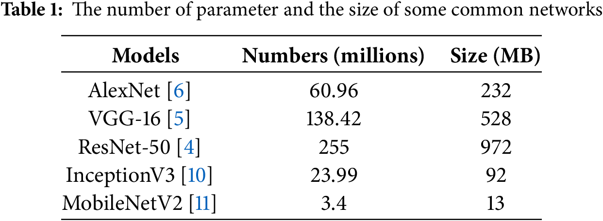
Convolutional Neural Networks (CNN) [1] has achieved remarkable results in various tasks of computer vision such as object detection [2,3], image classification [4–7], and semantic segmentation [8,9]. However, as networks become more profound and complex, they often suffer from over-parameterization, where the network contains more parameters than necessary to achieve optimal performance. This increases the model size and can lead to over-fitting, reducing the generalization capability of the network. Furthermore, larger model sizes pose challenges in deployment and operation, particularly in resource-constrained environments. The number of parameters in a neural network is typically a key metric for measuring model size. The number of parameters and the network’s size can be estimated from the network structure and weights. Table 1 shows the parameter count and size of some common network architectures, highlighting the tendency for modern networks to grow significantly in size as they seek higher accuracy.

•   Neural Network Quantization [12]: This technique involves converting the floating-point parameters in a neural network to lower-precision data types, such as converting 32-bit floating-point numbers to 16-bit or 8-bit integers, reducing the size of the neural network.

•   Knowledge Distillation [13,14]: Utilizing a more extensive pre-trained neural network to guide and train a smaller neural network to capture the knowledge from the pre-trained network, resulting in a smaller neural network.

•   Structural Optimization: Optimizing the structure of a neural network, such as decreasing redundant layers, merging specific layers, etc., to reduce the complexity of the neural network.

•   Neural Network Compression: Employing specialized neural network compression techniques, such as NVIDIA’s TensorRT [15], Google’s Android Neural Networks API (NNAPI) [16], to reduce the model file size and accelerate inference.

•   Network Pruning: Eliminating unimportant weight parameters or pruning some layers and channels in the network, a lower complexity neural network can be obtained.

Compared with other optimization techniques, pruning reduces the size of the network while maintaining its structure. Network pruning reduces model size by removing unimportant parameters while maintaining the hierarchical structure and topological connections, and it can prevent significant changes in the overall model structure. The model’s performance and generalization ability are maintained. Moreover, pruning can be flexibly adjusted according to practical applications, allowing for selecting different pruning strategies and methods. For example, pruning can be adjusted based on the resource limitations and performance requirements of the resource-constrained device, resulting in lightweight models suitable for real-world applications.

Many network pruning techniques [17–20] involve calculating the importance of filters or connections and pruning network based on specific criteria. Pruning techniques are divided into two main types: Hard Filter Pruning (HFP) [21] and Soft Filter Pruning (SFP) [17]. HFP removes specific weight parameters from the network with importance below a certain threshold, setting them to zero or deleting entire channels or layers. HFP significantly impacts the model as it directly eliminates portions of parameters or structures to reduce the network’s size. Excessive HFP may lead to a significant decrease in performance.

On the other hand, SFP scales or adjusts parameters during the pruning process rather than directly setting them to zero. SFP typically employs specific pruning strategies, such as L1 regularization [21] or the sensitivity of weight parameters. However, it requires more parameter adjustments and thus incurs higher costs. Asymptotic Soft Filter Pruning (ASFP) [18] is a well-known SFP algorithm. In ASFP [18], filters selected for pruning are set to zero in the current training epoch but are updated in the subsequent epoch to maintain their representational capacity. There is a noticeable accuracy drop during the initial pruning phase of SFP [17]. ASFP [18] mitigates this by gradually increasing the pruning rate.

To better utilize trained pruned filters, SofteR Filter Pruning (SRFP) [19] and Asymptotic SofteR Filter Pruning (ASRFP) [19] have been proposed. They employ a progressive decay method, where weights gradually approach zero. Additionally, the progressive method first prunes a small portion of filters and then prunes more during training. This progressive pruning method ensures that information is gradually concentrated in the remaining filters, stabilizing the subsequent training and pruning process.

However, due to coarse control over the attenuation process, soft pruning and its variant algorithms still cause information loss in the network, which affects its performance. To address these challenges, this study proposes a more refined control over the pruning process using a differential equation model-the Logistic Growth Differential Equation. This approach aims to mitigate the over-parameterization problem by precisely controlling the weight decay process. A weight-adaptive attenuation method is proposed to control the attenuation process and further maintain the classification accuracy of the network model.

The Soft Filter Pruning Based on Logistic Growth Differential Equation for Neural Network (SFPBL) consists of four steps: Filter Selection, Weight Attenuation, Model Training, and Filter Removal. (1) Filter Selection: In this step, filters are selected based on the L2 norm of all filters in the network, with lower norms undergoing the attenuation process. (2) Weight Attenuation: The selected filters undergo weight attenuation using a three-stage adaptive attenuation formula derived from the Logistic Growth Differential Equation. (3) Model Training: The model is retrained with forward and backward propagation after weight attenuation. (4) Filter Removal: After multiple epochs of the above steps, the network training is completed, and filters with norm “0-value” are eventually removed.

The main innovations of this paper are:

1.    Adoption of Soft Pruning Strategy: Using a soft pruning strategy ensures that the performance of the pruned network does not significantly decrease.

2.    Three-Stage Adaptive Attenuation based on the solution of Logistic Growth Differential Equation: a three-stage adaptive attenuation method based on the Logistic Growth Differential Equation is proposed, which consists of the Initial Training Stage, Rapid Attenuation Stage, and Weight Convergence Stage. It prevents the loss of effective information in the network.

3.    Superior Experimental Results: Experimental results on the CIFAR-10 [22] and ILSVRC-2012 [23] datasets demonstrate overall superiority compared to algorithms such as SFP [17], ASFP [18], SRFP [19], ASRFP [19].

In real-world scenarios, such as autonomous driving, medical imaging, and mobile augmented reality, efficient and accurate deep learning models are critical. The Soft Filter Pruning Based on the Logistic Growth Differential Equation proposed in this study allows for scalable deployment without sacrificing accuracy, making them essential tools for modern AI applications.

2  Related Work

SFP [17]: Soft Filter Pruning (SFP) is a technique aimed at reducing the complexity of neural networks while maintaining their performance. Unlike hard pruning, which involves the direct removal of certain network weights or structures, soft pruning techniques typically employ a gradual reduction of weights, allowing for a more controlled and less disruptive adjustment of the network. By scaling down or attenuating weight parameters, soft pruning methods aim to preserve the overall structure and functionality of the model while effectively reducing computational requirements. The advantages of soft pruning lie in its flexibility; it can adaptively adjust based on the training process, minimizing performance loss and facilitating the preservation of essential features in the model. Various strategies have been proposed, such as using L1 or L2 regularization to guide the pruning process. Soft pruning has proven effective across a range of network architectures, leading to lightweight yet robust models, especially suitable for deployment in resource-constrained environments. ASFP[18]: ASFP extends the principles of soft filter pruning by incorporating asymptotic behaviour in the pruning process. Unlike traditional soft pruning, which relies on a linear or exponential decay of filter weights, ASFP employs an asymptotic decay approach, allowing for an adaptive and non-linear reduction of weights over time. This method ensures critical filters experience slower attenuation while less significant ones decay faster, preventing valuable information loss. ASFP is particularly useful in scenarios where the importance of the filter varies significantly across different layers. By carefully balancing the attenuation rate, ASFP can maintain higher accuracy levels while effectively pruning filters, leading to lightweight models that retain high performance even after significant size reductions. SRFP and ASRFP [19]: SofteR Filter Pruning (SRFP) and Asymptotic SofteR Filter Pruning (ASRFP) are notable advancements in the domain of soft pruning algorithms. Both methods introduce a progressive strategy for weight attenuation, allowing the pruning process to be executed in stages, which mitigates the abrupt loss of information. In SRFP, filter weights considered less critical are gradually decayed instead of being abruptly zeroed out. This gradual reduction helps concentrate information in the remaining filters, leading to stable performance even during the pruning phase. ASRFP enhances this concept by incrementally increasing the pruning rate as training progresses, allowing for more refined control over the pruning dynamics. These methods aim to improve earlier pruning techniques by providing smoother transitions and better preserving the network’s representational capacity during pruning. SRFP and ASRFP have outperformed traditional soft pruning methods, particularly regarding accuracy retention and the ability to handle deeper neural networks.

3  Methodlogy

This method utilizes the logistic growth differential equation solution to regulate the filter weights’ decay rate precisely. The logistic growth differential equation is commonly used to model a species’ population dynamics. The population’s growth curve can be categorized into five stages: Initial, Acceleration, Turning, Slowdown, and Saturation.

1.    Initial Stage: At the beginning, the population is small and relatively sparse compared to the environmental population density, and the population growth is slow.

2.    Acceleration Stage: As the population increases, the growth rate of the population also accelerates.

3.    Turning Stage: The growth rate of the population reaches its maximum, and the population size at this point is half of the saturation quantity.

4.    Slowdown Stage: Influenced by environmental and resource factors, the growth rate of the population slows down.

5.    Saturation Stage: The population reaches its maximum size and tends to saturate.

Compared to the SFP [17], which directly removes filters and the imprecise control over weight attenuation in SRFP [19] and ASRFP [19], this paper employs the logistic growth differential equation to the attenuation process of model filter weights. It can enable a more accurate simulation of the attenuation process and more precise control of filter weights. As shown in Fig. 1, the algorithm consists of four steps:

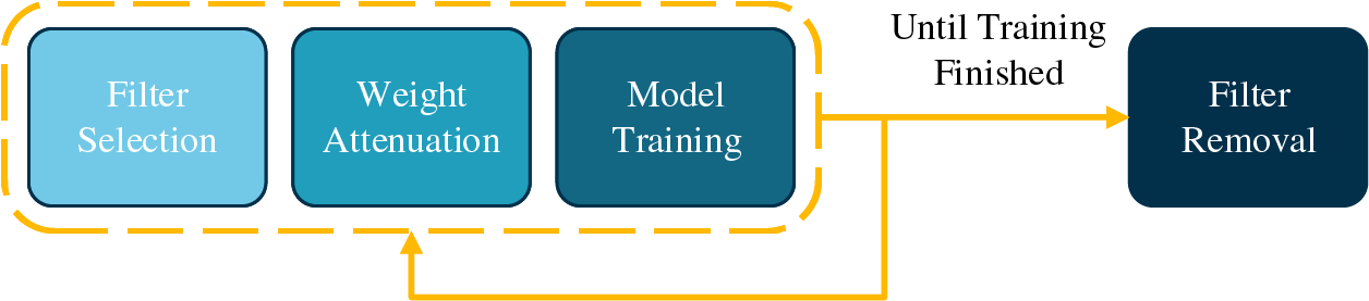
Figure 1: Overall module framework diagram of the method

1.    Filter Selection: Based on the L2 norm of filter weight in the network, filters with lower norms are selected for the second step of weight attenuation.

2.    Weight Attenuation: According to the solution of the logistic growth differential equation and the L2 norm [17] of the filter weight, the weights of the selected filters are attenuated adaptively.

3.    Model Training: After the attenuation, the network model undergoes another forward and backward propagation.

4.    Filter Removal: Filters with norm zero weights are removed through multiple iterations of the above three steps until the network training is completed.

Filter Selection: To evaluate the importance of filters, the L2 norm [21] is adopted as shown in Eq. (1), where represents the weight parameter of the j-th filter in the i-th layer of the network. The L2 norm provides a single scalar value that reflects the overall contribution of that filter to the feature extraction process.

(1)

Using the L2 norm allows for a straightforward comparison of the relative importance of different filters within a layer. Filters with smaller L2 norm values have lower magnitudes, suggesting they contribute less to the network’s final output. Thus, pruning operations target these lower-value filters, prioritizing those with more minor L2 norms. This selection process is crucial because it minimizes the impact on the network’s performance while reducing complexity.

To carry out the filter selection, a threshold-based approach is often employed. The L2 norms of all filters in a given layer are computed and sorted in ascending order. A predefined pruning ratio or threshold is then used to determine which filters fall below a specific L2 norm value and are eligible for pruning. For example, if a 30% pruning rate is selected for a particular layer, the bottom 30% of filters, based on their L2 norm ranking, will be chosen for the attenuation and pruning process. This method ensures that filters with higher L2 norms, likely to capture more significant features, are retained.

Weight Attenuation: The logistic growth differential equation is traditionally used to describe an independent biological population. Let be a change rate of population size, which linearly decreases as the population size increases. Here, time is represented by t and the maximum value of the population by . When the population size , the change rate is set to . When the population size reaches its maximum value , the rate of change becomes 0 because the population size cannot increase any further, and can be expressed by Eq. (2).

(2)

According to the initial assumption, as the population increases, the change rate decreases linearly. Therefore, the rate can be calculated as Eq. (3).

(3)

So, within any given time interval , the change in the population’s count is described by Eq. (4).

(4)

Taking to approach 0, the resulting differential equation is shown in Eq. (5).

(5)

Substituting the expression for from Eq. (3) into Eq. (5) and simplifying, the logistic growth differential equation is formulated as Eq. (6).

(6)

Integrating both sides of Eq. (6) indefinitely and simplify, yielding Eq. (7) as shown.

(7)

Its solution is shown in Eq. (8), where C is an arbitrary constant.

(8)

To visually depict the characteristics of the solution of the logistic growth differential equation, the curve described by Eq. (8) is illustrated in Fig. 2. From Fig. 2, it can be observed that the solution exhibits the following features: slow growth at the beginning, followed by rapid growth in the middle, and eventually approaching a plateau towards the end. Considering that the logistic growth differential equation represents an increasing curve while an attenuation process is required in the pruning algorithm, Eq. (8) is reformulated as Eq. (9):

(9)

where represents the attenuation rate at training epoch t. It achieves a progressive attenuation effect by multiplying the weights of the selected filters. In the attenuation process, the initial value of the attenuation rate is set to the maximum, . Through iterative training of the network, the attenuation coefficient gradually approaches zero. Additionally, certain filters will be removed after the network training to obtain the final lightweight model. When the attenuation rate drops below a threshold , it is directly replaced with zero.

Figure 2: Logistic Growth Differential Equation and norm distribution range

In the process of pruning deep neural networks, pruning strategies are typically adjusted dynamically according to the network’s training phase and the weights’ characteristics. In the initial phase, the network contains many redundant weights and unnecessary parameters, which affect the model’s computational efficiency and memory usage. Therefore, a higher pruning rate is applied in this stage to quickly remove these unimportant parameters, aiming to reduce the computational burden and enhance the model’s efficiency. Since redundancy is prevalent at this stage, pruning must be maintained for a prolonged period to ensure that most redundant weights are effectively removed, preventing premature pruning. To achieve this, a higher pruning rate is maintained for an extended period in the early stage until the redundant weights are sufficiently cleared.

In the second phase, after most of the redundant weights are pruned, the remaining weights are generally more critical and play a significant role in the model’s performance. As a result, the pruning rate needs to be reduced quickly to avoid accidentally removing important weights. If the pruning rate remains too high, it could lead to the excessive pruning of essential weights, thus severely degrading the model’s performance. Therefore, the pruning rate must be reduced rapidly and approach zero, safeguarding the network’s most important parameters.

In the final pruning phase, most redundant parameters have already been removed, and the pruning process is nearing completion. At this point, the pruning rate is kept at a low level to tune the final stages of pruning finely. This ensures that, while minimizing the number of parameters and computational load, the model’s performance is not compromised.

Our proposed pruning algorithm leverages the logistic growth differential equation in Eq. (9) to control the decay rate during different training stages precisely. In the early phase, a higher pruning rate facilitates the rapid removal of redundant parameters; in the second phase, the pruning rate is gradually reduced to avoid the loss of critical weights; and in the final stage, a low pruning rate is maintained to optimize the network structure. This process aligns well with the function curve described in Eq. (9), demonstrating the algorithm’s ability to manage the pruning rate at various stages of training dynamically.

The hyperparameters C and in Eq. (9) will be determined in subsequent experiments. Therefore, it can be observed that this calculation is only related to the training epochs.

Meanwhile, two phenomena may exist in the actual network training: (1) The norm values of all filters in a convolutional layer of the network are close; (2) The norms of filters with lower importance in a specific convolutional layer are not close to zero. For the first case, the minor difference between the maximum and minimum norms will be used to select pruning filters with an appropriate degree. In the second case, excessive decay of filter weights with more minor but non-zero norms may result in the loss of valuable information, directly impacting the model’s classification accuracy.

To address these challenges, we incorporate the L2 norm of the filter weight in the calculation formula for the attenuation rate, using it as the second factor. Consequently, the attenuation rates of different filters are adaptively adjusted based on their norms. The calculation of in Eq. (9) is expanded into the form of a two-dimensional matrix and incorporates weight norms , as shown in Eq. (10).

(10)

where is the L2 norm of the filter weight. Thus, the weight is updated by Eq. (11).

(11)

where is a two-dimensional matrix composed of a series of zeros and ones, matching the dimensions of the weight matrix . When , it is equivalent to performing the zeroing operation on the filters. Conversely, when , no operation is performed on the filter. is the attenuation rate for the j-th filter in the i-th layer. The hard pruning is obtained if each is set to zero. Each is initially set to a non-zero value. Fig. 3 illustrates one iteration of the pruning process of the proposed method.

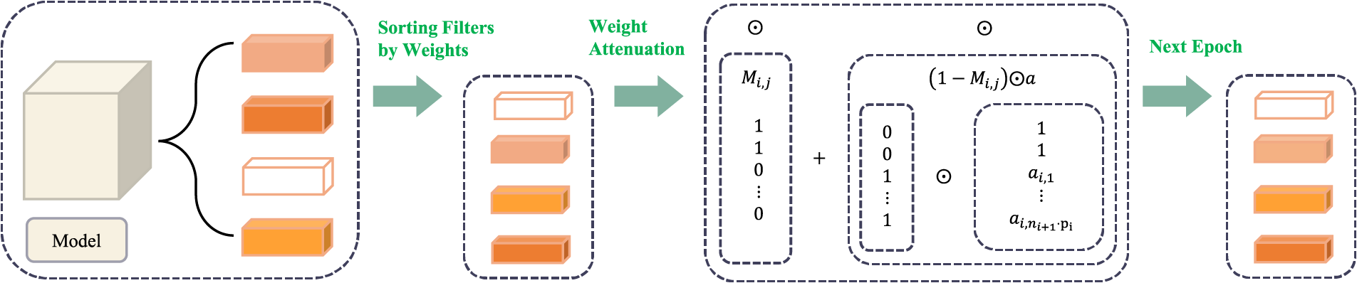
Figure 3: Pruning process of SFPBL

Model Training: After each training epoch, the network undergoes an attenuation operation, followed by the next epoch’s training. This process is repeated until the network reaches convergence. The attenuation rate curve is shown in Fig. 4, which can be divided into three distinct stages during the pruning process: the initial training stage, rapid attenuation stage, and weight convergence stage. In the initial training stage, the change in decay rate is minimal. This slow decay is intentional, as it helps preserve the critical information in the filters during the early training epochs. By maintaining stability at this stage, the network can build a solid foundation for learning without prematurely reducing the importance of any filters. In the rapid attenuation stage, the decay rate decreases exponentially with each training epoch, leading to a significant decrease in the filter weight parameters, particularly those with more minor norms in the network. The goal is to efficiently identify less important filters that contribute minimally to the final output. The training slows down after the rapid attenuation stage, with the remaining filters reaching a stable state. Most pruning decisions have already been made in the weight convergence stage, and the focus shifts to fine-tuning the network. Filters that are not essential will reduce their weights to zero, while the remaining filters solidify their contributions. At the end of this phase, filters with zero weights are removed, resulting in a lightweight and optimized model. This staged control over the decay rate allows precise network adjustment, balancing accuracy and efficiency.

Figure 4: The curve of the attenuation rate. The blue curve represents the Initial Training Stage, the green curve represents the Rapid Attenuation Stage, and the red curve represents the Weight Convergence Stage

Filter Removal: Once multiple iterations of the above steps have been performed and the network has converged, a filter removal operation is executed to create a genuinely lightweight model. The primary focus is removing filters whose weights have been reduced to zero during training. These filters are identified as having no significant impact on the network’s output, making them redundant for inference. However, the removal process does not stop there. The connectivity between layers is also considered; specifically, if a pruned filter is linked to other layers, the associated channels in the connected filters are also assessed. If these channels are found to carry redundant or low-impact information–, such as consistently low activations–, they too are pruned. This additional step ensures that the network’s efficiency is maximized by minimizing redundancy. The total number of filters in each layer is reduced by eliminating the zero-weight filters and any unnecessary channels in connected layers, leading to a more compact structure. Consequently, the size of the output feature maps is decreased, which lowers the overall parameter count of the model. This comprehensive reduction decreases the storage requirements and enhances computational efficiency, significantly speeding up inference times.

4  Experiments and Discussion

4.1 Experimental Results

We applied the pruning algorithm to the ResNet classification network [4] on the CIFAR-10 [22] and ILSVRC-2012 [23] datasets. Specifically, for training ResNet-20/32/56/110 networks on the CIFAR-10 dataset, pruning rates with 20%, 30%, and 40% were applied. We performed five experiments for each pruning rate and used the mean and variance of the results from these five experiments as metrics for network model performance. The same pruning rate, denoted as for each convolutional layer , where L is the total number of layers, and was applied. In the filter attenuation stage, the parameters for attenuation ratio calculation were set as , with set to to obtain the value of . For the ILSVRC-2012 dataset, was set to to calculate , and a pruning rate of 30% was used only. The hyperparameter C was set to 200 in all experiments.

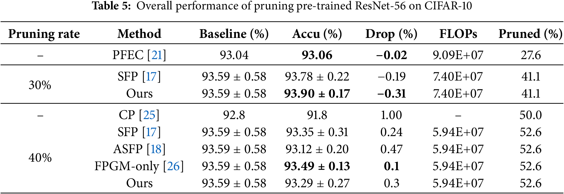
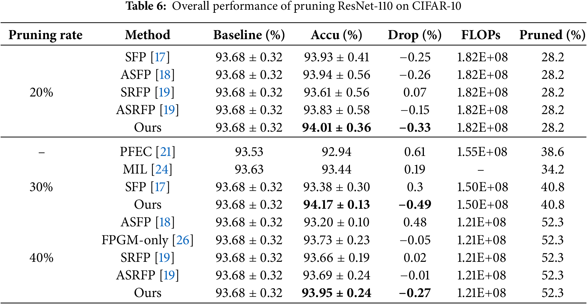
ResNet on CIFAR-10. Tables 2 to 7 present the experimental results for various network model structures and different pruning rates with our algorithm on the CIFAR-10 dataset. These tables compare our method against other pruning algorithms, with the results of competing methods taken from their respective papers. In the tables, “Ours” represents our algorithm, and the highest accuracy within each category is highlighted in bold. Table 2 shows the performance of ResNet-20 trained from scratch at different pruning rates, allowing us to observe how pruning impacts smaller network structures. Table 3 details the results for ResNet-32 trained from scratch with varying pruning rates, illustrating how the algorithm performs on slightly deeper networks. Table 4 displays the performance of ResNet-56 trained from scratch at different pruning rates, highlighting the effects of pruning on mid-sized networks. Table 5 focuses on a pre-trained ResNet-56, allowing for a comparison between training from scratch and pruning a pre-trained model. Table 6 provides data on ResNet-110 trained from scratch with different pruning rates, emphasizing how pruning impacts deeper networks. Table 7 shows the performance of a pre-trained ResNet-110, demonstrating how our algorithm enhances accuracy even with pre-trained models.

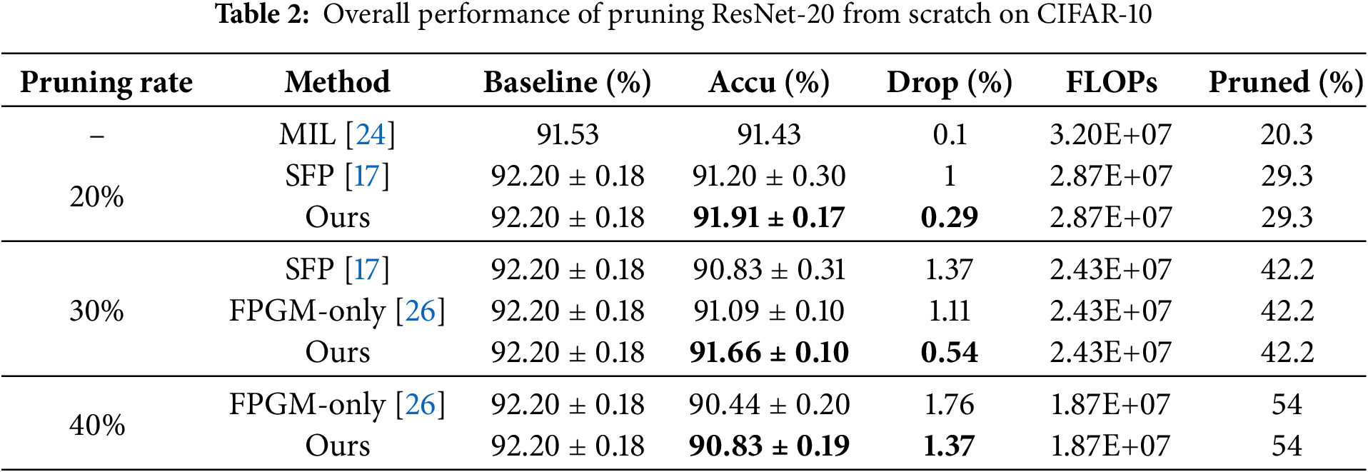
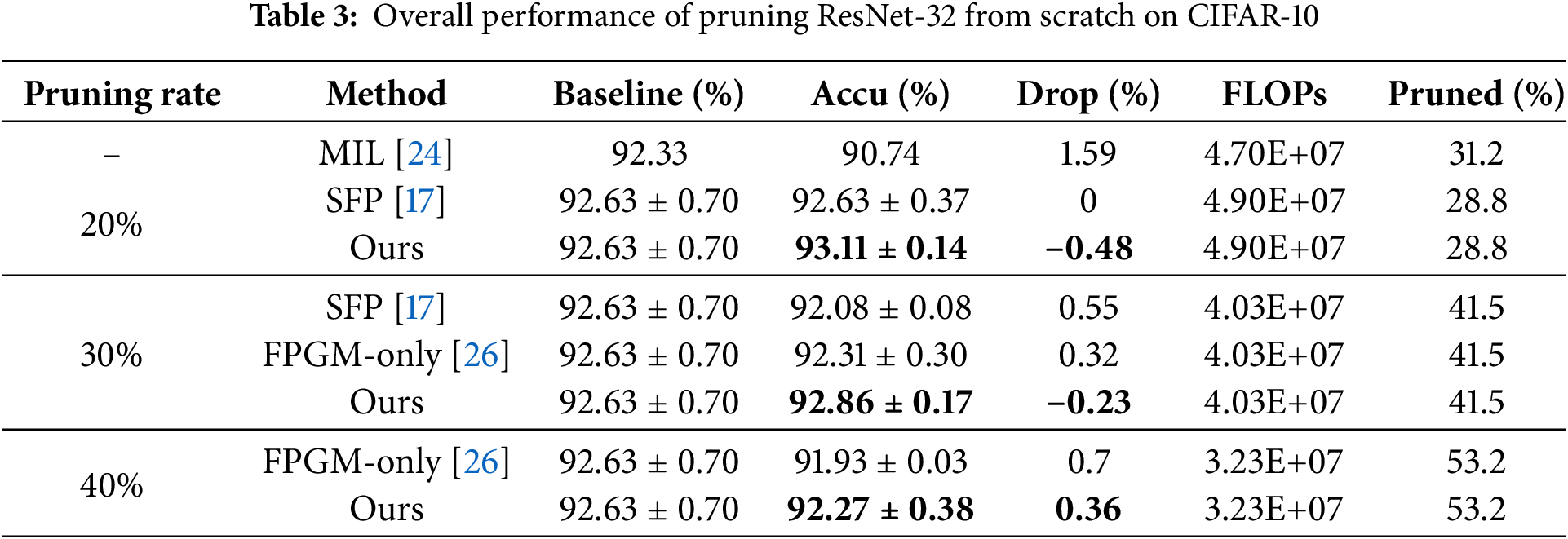
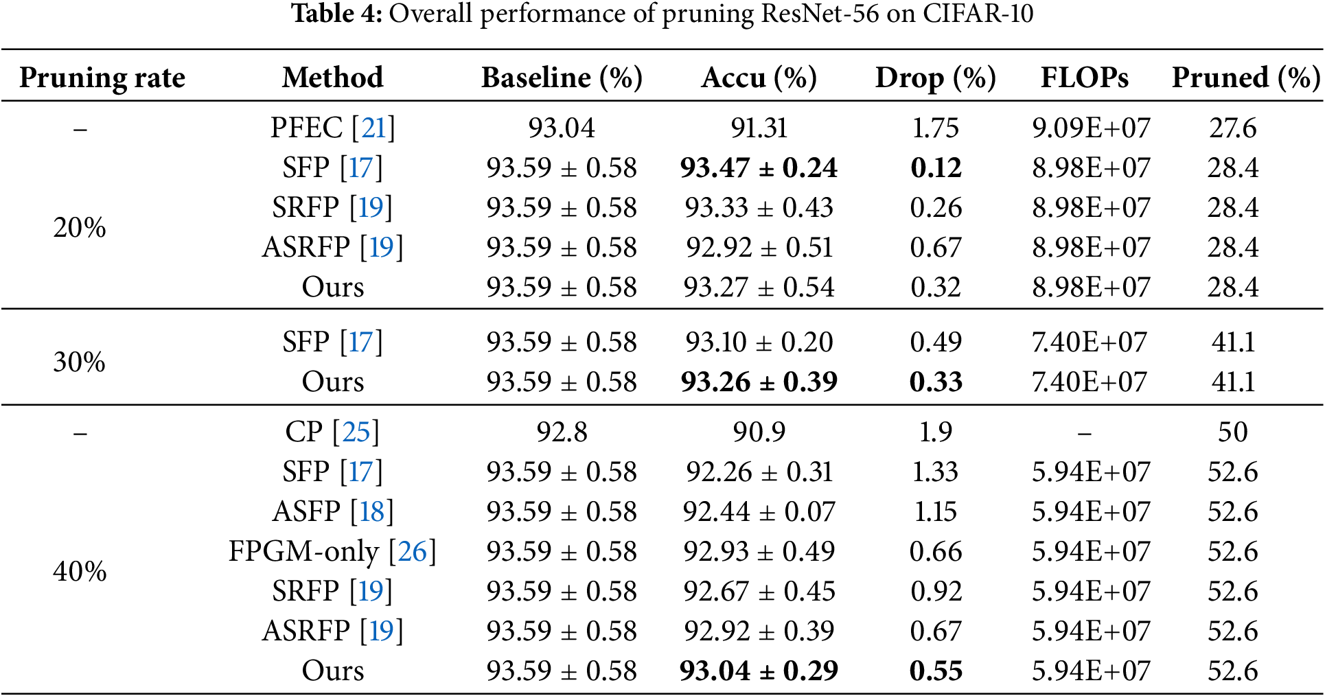
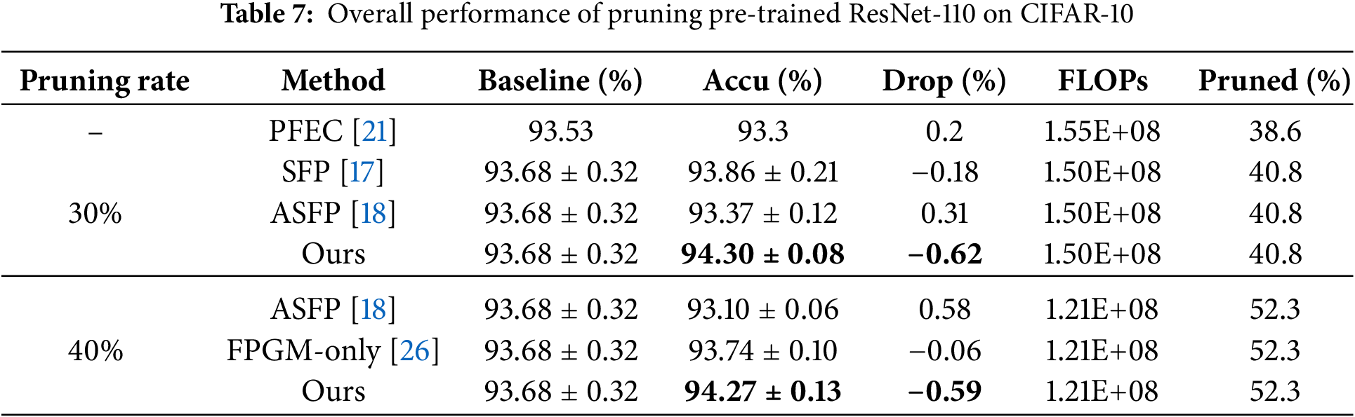
From Tables 2 to 7, we can see that our algorithm generally outperforms other algorithms in accuracy. In comparison with hard pruning algorithms MIL [24], PFEC [21], and CP [25], it is essential to refer to the “Drop” column data for a rough comparison with our algorithm, as the decrease ratio of floating-point numbers varies among algorithms.

The proposed algorithm performs exceptionally well on the ResNet-110 architecture. For different pruning rates, the accuracy consistently surpasses SFP [17] and other flexible pruning algorithms. Moreover, the network’s accuracy improves after pruning with our algorithm compared to the original network. Specifically, with a pruning rate of 30% for ResNet-110, the pruned network not only decreases the floating-point calculation by 40.8% but also enhances the classification accuracy by 0.49%. The accuracy improvement is even more significant on the pre-trained ResNet-110 network, reaching 0.62%. This indicates that our algorithm demonstrates outstanding performance on deeper networks.

Our algorithm consistently achieves optimal results for the shallow network models, ResNet-20 and ResNet-32.

ResNet on ILSVRC-2012. The experiments on the ILSVRC-2012 dataset are generally similar to those on the CIFAR-10 dataset, but we focus on comparing our algorithm with other flexible pruning algorithms. The relevant experimental results are presented in Tables 8 and 9.

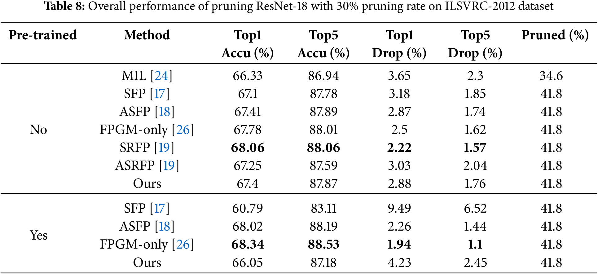
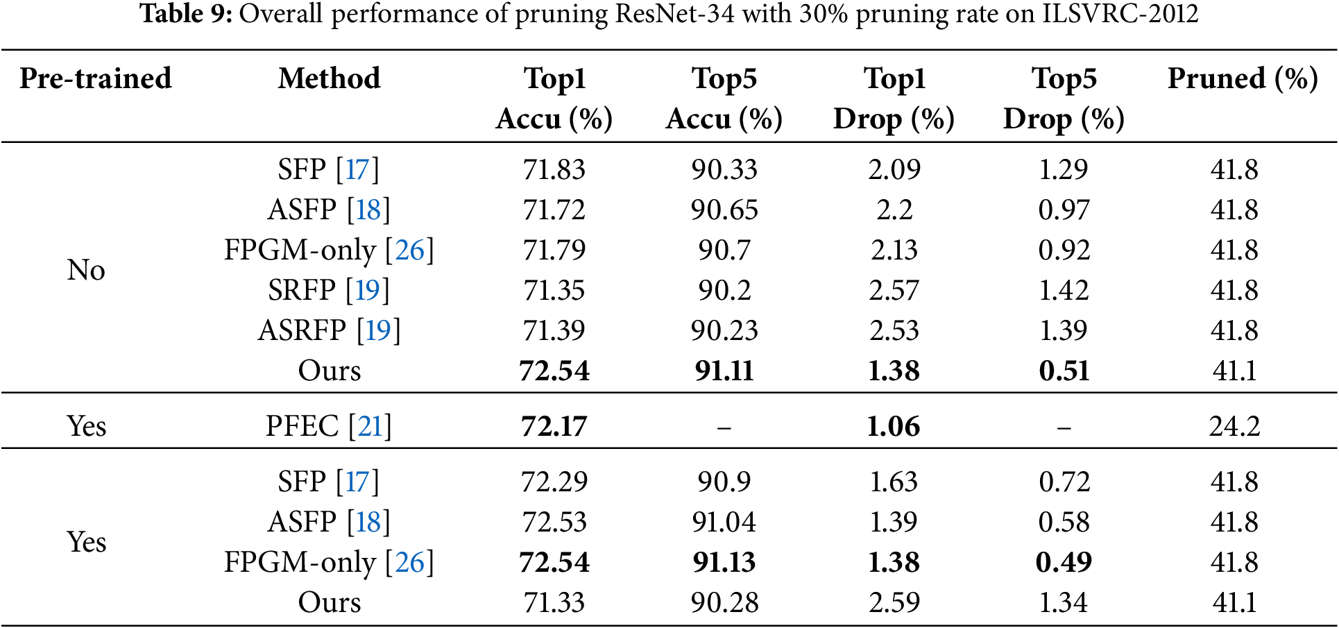
Table 9 shows that on the ResNet-34 architecture, with a pruning rate of 30%, our algorithm achieves a Top1 accuracy of 72.54% and Top5 accuracy of 91.11%. This compares favourably to the original network, which only experiences a decrease of 1.38% in Top1 accuracy and 0.51% in Top5 accuracy after pruning. Notably, our algorithm outperforms the experimental results of the SFP [17] algorithm and exhibits superior performance compared to other flexible pruning algorithms. This indicates that our algorithm can be used well for different complex datasets.

4.2 Ablation Study

To validate the effectiveness of various modules and parameters in the proposed algorithm, we conducted relevant ablation experiments to investigate the impact of pruning rate, hyperparameter C, hyperparameter , and the adaptive attenuation module on the pruning performance.

Different Pruning Rates. Our algorithm was applied with various pruning rates to ResNet-56 and ResNet-110, and the impact of these pruning rates on accuracy is shown in Fig. 5. For ResNet-56, although the accuracy of the pruned network is lower than that of the original network, the decrease is insignificant, and the pruned network still performs adequately. In contrast, for ResNet-110, when the pruning rate is set to 40%, the pruned network achieves an accuracy that surpasses that of the original network. This suggests that, at this pruning rate, the network’s most important filters are retained, and pruning does not hinder its performance.

Figure 5: The impact of pruning rate on accuracy

Comparing the accuracy trends for both networks, a clear negative correlation between pruning rates and accuracy can be observed. Specifically, when the pruning rate is below 60%, the accuracy drop remains relatively small, around 2%. However, once the pruning rate exceeds 60%, the accuracy begins to decline more sharply. This phenomenon implies that a large portion of the filters contributes minimally to the network’s performance, with the most significant feature information being encoded in the remaining 40% of filters. These findings indicate that our algorithm effectively reduces the network’s parameter count without significantly compromising performance.

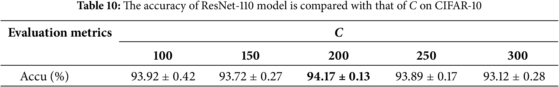
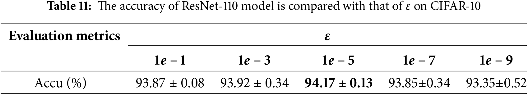
Hyperparameters C and . Our algorithm includes two important hyperparameters: C and . To determine their optimal values, experiments were conducted using ResNet-110 with a 30% pruning rate on the CIFAR-10 dataset. Five different values for C were tested: 100, 150, 200, 250, and 300, with results shown in Table 10. These results show that setting C to 200 yields the best classification accuracy, providing the optimal balance between pruning and network performance. The hyperparameter was also tested, with the results in Table 11. When was set to , the network achieved the best performance, suggesting that this value of provides the best trade-off between pruning rate and accuracy retention.

Adaptive Attenuation Module. This section assesses the effectiveness of the adaptive attenuation module by comparing the results with and without its removal. We conducted experiments on ResNet-56 and ResNet-110 networks using pruning rates of 20%, 30%, and 40%, both with and without the adaptive attenuation module. As shown in Fig. 6, except for the case where ResNet-56 has a pruning rate of 20%, where the algorithm in this paper outperforms others, the advantages of the proposed method are visible in the other scenarios. Specifically, the adaptive attenuation module significantly enhances pruning accuracy and model stability, highlighting its importance in the pruning process.

Figure 6: Comparison with and without adaptive module

5  Conclusions

In this study, we proposed a soft pruning algorithm based on the solution to the Logistic Growth Differential Equation to provide more precise control over the neural network pruning process. The algorithm dynamically adjusts the decay rate throughout the training process, taking advantage of the characteristics of the logistic growth curve. By incorporating the L2 norm of the filter weights into the decay rate calculation, an adaptive mechanism was introduced to refine pruning decisions and minimize unnecessary information loss. Our approach effectively manages the pruning process, maintaining model performance while reducing computational load.

When compared to existing progressive soft pruning methods, such as SFP, ASFP [18], and ASRFP [19], our algorithm demonstrates comparable or superior classification accuracy and prediction stability on the CIFAR-10 and ILSVRC-2012 datasets. These results highlight the potential of our algorithm for network optimization, offering a robust and flexible approach for pruning deep neural networks.

However, certain limitations should be acknowledged to improve the applicability of the proposed method further. First, the algorithm’s performance is sensitive to the choice of pruning rate. While it has shown promising results at pruning rates up to 40%, excessively high pruning rates may lead to a loss of essential information, which could degrade the model’s accuracy. Thus, adaptive pruning strategies that dynamically adjust pruning rates based on performance feedback would be a useful direction for future work.

Second, the proposed algorithm primarily focuses on convolutional neural networks (CNNs) like ResNet, and its effectiveness on other types of architectures, such as recurrent neural networks (RNNs) or transformer models, has not been thoroughly explored. Extending the method to more diverse architectures will be crucial to assess its generalizability across different neural network types.

Third, introducing the logistic growth differential equation for weight attenuation adds slight computational overhead, particularly in the early stages of training. While this overhead is relatively small compared to the overall training time, it may still be a concern in resource-constrained environments or when working with large models.

Lastly, although the use of L2 norm-based adaptive pruning helps preserve important weights, it may still lead to the inadvertent pruning of small but crucial weights in certain network structures. Careful control of pruning thresholds or incorporating additional heuristics for important filters could mitigate this issue.

In future work, we plan to address these limitations by exploring more flexible pruning rate strategies, testing the algorithm on a broader range of architectures, and investigating methods to reduce the computational cost of weight attenuation. Additionally, applying the pruning algorithm to more complex vision tasks, such as object detection, semantic segmentation, and image synthesis, will further demonstrate its effectiveness in real-world applications.

Acknowledgement: We appreciate the anonymous reviewers for their valuable feedback. Additionally, we extend our heartfelt gratitude to our families and friends for their unwavering support and encouragement.

Funding Statement: This work is partially supported by the National Natural Science Foundation of China under Grant No. 62172132.

Author Contributions: Can Hu: Conceptualization, Methodology, Software, Validation, Writing—original draft, Writing—review & editing, Visualization. Shanqing Zhang: Conceptualization, Methodology, Supervision, Project administration, Validation, Writing—review & editing. Kewei Tao: Writing—review & editing, Visualization. Gaoming Yang: Conceptualization, Methodology, Software, Validation, Conceptualization, Methodology, Resources, Writing—original draft, Writing—review & editing, Visualization. Li Li: Project administration, Funding acquisition, Validation, Software, Resources, Writing—review editing, Visualization. All authors reviewed the results and approved the final version of the manuscript.

Availability of Data and Materials: The data were prepared and analyzed in this study and are available upon request to the corresponding author.

Ethics Approval:: Not applicable.

Conflicts of Interest: The authors declare no conflicts of interest to report regarding the present study.

References

1. LeCun Y, Bengio Y. Convolutional networks for images, speech, and time series. In: The handbook of brain theory and neural networks. USA: MIT Press; 1995. [Google Scholar]

2. Girshick R. Fast R-CNN. In: Proceedings of the IEEE International Conference on Computer Vision; 2015. p. 1440–8. doi:10.1109/iccv.2015.169. [Google Scholar] [CrossRef]

3. Jia D, Yuan Y, He H, Wu X, Yu H, Lin W, et al. DETRs with hybrid matching. In: Proceedings of the IEEE/CVF Conference on Computer Vision and Pattern Recognition; 2023. p. 19702–12. doi:10.1109/cvpr52729.2023.01887. [Google Scholar] [CrossRef]

4. He K, Zhang X, Ren S, Sun J. Deep residual learning for image recognition. In: Proceedings of the IEEE Conference on Computer Vision and Pattern Recognition; 2016. p. 770–8. doi:10.1109/cvpr.2016.90. [Google Scholar] [CrossRef]

5. Simonyan K, Zisserman A. Very deep convolutional networks for large-scale image recognition. arXiv:1409.1556. 2014. [Google Scholar]

6. Krizhevsky A, Sutskever I, Hinton GE. Imagenet classification with deep convolutional neural networks. In: Advances in neural information processing systems. Association for Computing Machinery; 2012. Vol. 25. doi:10.1145/3065386. [Google Scholar] [CrossRef]

7. Chen W, Si C, Zhang Z, Wang L, Wang Z, Tan T. Semantic prompt for few-shot image recognition. In: Proceedings of the IEEE/CVF Conference on Computer Vision and Pattern Recognition; 2023. p. 23581–91. doi:10.48550/arXiv.2303.14123. [Google Scholar] [CrossRef]

8. Noh H, Hong S, Han B. Learning deconvolution network for semantic segmentation. In: Proceedings of the IEEE International Conference on Computer Vision; 2015. p. 1520–8. doi:10.1109/iccv.2015.178. [Google Scholar] [CrossRef]

9. Ru L, Zheng H, Zhan Y, Du B. Token contrast for weakly-supervised semantic segmentation. In: Proceedings of the IEEE/CVF Conference on Computer Vision and Pattern Recognition; 2023. p. 3093–102. doi:10.1109/cvpr52729.2023.00302. [Google Scholar] [CrossRef]

10. Szegedy C, Vanhoucke V, Ioffe S, Shlens J, Wojna Z. Rethinking the inception architecture for computer vision. In: Proceedings of the IEEE Conference on Computer Vision and Pattern Recognition; 2016. p. 2818–26. doi:10.1109/cvpr.2016.308. [Google Scholar] [CrossRef]

11. Sandler M, Howard A, Zhu M, Zhmoginov A, Chen L-C. MobileNetv2: inverted residuals and linear bottlenecks. In: Proceedings of the IEEE Conference on Computer Vision and Pattern Recognition; 2018. p. 4510–20. doi:10.1109/CVPR.2018.00474. [Google Scholar] [CrossRef]

12. Gholami A, Kim S, Dong Z, Yao Z, Mahoney MW, Keutzer K. A survey of quantization methods for efficient neural network inference. In: Low-power computer vision. USA: Chapman and Hall/CRC; 2022. p. 291–326. [Google Scholar]

13. Hinton G, Vinyals O, Dean J. Distilling the knowledge in a neural network. arXiv:1503.02531, 2015. [Google Scholar]

14. Pei R, Liu J, Li W, Shao B, Xu S, Dai P, et al. CLIPPING: distilling clip-based models with a student base for video-language retrieval. In: Proceedings of the IEEE/CVF Conference on Computer Vision and Pattern Recognition; 2023. p. 18983–92. doi:10.1109/CVPR52729.2023.01820. [Google Scholar] [CrossRef]

15. Davoodi P, Gwon C, Lai G, Morris T. Tensorrt inference with tensorflow. GPU Technology Conference; 2019 [cited 2024 Jan 21]. Available from: https://developer.download.nvidia.com/video/gputechconf/gtc/2019/presentation/s9431-tensorrt-inference-with-tensorflow.pdf. [Google Scholar]

16. Studio A. Neural networks api | android ndk [cited 2024 Jan 21]. 2024. Available from: https://developer.android.com/ndk/guides/neuralnetworks?hl=zh-cn. [Google Scholar]

17. He Y, Kang G, Dong X, Fu Y, Yang Y. Soft filter pruning for accelerating deep convolutional neural networks. arXiv:1808.06866. 2018. [Google Scholar]

18. He Y, Dong X, Kang G, Fu Y, Yan C, Yang Y. Asymptotic soft filter pruning for deep convolutional neural networks. IEEE Trans Cybern. 2019;50(8):3594–604. doi:10.1109/TCYB.2019.2933477. [Google Scholar] [PubMed] [CrossRef]

19. Cai L, An Z, Yang C, Xu Y. Softer pruning, incremental regularization. In: 2020 25th International Conference on Pattern Recognition (ICPR). 2021. p. 224–30. doi:10.1109/ICPR48806.2021.9412993. [Google Scholar] [CrossRef]

20. Fang G, Ma X, Song M, Mi MB, Wang X. Dep Graph: towards any structural pruning. In: Proceedings of the IEEE/CVF Conference on Computer Vision and Pattern Recognition; 2023. p. 16091–101. doi:10.1109/CVPR52729.2023.01544. [Google Scholar] [CrossRef]

21. Li H, Kadav A, Durdanovic I, Samet H, Graf HP. Pruning filters for efficient convnets. arXiv:1608.08710. 2016. [Google Scholar]

22. Krizhevsky A, Hinton G. Learning multiple layers of features from tiny images. 2009 [cited 2024 Jan 21]. Available from: https://www.cs.utoronto.ca/~kriz/learning-features-2009-TR.pdf. [Google Scholar]

23. Russakovsky O, Deng J, Su H, Krause J, Satheesh S, Ma S, et al. ImageNet large scale visual recognition challenge. Int J Comput Vis. 2015;115(3):211–52. doi:10.1007/s11263-015-0816-y. [Google Scholar] [CrossRef]

24. Dong X, Huang J, Yang Y, Yan S. More is less: a more complicated network with less inference complexity. In: Proceedings of the IEEE Conference on Computer Vision and Pattern Recognition; 2017. p. 5840–8. doi:10.1109/CVPR.2017.205. [Google Scholar] [CrossRef]

25. He Y, Zhang X, Sun J. Channel pruning for accelerating very deep neural networks. In: Proceedings of the IEEE International Conference on Computer Vision; 2017. p. 1389–97. doi:10.1109/ICCV.2017.155. [Google Scholar] [CrossRef]

26. He Y, Liu P, Wang Z, Hu Z, Yang Y. Filter pruning via geometric median for deep convolutional neural networks acceleration. In: Proceedings of the IEEE/CVF Conference on Computer Vision and Pattern Recognition; 2019. p. 4340–9. doi:10.1109/CVPR.2019.00447. [Google Scholar] [CrossRef]