Deep Convolution Neural Networks for Image-Based Android Malware Classification

1  Introduction

Malware poses significant threats to individuals, businesses, and the global economy as technology evolves rapidly [1,2]. Due to the versatility of new malware, traditional signature-based detection methods are inadequate. Thus, exploring innovative detection techniques is essential. Deep convolutional neural networks (CNNs) have shown promise in enhancing malware detection systems through image processing [3].

Malware, defined as malicious software, exploits computer vulnerabilities and can lead to data theft and process disruptions [4]. With over ten billion attacks annually, improving detection and prevention is urgent, as evidenced by rising malware incidents from 2022 to 2023 [4,5]. CNNs are commonly used to analyze visual features of malware [6,7]. Ensemble methods like voting and stacking have proven effective for detecting Android malware [8,9], achieving up to 90.4% performance scores. Advanced frameworks, such as “FalDroid,” have reached 94% accuracy in Android malware detection [10]. New tools like Marvin utilize machine learning alongside static and dynamic analysis, achieving a high accuracy of 98.24% on large datasets [11]. Techniques combining ontology and reverse engineering with SPARQL have also demonstrated effectiveness in early malware identification [12]. The VGG16 model, with its 16 layers, excels in categorizing Android malware using images, preventing overfitting and enhancing model generalization [13,14].

Fig. 1 illustrates the proposed malware detection architecture, which employs pre-trained DCNN model, followed by updated VGG16 layers and image fine-tuning techniques for improved performance in recognizing intricate malware patterns.

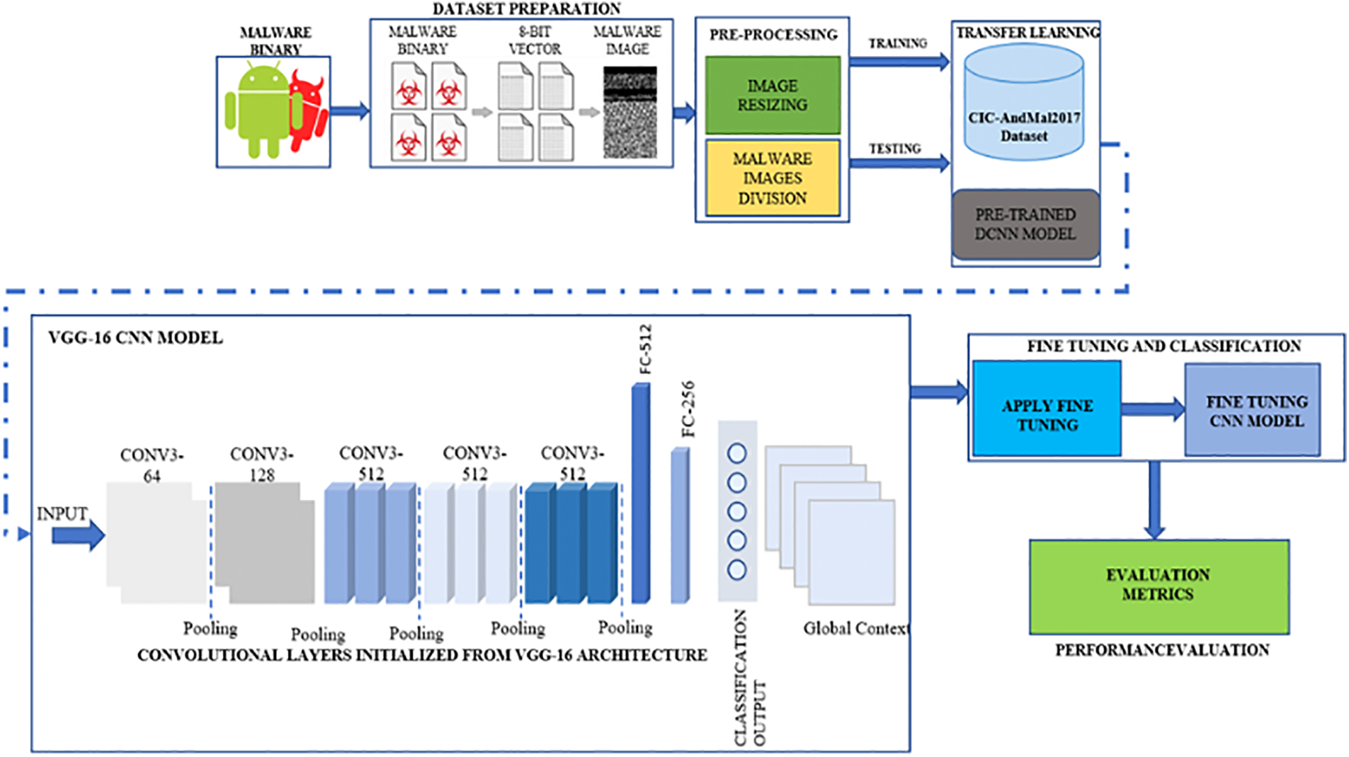
Figure 1: A deep convolutional neural network and image processing framework for malware detection

The contributions of the research paper are as follows:

1.   Novel Malware Detection Method: Introduces a new approach using image processing, Deep Convolutional Neural Networks (DCNN), and updated VGG16, moving beyond traditional signature-based and behavior-based methods.

2.   Enhanced Classification Accuracy: Demonstrates that using images of malware samples improves differentiation between malware types.

3.   Impact on Cybersecurity: The results strengthen existing anti-malware solutions, improving network protection against advanced threats.

4.   Foundation for Future Research: The study paves the way for further innovation in malware detection techniques.

The following is a breakdown of this study’s structure: Section 2 will present the literature review, and Section 3 will describe the datasets. Section 4 will describe the methodologies, also referred to as the approach. Section 5 will involve the experiment, while Section 6 will analyze the experiment’s results. Finally, Section 7 will conclude the entire study.

2  Literature Review

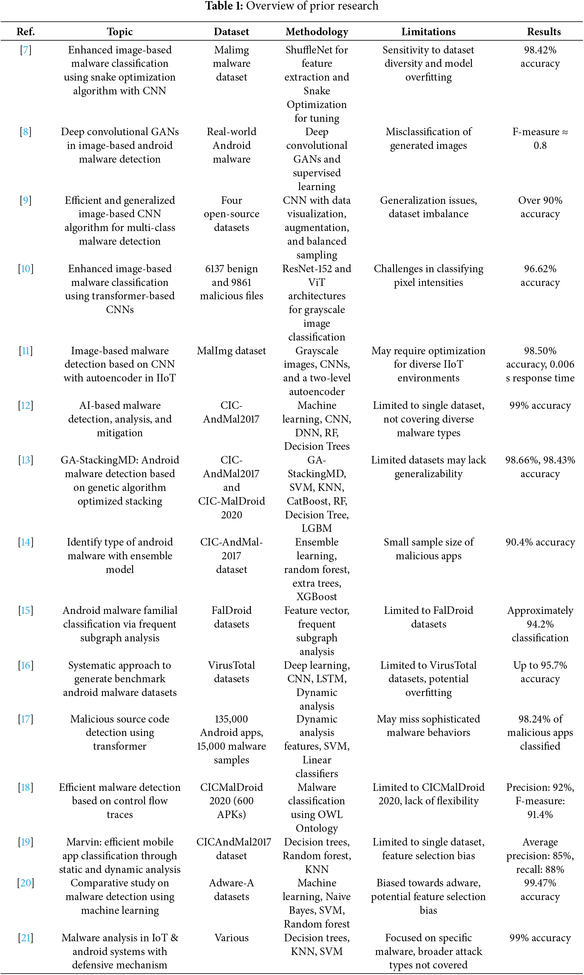
This section examines recent research on the classification of Android malware using deep learning, analyzing methodologies, datasets, results, and limitations to evaluate whether our proposed method addresses existing challenges.

Current research in image-based malware classification has focused on using deep learning approaches to improve accuracy. Duraibi et al. [7] proposed a hybrid approach combining the Snake Optimization algorithm with a deep CNN for feature extraction via ShuffleNet, achieving an accuracy of 98.42% on the Malimg dataset. Still, they noted potential issues with model overfitting and dataset sensitivity. Similarly, Mercaldo et al. [8] explored deep convolutional GANs for distinguishing real from fake malware images, reporting an F-measure close to 0.8, but identified misclassification of some generated images as a significant flaw. Liu et al. [9] addressed challenges related to poor algorithm generalization and imbalanced datasets by employing a CNN architecture alongside data visualization, augmentation, and balanced sampling, achieving an accuracy of 91.48%. Ashawa et al. [10] extended the Transformer-based CNN approach, achieving 99.62% accuracy with grayscale malware images, although they acknowledged computational drawbacks in pixel intensity classification. Kumar et al. [11] utilized an autoencoder with CNNs, attaining 98.50% accuracy, demonstrating the efficiency of image-based malware detection across various conditions. Djenna et al. [12] examined malware detection using the CIC-AndMal2017 dataset, achieving 99% accuracy with CNNs, but their reliance on a single dataset raises concerns about generalization and overfitting. Xie et al. [13] introduced the GA-StackingMD method, achieving accuracies of 98.66% and 98.43% on two datasets, though their analysis was based on small datasets, which may introduce bias. Arslan et al. [14] also used the CIC-AndMal2017 dataset, achieving 90.4% accuracy with ensemble learning techniques, but the limited number of malicious samples raises questions about real-world applicability. Fan et al. [15] focused on the family classification of Android malware, achieving a classification rate of approximately 94.2%, but their reliance on a specific dataset limits generalization. Lashkari et al. [16] proposed a static and dynamic analysis approach using VirusTotal datasets, achieving accuracy between 93.0% and 95.7% with CNN and LSTM networks. Still, their dynamic analysis method raises concerns regarding its effectiveness against diverse malware variants. Tsfaty et al. [17] investigated malicious source code detection using dynamic analysis, achieving 98.24% accuracy, but noted limitations in identifying complex malware behaviors. Qiang et al. [18] classified malware based on control flow using deep neural networks, achieving 92% precision and 91.4% F-measure, but their ontology-based classification may struggle with newer malware variants. Lindorfer et al. [19] achieved 85% precision and 88% recall using static and dynamic analysis, but feature selection biases limited their findings. Pavithra et al. [20] conducted a comparative analysis using the Adware-A dataset, finding that Random Forest outperformed Naive Bayes and SVM with an accuracy of 99.47%. Still, their focus on adware raises questions about applicability to other malware types. Lastly, Yadav et al. [21] discussed malware incidents in IoT and Android systems, achieving 99% accuracy using decision trees, KNN, and SVM, but noted that some types of malicious programs remain underexplored.

The reviewed studies demonstrate significant advancements in deep learning and machine learning for Android malware classification. However, common limitations include small and non-diverse datasets, potential overfitting, and selection bias. Many current approaches rely on specific datasets that do not adequately reflect emerging Android malware, limiting their real-world applicability. Our proposed method addresses these challenges by utilizing a more extensive and diverse dataset, optimizing deep convolutional networks for image-based data, and implementing regularization techniques to mitigate overfitting. This comprehensive approach positions our contribution as a robust and flexible solution to the evolving challenges of Android malware classification, paving the way for further research in malware detection technologies.

Table 1 lists prior papers cited with datasets, methods, limitations, and results. This table serves as a concise reference for understanding the landscape of Android malware classification studies, highlighting their contributions and shortcomings.

3  Data Collection

The data for this study was obtained from the Android Malware Dataset (CIC-AndMal2017) [13,15,16], maintained by the Canadian Institute for Cybersecurity. Available in APKS, CSVS, and PCAPS formats, the investigation focused on a CSV dataset containing zip files with various types of malwares, including adware, ransomware, scareware, and SMS malware. The study processed these files to create a larger dataset encompassing all classes and their respective sample sizes, ensuring a suitable class distribution.

The CIC-AndMal2017 dataset consists of 20,000 instances of network traffic data derived from various Android malware types, categorized into five classes: Trojan, Adware, Ransomware, Spyware, and Worm. Each instance has 84 features, including source and destination IP addresses, ports, protocols, flow duration, and packet counts. This data was collected through controlled experiments simulating realistic malware activity, providing a solid foundation for malware detection.

Visualizing the distribution and features of each class is crucial for understanding their impact on the training and testing processes of machine learning algorithms. Different malware classes exhibit distinct traffic patterns, influencing detection rates and speeds. We can enhance their models by analyzing these differences for more effective threat identification and mitigation. Additionally, understanding how class characteristics affect model performance will aid in developing advanced detection mechanisms, thereby improving cybersecurity against various malware threats.

Table 2 categorizes the occurrences into five distinct forms of malware attacks. The target variable serves as the class label for these forms.

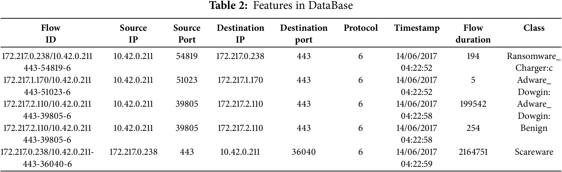
•   Ransomware_Charger: Malware samples in this category display ransomware behavior, generally encrypting the victim’s data and demanding a ransom to unlock it.

•   Adware_Dowgin: Malware samples in this category are mostly adware, which displays invasive advertising for the attackers to gain cash.

•   Scareware_Androiddefender: Scareware malware fraudulently promises security protection to trick users into purchasing bogus antivirus software.

•   Smsmalware_Fakeinst: This category of malware focuses on SMS-related attacks. It is frequently camouflaged as genuine programs while surreptitiously sending unauthorized premium-rate text messages.

•   Benign: This class describes harmless network traffic or lawful programs that do not behave maliciously.

The dataset provides a comprehensive representation of Android malware attacks, facilitating the development and evaluation of robust machine-learning algorithms for accurate categorization and detection. Understanding its characteristics, feature distributions, and class imbalances is essential for effective data preparation, feature engineering, and model training. Analyzing and visualizing this information offers valuable insights into Android malware features, helping to enhance machine-learning solutions in cybersecurity.

3.1 Exploratory Data Analysis

Exploratory data analysis (EDA) techniques were employed on the Android malware dataset to gain insights into its intrinsic characteristics [22]. EDA is crucial for identifying patterns, trends, outliers, and potential issues within a dataset, guiding subsequent data preparation and modeling steps. Key findings from the EDA include:

•   Label Distribution: This section analyses the distribution of labels among Android malware categories, visualized through a bar plot. This analysis reveals essential insights into the frequency of malware attacks in the dataset [23]. The x-axis represents distinct malware types, while the y-axis indicates incident frequency. Fig. 2 illustrates the distribution of different malware categories.

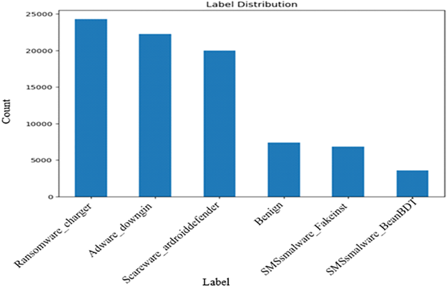
Figure 2: Malware class distribution

The figure presents the label distribution within the Android malware dataset. Ransomware-charger has the highest frequency of around 21,000 instances, followed by Adware-downing at 19,000 and Scareware-android Defender at 17,500. Benign samples account for approximately 10,000 instances, while the remaining labels have significantly lower frequencies, ranging from 1000 to 5000. This imbalanced distribution is an essential consideration for data preparation, feature engineering, and model training, potentially requiring techniques like oversampling, under-sampling, or class weighting to ensure the model learns effectively and generalizes well across different malware types [24,25].

i. Exploring Relationships among Selected Android Malware Variables

Fig. 3 illustrates the relationships among selected variables in the Android malware dataset, focusing on total forward packets, total backward packets, forward packet lengths, and malware labels. The heatmap utilizes a color scale to indicate correlation magnitude and direction, with warmer colors representing positive correlations and cooler colors indicating negative correlations. By exploring the heatmap, we can identify key variable dependencies that inform the development of effective malware detection and classification models. This visualization elucidates how these variables influence malware labels, facilitating the detection of significant features and underlying correlations within the dataset.

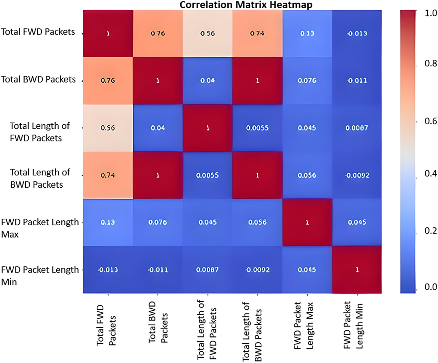
Figure 3: Correlation Matrix heatmap of selected features

In this analysis, we used a cut-off of 0.31 for feature selection, as previous research data suggested that coefficients more significant than this are significantly meaningful about the target variable. This value was set to reduce the model’s noise and accomplish the desired level of learning effectiveness. By extracting features with meaningful correlation, we intended to bring the dataset closer to being clean, where only related features are included, which can benefit the model.

However, it would be useful to reveal more detailed information about how this threshold influences performance measures that were previously discussed, including accuracy, precision, and recall rates. Knowledge of these dependencies may help explain the link between the chosen characteristics and the model’s efficiency [26,27]. From the results obtained from our analysis, it is highly likely that when the ideal set of features is used, better results, as compared to other possible combinations within the online sales dataset, are achieved. This evidence illustrates why feature selection is a critical consideration in developing reliable predictive models and proves that the selected correlation threshold in this study results in improved model performance.

The Correlation Matrix Heatmap in Fig. 3 provides valuable insights into the relationships between the selected variables in the Android malware dataset. The key insights are:

1.   Total Forward Packets and Total Backward Packets exhibit a strong positive correlation, indicated by the dark red hue in the corresponding cell of the heatmap. This suggests a close relationship between the number of packets sent in the forward and backward directions.

2.   The total lengths of forward and backward packets also show a positive correlation, though not as strong as the packet counts. This implies that the packet length characteristics are linked between the forward and backward traffic.

3.   The forward packet length-related variables, such as Total Length of FP, Max Length of FP, and Min Length of FP, demonstrate high positive correlations among themselves, as indicated by the warm red colors in the respective cells.

4.   The malware label variable shows moderate to strong positive correlations with the packet-related variables, suggesting that these numerical features may be necessary for distinguishing between different malware types.

5.   The overall color patterns in the heatmap indicate that the selected variables are not entirely independent and exhibit various degrees of interdependence, which is critical information for feature engineering and model development.

ii. Exploring Numerical Variables in the Android Malware Dataset: Histogram Analysis

Android malware “histogram analysis” shows numerical variable frequency and distribution patterns. The variables under consideration are the total number of forward and backward packets and their lengths as well as maximum and minimum lengths. Histograms show the distribution of values within a variable, revealing data features like range, skewness, and trends. Bins can be limited to 20 balances to collect distribution data and prevent excessive binning.

Moreover, Fig. 4 subplots show numerical variable histograms. Variable values are on the x-axis, and frequency is on the y-axis. Histograms show distribution characteristics like peaks, troughs, and asymmetry. They also reveal outliers. Histogram analysis helps understand data distribution, which is essential for feature engineering, outlier detection, and data preparation. Histograms can be examined to improve classification models by exploring data changes such as logarithmic scaling or normalization. The visualization helps researchers identify key elements in deep convolutional neural networks and image processing for malware detection.

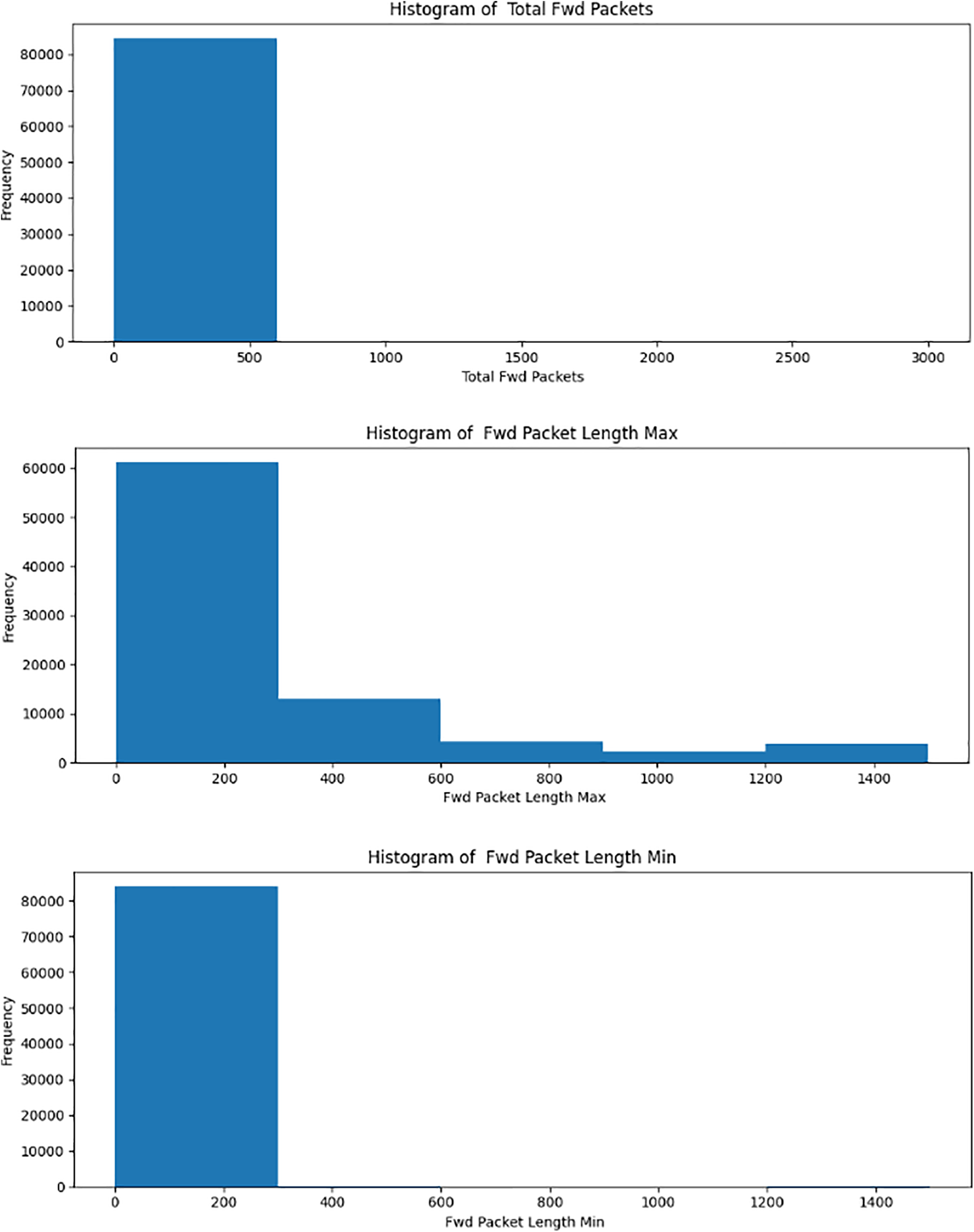
Figure 4: Numerical variables distribution of values

The above three figures show the distribution of feature variables, and we see that values are not continuous but rather more of a categorical nature as we have many classes in the dataset. It should be like there would be a range of these variables, each allocated to a particular class, but we see it remains more or less constant for a specific nature, which is also due to the reason that classes are imbalanced that’s why we are seeing this type of distribution and cannot label features directly to the class.

iii. Parallel Coordinates Plot of Selected Variables in the Android Malware Dataset

The “Parallel Coordinates Plot” shows Android malware dataset variables’ correlations and trends, as in Fig. 5. The variables under consideration are the total number of forward and backward packets and their lengths, as well as maximum and minimum lengths. The picture compares these parameters across malware classifications. Each line in the graphic represents a dataset sample, while the vertical axes reflect the selected variables [28,29]. Segments connect the lines, representing sample variable values. Assigning different colors or tints to each malware version label helps observe variation. The parallel coordinate plot can reveal patterns or trends in malware label variables. This helps determine each component’s relative importance and impact in distinguishing malicious software.

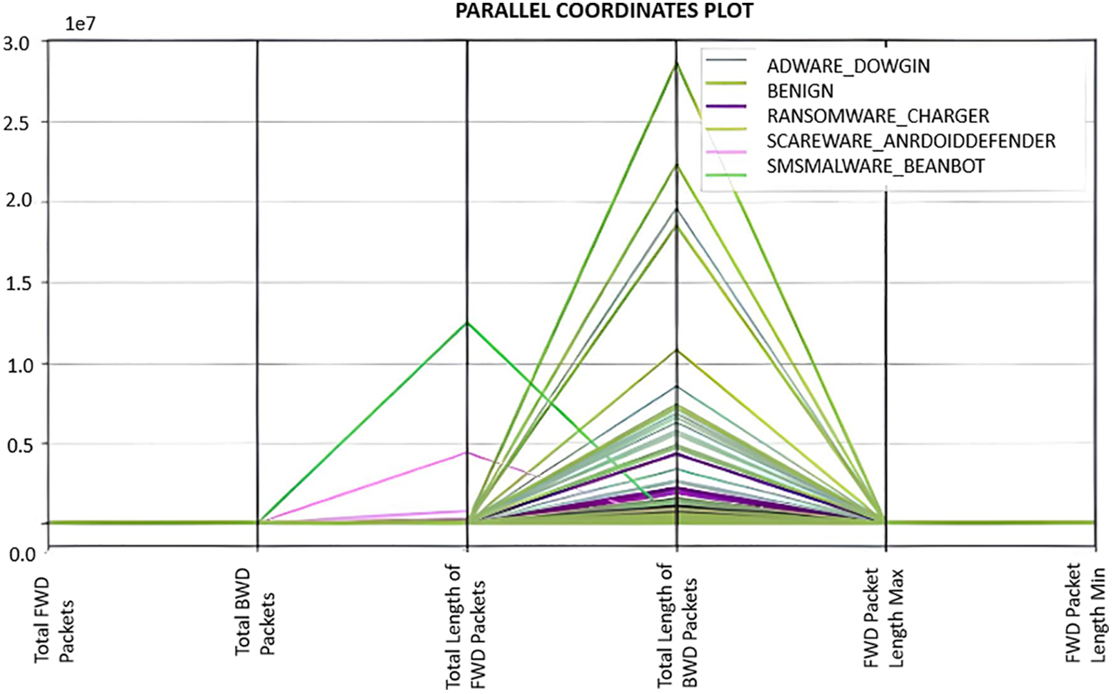
Figure 5: Parallel coordinates plot

Additionally, it may help identify virus categorization overlaps or similarities. The graphic helps researchers understand the associations between factors in the Android malware dataset. Parallel coordinate plots help identify malware-categorizing feature combinations. The knowledge is helpful in research on deep convolutional neural networks and image processing for malware detection.

These parallel coordinate plots basically show us how each data point in the features is associated with the label and other features. We can also see that each feature, for example, the total forward packet, is higher than the rest of the features, which is an indication of the key strength relationship of this feature with respect to the label.

iv. Radar Chart of Mean Values for Selected Variables in the Android Malware Dataset

Fig. 6 is a radar graphic showing the average values of Android malware dataset variables across types of malware. The graph examines the total forward, backward, total length, maximum length, and lowest length of forward packets. Further, this chart aims to compare mean variable values across malware types. Each chart axis depicts the mean value of a variable, with data points linked for each malware category to show mean value distribution. The radar map shows varying mean values among virus categories, revealing trends and key variables affecting malware categorization.

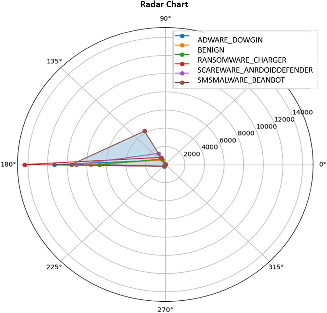
Figure 6: Radar chart of mean values for selected variables

This analysis shows how selected characteristics vary across viruses, revealing their properties. It also assists malware detection studies using deep convolutional neural networks and image processing by monitoring virus classification factor fluctuations.

It shows how selected features vary with the different classes we have. Suppose one class has more distribution of a particular feature. In that case, it will have a far-distant line, as we can notice in total forward packets, and those lines that are not far-distant will have less distribution of that particular feature. This plot helps us understand how each class is related to the features.

3.2 Data Preparation

The data processing steps for our study on Deep CNNs and Image Processing for Malware Detection are as follows:

     i)  Data Loading: We begin by loading the dataset, which includes malware samples and their properties, from multiple CSV files into a unified data frame using the Pandas library.

    ii)  Data Cleaning: Once the dataset is loaded, we clean it to address missing values, outliers, and anomalies, ensuring data quality and model effectiveness.

   iii)  Feature Selection: We focus on selecting essential features highlighting malware’s distinctive characteristics. Using correlation analysis and domain knowledge, we identify 64 significant features with a correlation coefficient of 0.31.

    iv)  Encoding of the Target Variable: We encode the target variable, which indicates the categories of malware (benign and four malicious actions), using label encoding. This process transforms categorical labels into numerical values for model training, representing a binary classification array [0, 1].

     v)  Splitting the Dataset: We split the dataset into training and testing sets, ensuring a consistent distribution of samples across malware categories. This approach facilitates malware classification while acknowledging the complexities of distinguishing between harmful and benign behaviours. The split Dataset size is as follows:

x_train x_test, y_train, y_test

(67434, 64) (16859, 64) (67434) (16859)

    vi)  Data Normalisation: We standardize the numerical attributes in the dataset to ensure consistent scaling and prevent any specific feature from overpowering the learning algorithm. Standardization is the technique employed in this case.

The diagram presented in Fig. 7 illustrates the sequence of steps involved in data preparation and the approach employed for categorizing malware.

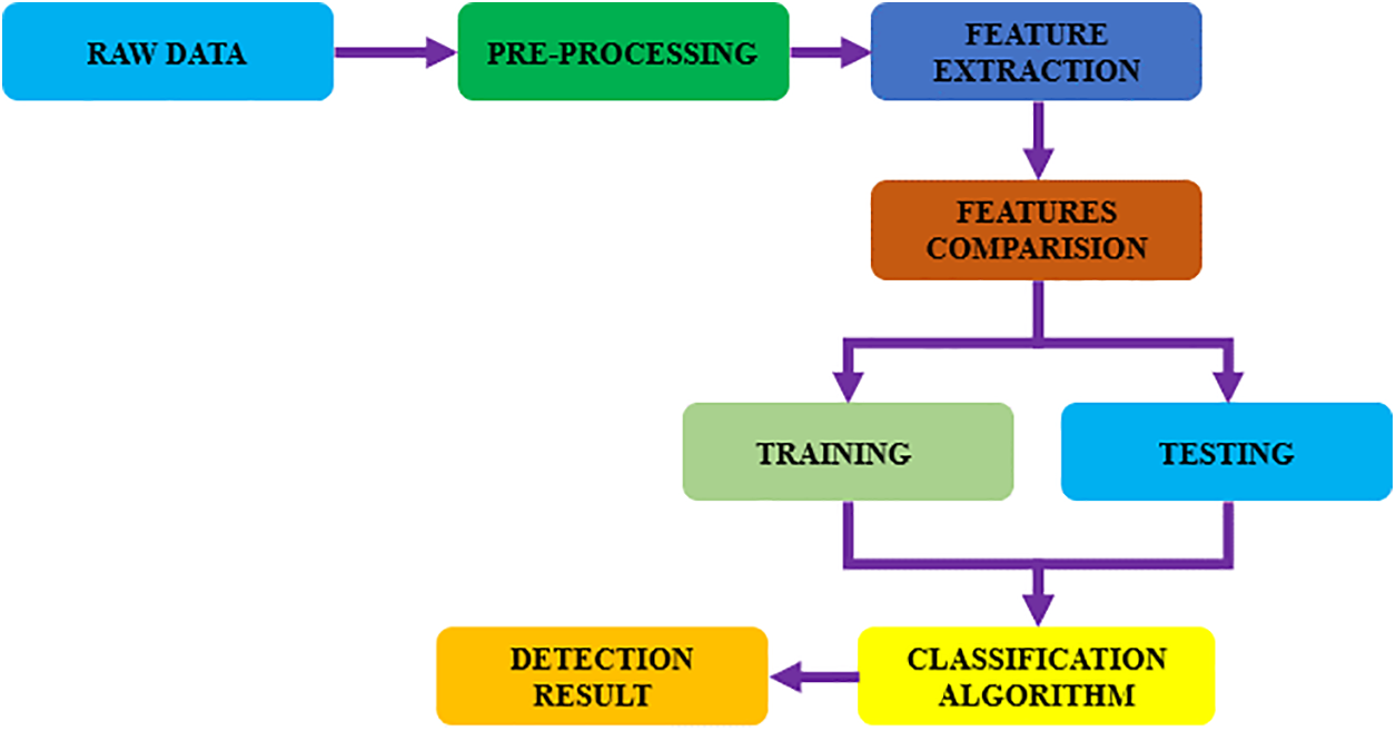
Figure 7: Data preparation methodology for malware classification

•   Image-Like Data Transformation: The 64-dimensional data becomes 32 × 32 × 3 by converting the data into image-like representations. Image processing reshapes the feature matrix into 2D or 3D arrays. CNN compatibility is accomplished by turning the dataset into a numpy array and transforming it into 32 × 8 × 8-pixel image-like representations. CNNs may successfully assess spatial relationships in data. Thus, while the original data samples had a dimension of 64, the modified data now fit the CNN analysis format (67434, 32, 32, 3) for the training set and (16859, 32, 32, 3) for the testing set.

•   Preparation for CNN Model: Preparing the data for the CNN model requires restructuring the features and labels into the appropriate structure and ensuring that the input shape is suitable for the selected CNN architecture, typically in 2D or 3D arrays.

•   Addressing Class Imbalance: Data balancing approaches are used if the dataset has a class imbalance, which means that particular malware classes are underrepresented. This could involve oversampling the minority class, undersampling the majority class, or generating synthetic data to achieve balance among the groups and avoid bias in the model.

Further, we employed oversampling techniques to address imbalanced classes to provide more instances of underrepresented classes to the model. In particular, the SMOTE algorithm was used for oversampling of the mentioned classes to create synthetic instances within the classes and enhance the variability of samples and, consequently, the model training. Moreover, we used different types of image augmentation, like rotation and flipping, to enhance the size of our image’s dataset. These transformations not only helped increase the volume of training data but also contributed to a better generalization capability of some of the transformations to variations in the representation of the malware. Thus, our major idea was to enhance the model’s capabilities to classify various types of malware by creating hallucinated views and orientations of the images.

Preparing and optimizing the dataset for training a deep CNN with mixed CNN layers for malware detection involves following specific data processing procedures. These procedures facilitate data cleaning, feature selection, normalization, and transformation, improving the model’s accuracy and reliability.

3.3 VGG16 CNN Model for Classification of Malware Attacks

The VGG16 model in Fig. 8 shows that CNN architectures are still effective image classifiers. Since its 2014 introduction for image recognition using the ImageNet dataset, it has expanded to include malware detection. The 16-layer, mostly convolutional model extracts hierarchical features from input images sequentially, capturing detailed patterns and features on various scales. The model accumulates higher-level features through convolutional and pooling layers and then classifies them through fully connected layers. Dropout regularization is used to reduce overfitting and improve generalization. The model matches the dimensions of the malware dataset by customizing the input shape and output layer neuron count and optimizes classification accuracy using modified stochastic gradient descent.

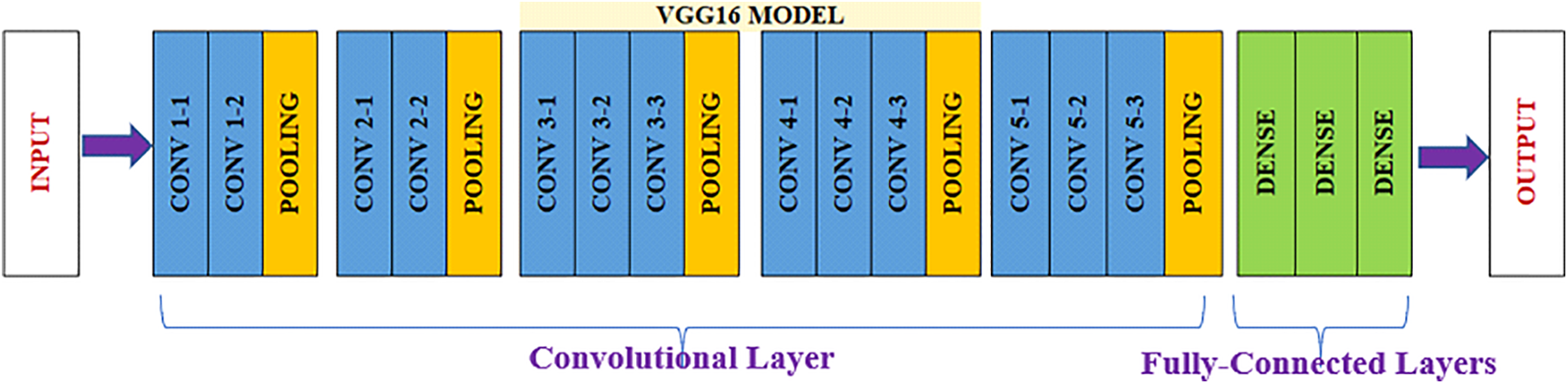
Figure 8: VGG16 base model architecture

The study utilizes the VGG16 model’s robust feature extraction and hierarchical learning to classify malware threats. Training the model on carefully selected malware datasets is anticipated to yield accurate predictions, leveraging its exceptional performance in many computer vision tasks. This initiative seeks to enhance malware detection, promote cybersecurity, and safeguard against emerging threats.

4  Methodology

The subsequent section outlines the approach employed in designing and implementing the VGG16 CNN model for our research on classifying malware attacks.

4.1 Data Preprocessing

The malware dataset has undergone a rigorous procedure to correct its form and content and prepare it for analysis. This includes solving missing values, inconsistent values, and data attributes. Predictive variables are categorized appropriately to enhance their usefulness in developing machine learning algorithms. After this cleaning process, the data set is split into a training set and a test set to validate model accuracies prominently.

In our particular approach, the malware binaries are transformed into grayscale images, and each binary file is read in binary. The byte sequences are then converted to pixel intensity, thus making sense of the malware samples and providing visual representations of them. In some cases, the images may be of different sizes, and to ensure that the essential characteristic of each sample is maintained, the images are resized to, for example, 64 × 64 or 128 × 128. This standardization makes input entry into a VGG16-based CNN possible.

4.2 Feature Extraction

Extracting features in deep CNNs for classifying Android malware based on images includes multiple essential processes. Initially, the dataset comprising photos of Android malware samples must be gathered and prepared. This could include adjusting image sizes to a uniform dimension, converting them to grayscale or RGB format, and standardizing pixel values within a specific range. Subsequently, feature extraction utilizes a pre-trained CNN model like VGG16.

Our approach is to transform the tabular malware data into convenient image formats for CNNs. This methodology consists of several key steps:

1.   Data Normalization: Let us start by normalizing the fundamental values of the tabular dataset into a standardized value. It is essential to refrain from having some of the features represented in the image give out large numbers during the conversion.

2.   Feature Mapping: Every example of malware, described by parameters (flow duration, number of packets, etc.), is located in a fixed-size square grid. In this matrix, rows are referred different attributes, while the columns are other instances of malware. It is helpful to capture the relations between the features, and they can be input into CNN to allow CNN to capture instance patterns across.

3.   Color Encoding: To increase the data’s readability, we use color mapping to convert numerical values in the grid into RGB color values. For example, feature values can be on the gradient scale, so CNN uses color as input.

4.   Image Resizing: The generated images are resized to fit the standard input dimensions for VGG16, which are usually 224 by 224 pixels. This process preserves the aspect ratio so that all dataset images will be standard.

This methodology takes advantage of the spatial structures present in the tabular forms, which conventional machine learning may fail to identify. Converting numerical features into images enables CNNs to utilize their image classification capability, improving the detection and classification of malware.

4.3 Model Architecture

The VGG16 model, with its pre-trained weights from the ImageNet dataset, is a practical choice for malware classification. In this framework, the model’s layers are primarily frozen. In contrast, the input layer is adjusted to accommodate the malware dataset volume, and the output layer is fine-tuned to reflect the number of malware classes. For a four-class classification task, categorical cross-entropy is the appropriate loss function, with optimizers like Adam or RMSprop utilized alongside a carefully selected learning rate. During training, it’s crucial to monitor the number of batches and epochs to optimize computational resources and ensure convergence of the training set. Model performance is evaluated using metrics such as loss and accuracy, which provide insights into the model’s understanding of malware attack structures. In-depth evaluation involves calculating accuracy, precision, recall, and F1 score, complemented by confusion matrices to visualize performance across different virus classifications. These assessments highlight the need for adjustments in fine-tuning methods or hyperparameters to enhance model stability and classification effectiveness.

The study aims to leverage the trained VGG16 model for generating predictions on new, unseen instances of malware, facilitating deeper analysis of its outputs to improve detection capabilities. Thorough performance estimation is essential before deploying deep convolutional neural networks (CNNs) for image-based Android malware classification. Traditional validation techniques, such as cross-validation and hold-out validation sets, are employed to mitigate overfitting risks. Cross-validation divides the dataset into multiple subsets, allowing diverse training and validation scenarios, while hold-out validation provides a final assessment of the model’s generalization ability post-training. By utilizing the VGG16 architecture, which is well-known for its success in image classification, this study incorporates best practices to enhance model performance. Techniques such as learning rate schedules are implemented to aid convergence during training, and early stopping is employed to monitor validation loss and prevent overfitting. Additionally, the study will explore architectural modifications aimed at improving stability when encountering adversarial examples and varying representations of malware.

Hyperparameter tuning remains a critical focus, as it helps identify optimal configurations for achieving the best performance and minimizing loss. The analysis will delve into the model’s behaviors and the relevance of individual features, including visualizing learned features to understand decision-making processes, thereby shedding light on specific classification outcomes.

4.4 Model Architecture Design

This study’s CNN design utilizes the VGG16 pre-trained model trained initially on ImageNet. The VGG16 model is imported with weights initialized using ‘imagenet’ weights. The model is customized for individual tasks by excluding the fully linked layers using the include_top parameter set to false. The input shape is specified as (IMG_SIZE, IMG_SIZE, 3), indicating the preferred size of input images and the quantity of color channels. This setup enables incorporating VGG16’s convolutional layers while tailoring the model to the specific goals of the study. The work gains advantages by including the basic model VGG16, which has learned rich feature representations from a broad dataset such as ImageNet. This provides a solid starting point for additional task-specific layers and potential fine-tuning. Moreover, Fig. 9 shows the model architecture.

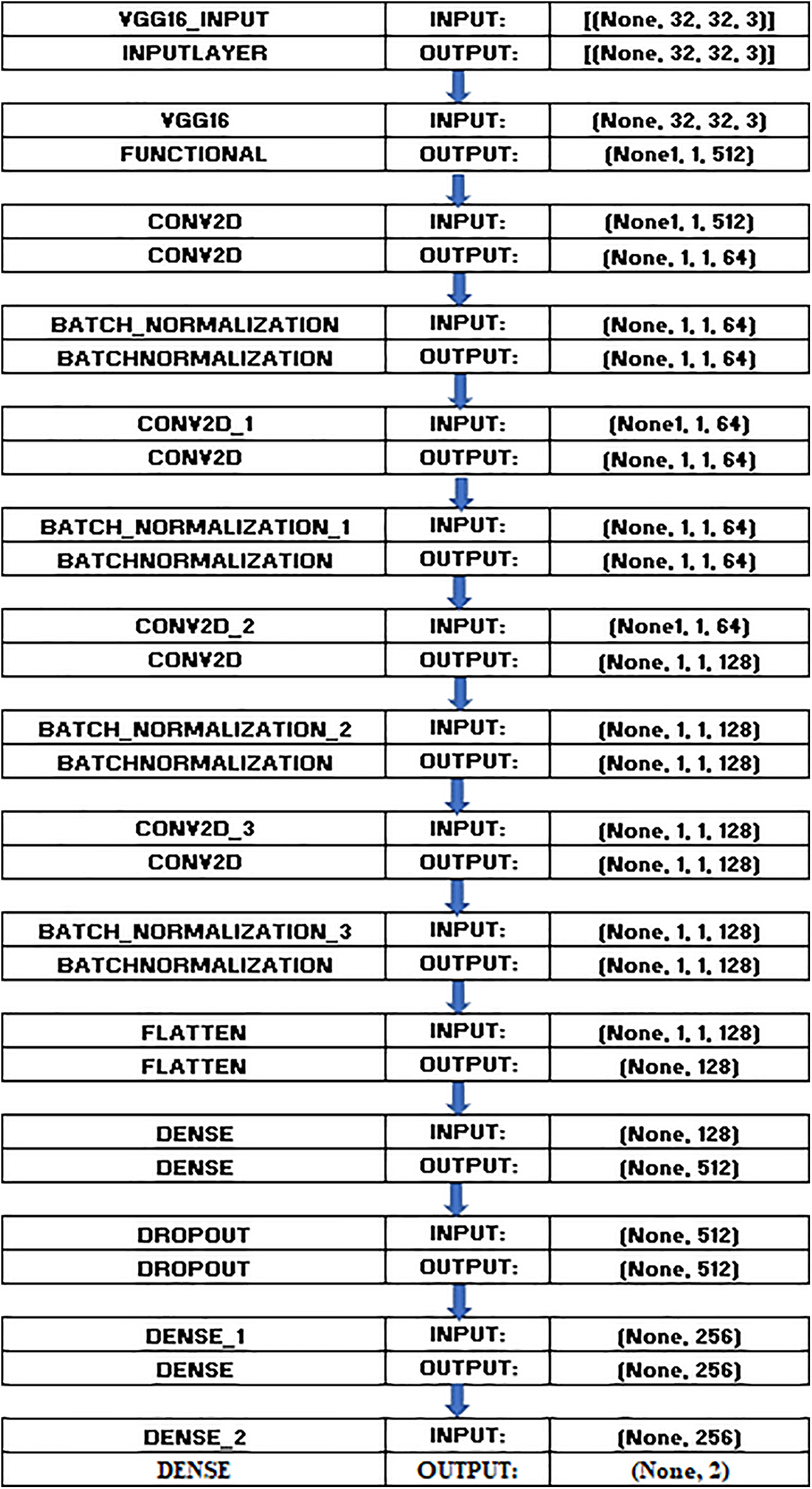
Figure 9: Proposed model architecture

The architecture of the VGG16 model has been extended with extra convolutional layers to deepen the feature learning process. All these additional layers are Conv2D configurations having predefined parameters where kernel size is 3 × 3, the activation function is ReLU, and padding is set to “same” to maintain the spatial resolution of the input. To optimize the model, batch normalization layers are added after each Conv2D layer. Such standardization of activations tends to provide the stabilization and acceleration of the training phase and, thus, improves the general work of the chosen model.

By adding the supplementary convolutional layers to the VGG16 architecture, it is apparent that the extraction of features and the accuracies have been greatly improved. Especially the architecture has added three more Conv2D layers with 64, 128, and 256 filters. Both layers use the filter size of 3 × 3, ReLU activation function, and ‘same’ padding, which maintains the spatial size of the input feature map. This makes it easier for the network to detect data details, such as the edges in images in domains like image classification, where edge details may form the basis for making accurate predictions.

The first additional layer with 64 filters is the first step of high-level feature extraction since a simple architecture with deep convolutional layers will be used to represent a pile of features. As the layers advance, the second layer, with the setting of 128 filters, enhances the possible pattern recognition of the network to detect and comprehend deeper structures combined and abstract from the features discerned by the first layer. However, the final third part, with 256 filters, examines the representation more deeply. It makes the model dig into the most subtle details to distinguish between classes in sophisticated datasets, which are typical for malware classification.

In addition, the use of Batch Normalization layers, incorporated after each convolutional layer, significantly contributes to stabilizing the training process. This is why the additional layers they introduced offer operations to normalize the output of each layer, decreasing internal covariate shifts to minimize variance during training. Besides, this brings about faster convergence and reduces the overfitting testing problem, which is a huge problem when using deep learning models. Getting trapped in the noise of training data is often a pitfall of overfitting, and thus, having these normalization layers as part of the model is essential for generalization.

The proposed model incorporates three additional convolutional layers to enhance the feature extraction capabilities. The first additional layer is a Conv2D layer with 64 filters of size 3 × 3, using the ReLU activation function and the same padding. The second additional layer is another Conv2D layer, this time with 128 filters of size 3 × 3, also utilizing the ReLU activation function and the same padding. Finally, the third additional layer is a Conv2D layer with 256 filters of size 3 × 3, again employing the ReLU activation function and the same padding.

The improvements that arise from these additional layers are especially relevant in scenarios that involve classification if precision is essential. Enhancements of feature extraction add extra capability of parsing refined distinctions rooted in the provided input, enhancing the predictive reliability of the model. This is especially useful in niche domains such as malware detection, where the capacity to categorize malicious and nonmalicious samples correctly has key consequences. On balance, these measures are introduced as additional layers, and optimizing the division of the VGG16 architecture increases the readiness of the model for the classification of complex patterns.

4.5 Compilation and Model Summary

Two notable schemas for the model architecture are highlighted. The first leverages pre-trained VGG16 features, supplemented by additional CNN layers to address task-specific features. Batch normalization layers are included to enhance regularization and training efficiency. As a deterministic binary classification model, it incorporates dense layers and an output layer for precise predictions. Key parameters are carefully selected, with a batch size of 32 over 50 epochs, a learning rate 0.001, and the Adam optimizer for accelerated convergence. Early stopping is employed to prevent overfitting by monitoring validation loss.

To enhance accuracy, k-fold cross-validation will be utilized, allowing for the identification of significant factors influencing BTC evaluation. This technique divides the data into subsets for robust testing across various datasets, improving malware detection capabilities. Additionally, model regularization methods will be explored to enhance generalization alongside data augmentation techniques to address class imbalance. The experiments are conducted in Google Colab, benefiting from dynamic computational power. Training the proposed model averages around 0.2 h over 50 iterations, facilitating efficient data flow and computations. These enhancements aim to contribute to the effective identification and categorization of malware.

4.6 Model Evaluation

To assess our model’s efficacy, we will use several commonly utilized evaluation metrics:

•   Accuracy: Accuracy is considered the primary assessment statistic, as it measures the overall correctness of forecasts.

•   Precision: Precision is a statistical measure quantifying the ratio of correctly predicted positive cases to the expected number of positive cases.

•   Recall (Sensitivity or True Positive Rate): The recall metric quantifies the proportion of correctly predicted positive events relative to the number of positive instances.

•   F1 Score: The F1 score is obtained by calculating the harmonic mean of accuracy and recall. The proposed method provides a unified metric that effectively balances accuracy and recall. The F1 score is optimal when seeking a trade-off between precision and recall.

•   Area Under the Receiver Operating Characteristic Curve (AUC-ROC): The area under the receiver operating characteristic curve (AUC-ROC) is a key performance metric for binary classification. It measures the model’s ability to distinguish between positive and negative instances across various probability thresholds. AUC-ROC values above 1 indicate better classification performance.

•   Confusion Matrix: Using a confusion matrix allows us to evaluate the efficacy of our classification model by providing a detailed analysis of predicted vs. observed class labels. This analysis includes metrics for true positives, false positives, and false negatives. The confusion matrix is set up for binary classification of benign and malicious labels.

The obtained results are shown in the following Table 3:

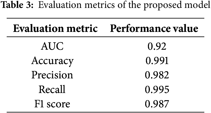
Our model demonstrates exceptional training performance, achieving an accuracy rate of 99.25%. This indicates the effective classification of most training events. The high precision reflects the model’s ability to discern patterns and distinctive features in the training dataset, leading to accurate predictions.

The curve in Fig. 10 shows our model’s training and validation accuracy. After training, we evaluated its performance on a separate testing dataset, achieving a notable testing accuracy of 98%. This high accuracy indicates the model’s effectiveness in reliably classifying unseen samples, highlighting its robustness and ability to generalize from the training data.

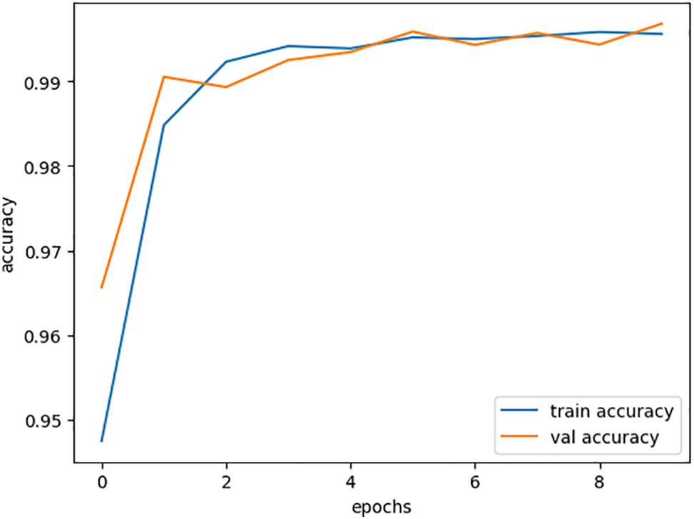
Figure 10: Training and validation accuracy performance

Fig. 11 displays the ROC curve, where a value closer to 1 signifies greater accuracy, while values near 0.5 suggest suboptimal performance. Our model achieves a value of 1, indicating exceptional classification performance.

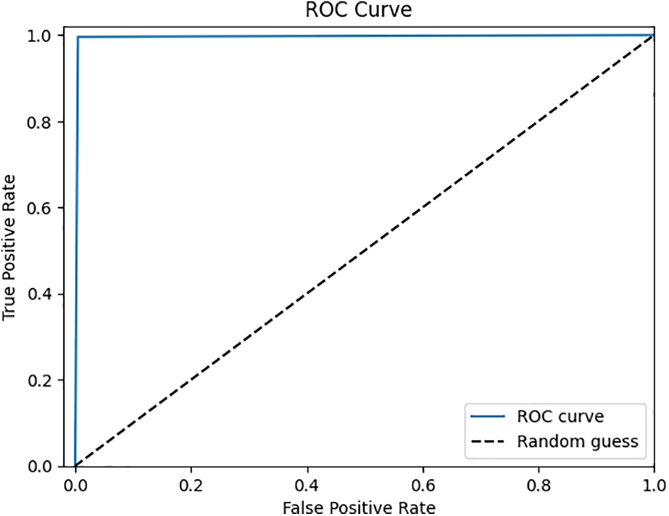
Figure 11: ROC-AUC curve

Fig. 12 shows the confusion matrix. Of 11,066 instances, 10,066 were correctly identified as benign, with only 53 misclassified. For the attack class, 13,525 instances were accurately classified, while just 54 were incorrectly labeled as benign.

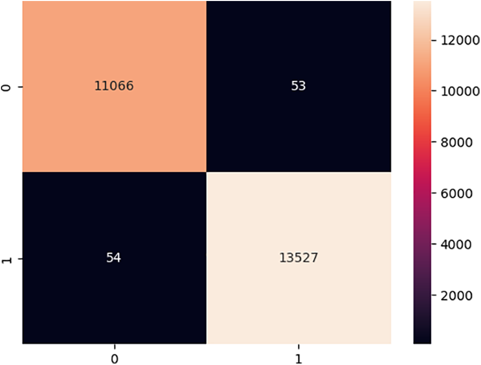
Figure 12: Confusion matrix for binary malware classification

Confusion matrix analysis shows the model’s strong capability to differentiate between malware types with high accuracy and recall rates. However, it is essential to address potential misclassification cases, as understanding these weaknesses could enhance the model’s performance for practical applications where malware threats are constantly evolving. The ROC curve and AUC results support the model’s stability, with an AUC of 1 indicating optimal sensitivity and specificity in detection. The training process demonstrates strong convergence, suggesting effective learning of malware-related patterns without overfitting.

5  Comparative Analysis

The rise of malware threats targeting Android platforms has prompted extensive research into effective identification and classification methods. As illustrated in Table 4, this comparative analysis reviews the effectiveness of various machine learning and deep learning approaches in enhancing malware detection rates. Our proposed method, Deep Convolution Neural Networks for Image-based Android Malware Classification, demonstrates superior performance on the CIC-AndMal2017 dataset. A common strategy in antivirus detection is convolutional neural networks (CNNs), which have achieved accuracy rates as high as 99% in detecting malicious patterns in Android applications. This indicates that deep learning techniques generally outperform traditional methods. For instance, the GA-StackingMD approach, which uses a stacking ensemble technique, achieved an accuracy of 98.66%. However, this method’s complexity can hinder performance compared to more straightforward CNN models.

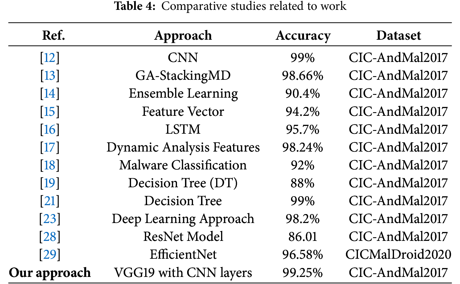
Our model, incorporating VGG19 with additional CNN layers, achieves an impressive accuracy of 99.25%. This improvement reflects enhanced feature extraction capabilities essential for identifying subtle malware variations. The depth of the VGG19 architecture facilitates superior detection of complex patterns, resulting in greater accuracy and resilience against interference. In comparison, other studies using ensemble learning techniques have achieved about 90.4% accuracy, while feature vector methods for family classification reached 94.2%, underscoring the importance of feature selection but falling short of CNN-based approaches. Innovative Long Short-Term Memory (LSTM) networks have shown promise with 95.7% accuracy, yet they are less effective than CNNs for image representation tasks. Dynamic analysis methods have also reached 98.24% accuracy through real-time behavior assessment. Still, our image-based technique allows for faster evaluations without execution, making it more suitable for large-scale applications. Control flow analysis using deep neural networks has shown 92% accuracy, while Decision Trees (DT) achieved 88%, limited by their complexity and lack of adaptability. Our approach significantly outperforms previous studies, including those using sparse binary images for IoT malware detection, and achieves 99.25% accuracy on the CIC-AndMal2017 dataset, significantly surpassing the earlier 11.1% error rate. Additionally, ResNet and EfficientNet achieved 86.01% and 96.58% accuracy on different datasets, but our VGG19-based model demonstrates superior performance in malware classification.

Our Deep Convolution Neural Networks for Image-based Android Malware Classification sets a new benchmark with an accuracy rate of 99.25% on the CIC-AndMal2017 dataset, marking a significant advancement in malware detection. We enhance efficacy through practical deep-learning implementation by combining VGG19 architecture with CNN layers. Our approach addresses common challenges in Android malware classification and lays a robust foundation for future research and development. Additionally, our methodology incorporates essential preprocessing steps, such as coordinating the conversion of malware binaries, to ensure image consistency and customization for the modified VGG16 model. These improvements and preprocessing techniques address class imbalance issues in malware datasets, leading to better identification outcomes. Our innovative method integrates the extended VGG16 framework with a proposed preprocessing scheme, representing an optimized solution for effective malware detection.

6  Limitations and Future Directions

The proposed use of deep Convolutional Neural Networks (CNNs) for Android malware detection through image-based classification marks a significant improvement over traditional signature-based method. While signature detection effectively identifies known malware, it struggles with new or modified threats, necessitating frequent updates and consuming considerable resources. In contrast, CNNs enhance adaptability by learning from new data without complete retraining and can extract features from complex, unstructured data like malware images, improving detection capabilities. However, CNN-based approaches face challenges, such as generalization issues seen in models like FalDroid and GA-StackingMD, which may not perform well across diverse real-world scenarios. Hyperparameter tuning can be time-consuming and resource-intensive, and model performance may vary in chaotic environments. Although the proposed VGG16 model with additional CNN layers incorporates features like batch normalization and dropout to enhance flexibility and stability, it still grapples with balancing efficiency and adaptability across different datasets, raising concerns about overfitting and the need for extensive, diverse training datasets.

Future research should focus on several areas to improve deep CNNs for Android malware detection. Implementing new architectures like Vision Transformers (ViTs) or advanced residual networks could enhance pattern recognition. Ensemble learning techniques like bagging, boosting, or stacking may reduce classification errors and increase reliability for challenging malware classes. Exploring adversarial training can bolster model resilience against attacks, while data augmentation techniques are essential for addressing limited training data by generating synthetic variants of known malware images. Real-world field tests are crucial for validating the practical effectiveness of these advancements, ensuring that theoretical developments translate into robust, user-centered cybersecurity tools.

7  Conclusion

This study explores the classification of Android malware using deep convolutional neural networks (CNNs) and image processing techniques, utilizing the CIC-AndMal2017 dataset, achieving impressive accuracy rates of 99.25% during training and 98% during testing. Rigorous data processing and exploratory data analysis were employed, utilizing visualizations like scatter plots and histograms to enhance understanding of the dataset. The VGG16 CNN architecture was adapted for tabular data, featuring multiple convolutional layers and fully connected layers, with a softmax activation function for multi-class classification. The model’s performance was evaluated using precision, recall, and F1 score metrics. Advantages included leveraging pre-trained VGG16 weights and implementing data augmentation techniques. At the same time, limitations highlighted the need for larger, more diverse datasets and challenges in adapting the model to new malware variants. Overall, this study demonstrates the effectiveness of deep learning in Android malware detection and contributes valuable insights for advancing classification algorithms in cybersecurity.

Acknowledgement: Authors would like to thank the Deanship of Scientific Research at Princess Nourah bint Abdulrahman University, through the Research Funding Program, Grant No. (FRP-1443-15) for funding this research.

Funding Statement: This research was funded by the Deanship of Scientific Research at Princess Nourah bint Abdulrahman University, through the Research Funding Program, Grant No. (FRP-1443-15).

Author Contributions: Study conception and design: Amel Ksibi, Mohammed Zakariah, Latifah Almuqren, Ala Saleh Alluhaidan; data collection: Mohammed Zakariah, Latifah Almuqren; analysis and interpretation of results: Amel Ksibi, Ala Saleh Alluhaidan; draft manuscript preparation: Mohammed Zakariah, Ala Saleh Alluhaidan. All authors reviewed the results and approved the final version of the manuscript.

Availability of Data and Materials: Data is freely available and can give access on request.

Ethics Approval: Not applicable.

Conflicts of Interest: The authors declare no conflicts of interest to report regarding the present study.

References

1. Sun N, Ding M, Jiang J, Xu W, Mo X, Tai Y, et al. Cyber threat intelligence mining for proactive cybersecurity defense: a survey and new perspectives. IEEE Commun Surv Tutorials. 2023;25(3):1748–74. doi:10.1109/COMST.2023.3273282. [Google Scholar] [CrossRef]

2. Saidia Fascí L, Fisichella M, Lax G, Qian C. Disarming visualization-based approaches in malware detection systems. Comput Secur. 2023;126(17):103062. doi:10.1016/j.cose.2022.103062. [Google Scholar] [CrossRef]

3. Ravi V, Alazab M. Attention-based convolutional neural network deep learning approach for robust malware classification. Comput Intell. 2023;39(1):145–68. doi:10.1111/coin.12551. [Google Scholar] [CrossRef]

4. Alsuwat E, Solaiman S, Alsuwat H. Concept drift analysis and malware attack detection system using secure adaptive windowing. Comput Mater Contin. 2023;75(2):3743–59. doi:10.32604/cmc.2023.035126. [Google Scholar] [CrossRef]

5. Ayele YZ, Chockalingam S, Lau N. Threat actors and methods of attack to social robots in public spaces. In: HCI for cybersecurity, privacy and trust. Cham: Springer Nature Switzerland; 2023. p. 262–73. doi:10.1007/978-3-031-35822-7_18. [Google Scholar] [CrossRef]

6. Mehmood M, Amin R, Ali Muslam MM, Xie J, Aldabbas H. Privilege escalation attack detection and mitigation in cloud using machine learning. IEEE Access. 2023;11(10):46561–76. doi:10.1109/ACCESS.2023.3273895. [Google Scholar] [CrossRef]

7. Duraibi S. Enhanced image-based malware classification using snake optimization algorithm with deep convolutional neural network. IEEE Access. 2024;12(9):95047–57. doi:10.1109/ACCESS.2024.3425593. [Google Scholar] [CrossRef]

8. Mercaldo F, Martinelli F, Santone A. Deep convolutional generative adversarial networks in image-based Android malware detection. Computers. 2024;13(6):154. doi:10.3390/computers13060154. [Google Scholar] [CrossRef]

9. Liu Y, Fan H, Zhao J, Zhang J, Yin X. Efficient and generalized image-based CNN algorithm for multi-class malware detection. IEEE Access. 2024;12(5):104317–32. doi:10.1109/ACCESS.2024.3435362. [Google Scholar] [CrossRef]

10. Ashawa M, Owoh N, Hosseinzadeh S, Osamor J. Enhanced image-based malware classification using transformer-based convolutional neural networks (CNNs). Electronics. 2024;13(20):4081–1. doi:10.3390/electronics13204081. [Google Scholar] [CrossRef]

11. Kumar S, Kumar A. Image-based malware detection based on convolution neural network with autoencoder in Industrial Internet of Things using Software Defined Networking Honeypot. Eng Appl Artif Intell. 2024;133(5):108374. doi:10.1016/j.engappai.2024.108374. [Google Scholar] [CrossRef]

12. Djenna A, Bouridane A, Rubab S, Marou IM. Artificial intelligence-based malware detection, analysis, and mitigation. Symmetry. 2023;15(3):677. doi:10.3390/sym15030677. [Google Scholar] [CrossRef]

13. Xie N, Qin Z, Di X. GA-StackingMD: android malware detection method based on genetic algorithm optimized stacking. Appl Sci. 2023;13(4):2629. doi:10.3390/app13042629. [Google Scholar] [CrossRef]

14. Arslan RS. Identify type of Android malware with machine learning based ensemble model. In: 2021 5th International Symposium on Multidisciplinary Studies and Innovative Technologies (ISMSIT); 2021 Oct 21–23; Ankara, Turkey: IEEE; 2021. doi:10.1109/ismsit52890.2021.9604661 [Google Scholar] [CrossRef]

15. Fan M, Liu J, Luo X, Chen K, Tian Z, Zheng Q, et al. Android malware familial classification and representative sample selection via frequent subgraph analysis. IEEE Trans Inform Forensic Secur. 2018;13(8):1890–905. doi:10.1109/TIFS.2018.2806891. [Google Scholar] [CrossRef]

16. Lashkari AH, Kadir AFA, Taheri L, Ghorbani AA. Toward developing a systematic approach to generate benchmark Android malware datasets and classification. In: 2018 International Carnahan Conference on Security Technology (ICCST); 2018 Oct 22–25; Montreal, QC, Canada: IEEE; 2018. p. 1–7. doi:10.1109/CCST.2018.8585560 [Google Scholar] [CrossRef]

17. Tsfaty C, Fire M. Malicious source code detection using transformer. arXiv:2209.07957. 2022. [Google Scholar]

18. Qiang W, Yang L, Jin H. Efficient and robust malware detection based on control flow traces using deep neural networks. Comput Secur. 2022;122(5):102871. doi:10.1016/j.cose.2022.102871. [Google Scholar] [CrossRef]

19. Lindorfer M, Neugschwandtner M, Platzer C. MARVIN: efficient and comprehensive mobile app classification through static and dynamic analysis. In: 2015 IEEE 39th Annual Computer Software and Applications Conference; 2015 Jul 1–5; Taichung, Taiwan: IEEE; 2015. p. 422–33. doi:10.1109/COMPSAC.2015.103 [Google Scholar] [CrossRef]

20. Pavithra J, Selvakumara Samy S. A comparative study on detection of malware and benign on the Internet using machine learning classifiers. Math Probl Eng. 2022;2022(4):4893390. doi:10.1155/2022/4893390. [Google Scholar] [CrossRef]

21. Yadav CS, Singh J, Yadav A, Pattanayak HS, Kumar R, Khan AA, et al. Malware analysis in IoT & Android systems with defensive mechanism. Electronics. 2022;11(15):2354. doi:10.3390/electronics11152354. [Google Scholar] [CrossRef]

22. Aboshady D, Ghannam N, Elsayed E, Diab L. The malware detection approach in the design of mobile applications. Symmetry. 2022;14(5):839. doi:10.3390/sym14050839. [Google Scholar] [CrossRef]

23. Zhang S, Gao M, Wang L, Xu S, Shao W, Kuang R. A malware-detection method using deep learning to fully extract API sequence features. Electronics. 2025;14(1):167. [Google Scholar]

24. Calik Bayazit E, Koray Sahingoz O, Dogan B. Deep learning based malware detection for Android systems: a comparative analysis. Teh Vjesn. 2023;30(3):787–96. doi:10.17559/tv-20220907113227. [Google Scholar] [CrossRef]

25. Kumar S, Janet B, Neelakantan S. IMCNN: intelligent malware classification using deep convolution neural networks as transfer learning and ensemble learning in honeypot enabled organizational network. Comput Commun. 2024;216(1):16–33. doi:10.1016/j.comcom.2023.12.036. [Google Scholar] [CrossRef]

26. Shelar MD, Rao SS. Enhanced capsule network‐based executable files malware detection and classification—deep learning approach. Concurr Comput: Pract Exper. 2024;36(4):e7928. doi:10.1002/cpe.7928. [Google Scholar] [CrossRef]

27. Alam I, Samiullah M, Kabir U, Woo S, Leung CK, Nguyen HH. SREMIC: spatial relation extraction-based malware image classification. In: 2024 18th International Conference on Ubiquitous Information Management and Communication (IMCOM); 2024 Jan 3–5; Kuala Lumpur, Malaysia: IEEE; 2024. p. 1–8. doi:10.1109/IMCOM60618.2024.10418339 [Google Scholar] [CrossRef]

28. Brown A, Gupta M, Abdelsalam M. Automated machine learning for deep learning based malware detection. Comput Secur. 2024;137(1):103582. doi:10.1016/j.cose.2023.103582. [Google Scholar] [CrossRef]

29. Poornima S, Mahalakshmi R. Automated malware detection using machine learning and deep learning approaches for android applications. Meas: Sens. 2024 Apr;32(1):100955. doi:10.1016/j.measen.2023.100955. [Google Scholar] [CrossRef]