
 Submit a Paper
 Propose a Special lssue
 Open Access
ARTICLE

Modified Neural Network Used for Host Utilization Predication in Cloud Computing Environment
1 Centre for Intelligent Cloud Computing, Multimedia University, Melaka, 75450, Malaysia
2 Faculty of Information Science and Technology, Multimedia University, Melaka, 75450, Malaysia
* Corresponding Author: Siti Fatimah Abdul Razak. Email:
Computers, Materials & Continua 2025, 82(3), 5185-5204. https://doi.org/10.32604/cmc.2025.059355
Received 05 October 2024; Accepted 13 December 2024; Issue published 06 March 2025
 View Full Text
 Download PDF
Abstract
Networking, storage, and hardware are just a few of the virtual computing resources that the infrastructure service model offers, depending on what the client needs. One essential aspect of cloud computing that improves resource allocation techniques is host load prediction. This difficulty means that hardware resource allocation in cloud computing still results in hosting initialization issues, which add several minutes to response times. To solve this issue and accurately predict cloud capacity, cloud data centers use prediction algorithms. This permits dynamic cloud scalability while maintaining superior service quality. For host prediction, we therefore present a hybrid convolutional neural network long with short-term memory model in this work. First, the suggested hybrid model is input is subjected to the vector auto regression technique. The data in many variables that, prior to analysis, has been filtered to eliminate linear interdependencies. After that, the persisting data are processed and sent into the convolutional neural network layer, which gathers intricate details about the utilization of each virtual machine and central processing unit. The next step involves the use of extended short-term memory, which is suitable for representing the temporal information of irregular trends in time series components. The key to the entire process is that we used the most appropriate activation function for this type of model a scaled polynomial constant unit. Cloud systems require accurate prediction due to the increasing degrees of unpredictability in data centers. Because of this, two actual load traces were used in this study’s assessment of the performance. An example of the load trace is in the typical dispersed system. In comparison to CNN, VAR-GRU, VAR-MLP, ARIMA-LSTM, and other models, the experiment results demonstrate that our suggested approach offers state-of-the-art performance with higher accuracy in both datasets.Keywords
The three main services that cloud computing provides are infrastructure as a service (IaaS), platform as a service (PaaS), and software as a service (SaaS). These services are provided to users via the Internet in accordance with the pay-and-gain policy. One of the main purposes of cloud computing is to provide the user with access to a large amount of virtualized resources [1,2]. Compute as a service, which enables customers to access different resources like hardware, software, CPUs, and apps via the internet, is one of the main characteristics of cloud computing. Cloud technology is widely employed in many aspects of life because of its biggest resource on-demand delivery, low resource cost, and flexible resource scalability [3]. Different numbers of applications have been developed using the cloud platform to improve these programs; other methods, including prediction, are employed for resource allocation. However, there are still several problems with this technology, such as resource and application balance, which could enhance system performance [4].
Predicting workload and resources is a crucial aspect of cloud management platforms and systems. Prediction processes increase accuracy rates and have a direct impact on security, service quality, economy, and management processes, all of which enhance cloud-computing performance. Load and application prediction usually describes the future behavior of resources and applications on a specific feature of the obtained knowledge base [5,6]. Performance parameters for load prediction can include metrics like CPU use, reaction time, throughput, memory utilization, and network utilization. Future prediction techniques will be separated into load prediction and application prediction. Several machine-learning algorithms that leverage cloud application background recordings for a specific amount of time are applied proactively.
Developing an intelligent resource management system based on historical data is one of the key goals of the machine learning technique [7]. One of the essential aspects for efficient resource management in cloud computing is application prediction, which accounts for future demand projections. Application prediction work is done in various domains, such as workload prediction, service-level agreement (SLA) measures, and quality of service (QoS) [8]. To quickly estimate future resource, requirements prediction techniques are crucial in cloud computing because they are precise. It is possible to predict resource management in a cloud environment with accuracy during the application process. Because of this, precise forecasting is essential for cost reduction and resource management at its best [9,10]. Most cloud providers offer scalable services that give computer resources (such as CPU, memory, and storage) on demand because Infrastructure as a Service (IaaS) provides speedy and flexible IT resources.
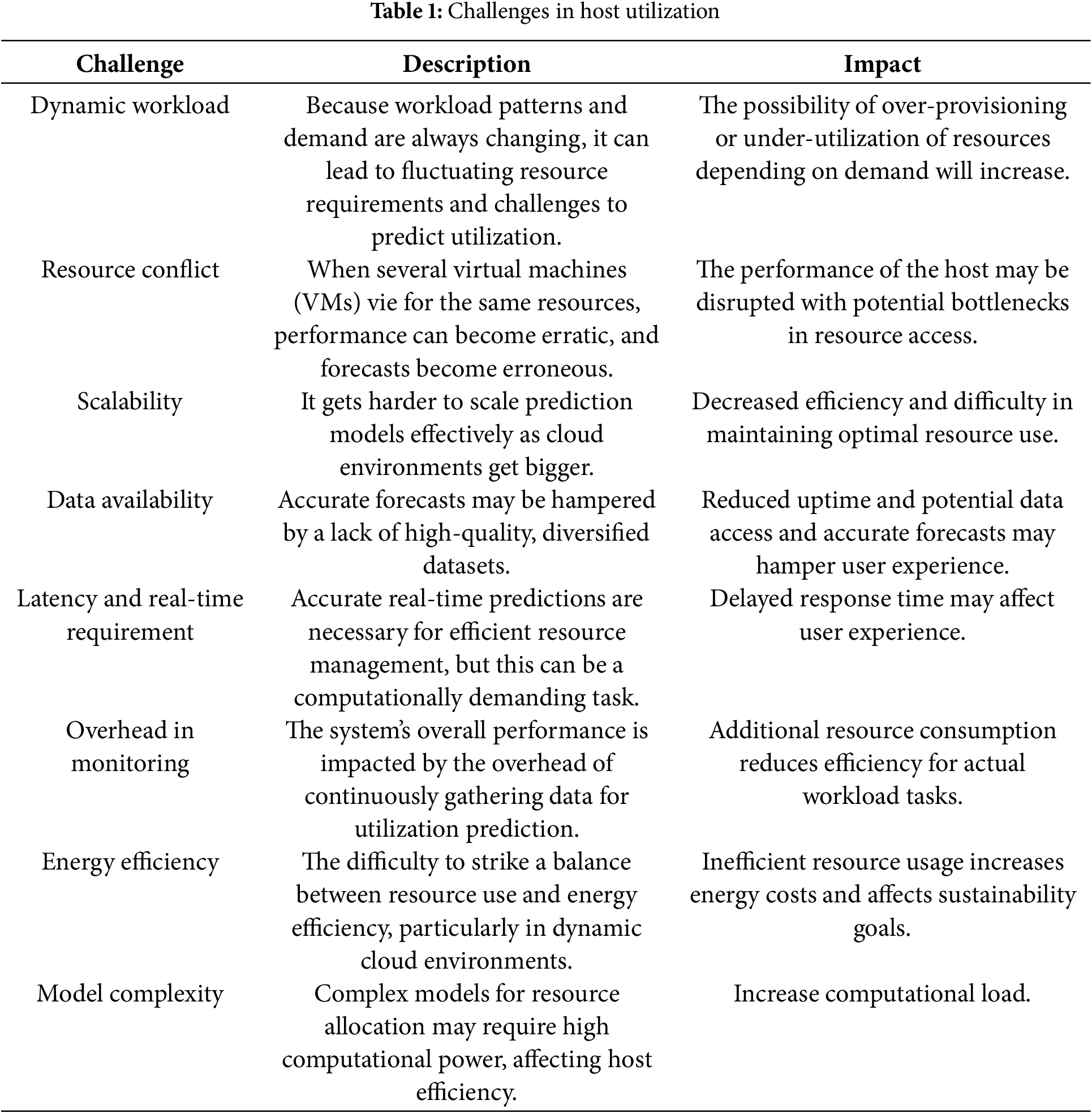
Nonetheless, the main cause of the several-minute lag is the scaling time needed to set up a virtual machine and CPU. Minimizing scaling time delays requires exact resource allocation to be predetermined. For this reason, predicting CPU and virtual machine consumption is crucial to resolve this problem [11]. Previous studies have identified challenges in host utilization, i.e., dynamic workload, resource conflict, scalability, data availability, latency etc. These challenges collectively highlight the limitations of traditional and single-architecture models, necessitating a hybrid CNN-LSTM approach that can leverage both local feature extraction and long-term memory retention to provide accurate and timely host load predictions in cloud environments. We summarize the challenges in Table 1.
Moreover, since cloud computing provides scalable, on-demand resources to accommodate changing workload requirements, it has become essential to current IT infrastructures. Effective resource management is still a major obstacle, though, since under-provisioning causes performance bottlenecks while over-provisioning wastes resources. To ensure the best possible allocation of computer resources, lower operating costs, and improve system performance, an accurate host utilization forecast is essential. A customized neural network can improve resource management, forecast host use more accurately, and support more effective, economical cloud operations. This justifies our motivation to conduct this study which aims to improve the load prediction approach to maximize the utilization of cloud resources. The contributions of this study are outlined as follows:
a) This study proposes a hybrid CNN and LSTM model for multivariate resource prediction in cloud data centers.
b) The proposed model is implemented with the activation function of scaled polynomial continuous unit, which is the main contribution of the proposed model.
c) The suggested approach is utilized in cloud data centers to anticipate host load more accurately.
d) This study calculates and contrasts the suggested hybrid model with various industry standards.
e) This study also consists of comprehensive experimental assessment for various data sets including conventional distributed system data sets and publicly accessible Google cluster trace centers within a cloud-computing environment.
The remainder of the document is structured as follows: Section 2 provides the background information required for resource prediction; Section 3 presents the proposed model; Section 4 describes the dataset and experimental results; Section 5 highlights the contribution of the proposed model, and Section 6 presents the conclusion.
Cloud computing offers flexible resource distribution according to cloud customers’ requirements. Since the demand for cloud users fluctuates over time, creating a resource-forecasting model is difficult [12]. Since cloud computing relies heavily on the round-trip time (RTT) of cloud servers, Damaševičius et al. [13] proposed a neuron fuzzy network with eight probability distribution functions to forecast RTT. This method was used to quantify the time it takes for data to travel from a source node to a destination node and back. The recommended approach boosts productivity and reduces error rates. The offloading method and prediction rate were enhanced by the author’s efforts.
To get a greater prediction accuracy rate, Kholidy et al. [14] presented the swarm intelligence-based prediction method known as SIBPA to predict resource allocations for CPU, memory, and storage consumption. The results of the suggested algorithm are contrasted with those of established algorithms including Linear regression, Neural Network and Support Vector Machines. In [15], the multi-agent system (MAS) for the cloud computing computational resource allocation system’s dynamic monitor prediction system is presented by the authors. The reasoning agent technique that is being discussed works in concert with the architectural system through its three-layer components. Many linear regressions models with lower means for the error system were shown. Based on the findings, the author claims that the Google platform achieves a respectable rate of prediction and accuracy. Because load balancing techniques and balance optimization systems are so important to cloud computing’s use of hardware resources, a concept called an LSTM (long short-term memory) encoder-decoder was proposed by Zhu et al. [16]. The authors proposed two models where the first model employs the feature context of the past workload while the second model integrates the attention mechanism into the decoder network and performs the prediction. The study uses the workload traces datasets from Alibaba and Dinda. Based on the results, it is claimed that the suggested solution works more accurately and requires a smaller sequence monitor system.
Most current estimating approaches employ a single model technique to evaluate resource consumption in the cloud data center, either underloaded or overloaded. Biswas et al. [17] proposed a New Linear Regression Model to predict future CPU utilization based on Virtual Machine (VM) consolidation process. This model demonstrates the ability to reduce energy consumption in cloud data centers by improving the utilization of resources. In cloud data centers, the load balancing technique is essential for optimizing resource use and reducing resource waste [18]. Huang et al. [19] proposed a hybrid approach to reduce energy consumption and predict load prediction via dynamic resource allocation in the cloud. The approach achieved around 98% accuracy in predicting energy consumption when validated using the SPECpower benchmark, which is an industry-standard benchmark to compare performance of servers in data centers. In another study, de Lima et al. [20] proposed an artificial neural network approach known as the TLP-Allocator. TLP refers to thread-level parallelism which improves computational efficiency and performance. The proposed method managed performed better than other state-of-the-art resource allocations methods on cloud environments in terms of overall optimal energy-delay product (EDP). To anticipate future multi-attribute host resource utilization, Abdullah et al. [21] used support vector regression (SVRT), a supervised learning technique suitable for non-linear cloud resource load forecasting. The recommended technique employed the sequential minimal optimization algorithm (SMOA) to optimize the training and regression sections using different types of datasets. The results show that the recommended approach reduces error percentage by 4%–16% and outperforms state-of-the-art approaches by between 8% and 20%, generally.
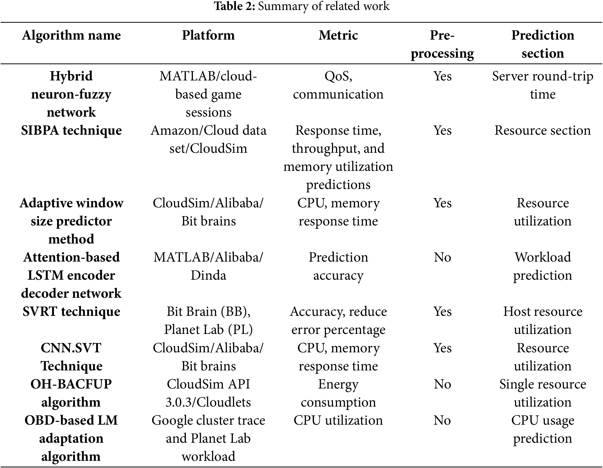
It is imperative to keep in mind that accurate data forecast the cloud data center’s resource utilization requires careful planning, which includes load balancing, workload placement, energy conservation, and scheduling. However, accurately calculating resource consumption is a considerable challenge due to the diverse range of infrastructures and dynamic nature. Consequently, Baig et al. [22] proposed a model based on methods for deep learning adaptive window size selection. Resource consumption is assessed using the sliding window size technique by estimating each trend period and contrasting it with the most recent resource use trend. The proposed estimating strategy increases prediction accuracy by 16%–54% when compared to baseline methods. Similar to Jyoti et al. [18], the authors also highlighted that the load balancing technique is one of the essential elements of cloud computing, extending the duration of the system. As a result, the Osmotic Hybrid artificial Bee and Ant Colony (OH_BAC) algorithm was introduced in [23]. The proposed method is a cross between an artificial beehive and an ant colony, as it decreases the quantity of virtual computers in use and ultimately increases the lifetime of the network. To forecast resources, the author employs simple linear regression and optimal piecewise linear regression. Then, based on the forecast results, it selects the most appropriate virtual machine (VM) for maximum utilization. The recommended algorithm improves network stability and system minimization over the classical algorithm. According to Bilski et al. [24], previous research attempted to predict cloud computing load prediction using the Levenberg-Marquardt (LM) and Gradient Descent (GD) algorithms. However, the model suffers from high computational complexity, like classic LM model. Hence, the authors proposed a vector calculations approach to significantly reduce the LM computational time when tested on different feedforward networks topologies. The model yields shorter training time compared to the classic LM. Javadpour et al. [25] proposed a method called Dynamic Voltage and Frequency Scaling (DVFS) which migrates tasks under certain situations to improve network performance. Experimental results demonstrate that the method reduces power consumption but with a longer working period which generates better profit for cloud providers. Table 2 displays a summary of related work.
We know that the LSTM model, which is used for temporal information, maps important time into separable space in order to provide predictions, and that CNN is a useful technique for removing noise and accounting for correlations between variables and multivariate data. Our proposed model uses CNN-LSTM to predict virtual machine (VM) and CPU use. A multivariate time series that is recorded over time, VM usage contains irregular patterns of both spatial and temporal information across variables [26,27]. The recommended models that are used for resource prediction metrics are CPU and RM. The proposed model architecture is presented in Fig. 1.
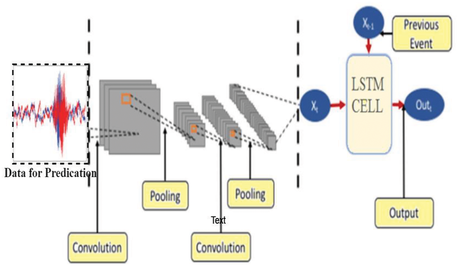
Figure 1: Proposed model architecture
In the initial step of input data analysis, the linear interdependencies between the multivariate variables are filtered using the VAR regression approach. Next, the leftover data are computed and incorporated into the CNN layer. It acquires the complex properties of every CPU and virtual machine component, uses LSTM to extract the temporal data of irregular time series components, and generates a prediction. Since the multivariate time serious data are split into linear and nonlinear parts, we can ascertain the following.
In the spatial part model, CNN was used to extract features. A hybrid CNN-LSTM model was then applied for the input process, which is appropriate for modeling temporal information after the final prediction has been entirely formed. We initially address the commonalities between these two models, then go on to multivariate workload prediction in cloud data centers by introducing our own approach. Vector autoregressive models are intended for forecasting or prediction purposes because of the way their steps are constructed, which requires values from the preceding variable in order to proceed when the present values of a set of variables are partially explained. The main purpose of this model is to elucidate the joint producing mechanism of the variable [28,29]. The arrangement of every variable in the current or previous logs’ liner function.
In Eqs. (3)–(6), the RM movement in CPU usage is t − 1 (the lag number in this section is 1), and the CPU is represented by the values y1(t), y2(t), y3(t), and y4(t); likewise, the CPU is represented by the values y1(t−1), y2(t−1), y3(t−1), and y4(t−1). The constant terms are a1, a2, a3, and a4, etc. whereas e1, e2, e3, and e4 are the four error words that are employed. They have h coefficients.
We establish the order p for the two series prior to the VAR model’s estimate section. The vector auto regression (VAR) model is a comprehensive, versatile, and very significant method for examining multivariate time series [30–33]. This particular kind involves delaying the test. Making use of the univariate multivariate time series using the autoregressive approach. The VAR model is one of the most flexible for forecasts since it established the criteria future path of a particular variable in the system. Impulse response study of VAR lag order is a crucial preliminary step in calculating impulse response using vector autoregressive models [34–36]. In this work, we have opted to estimate parameters using the AIC measure as in Eq. (7).
When it comes to the degree of freedom, the likelihood function’s value is displayed by the LN (L < X) notation, which represents the parameters used in the equation. When we have a compact model and have an AIC value, we obtain better outcomes and a better model. The residual values are calculated and then determined to the ensuing CNN-LSTM model. The nonlinear elements are anticipated to persist since the VAR model detected the linear trend [34,35]. The convolutional neural network (CNN), which is modeled after the human brain system, performs optimally in a wide range of applications. CNN’s two main characteristics are sparse connections and shared weight typical. The convolutional layer, the subsampling or pooling layer, and the fully connected layer which is utilized for classification—are the three computational layers in which CNN is used as a hierarchical model [32]. This type of neural network is specialized and designed to operate with data that has multiple dimensions, such as two or three. A 1D CNN can read input out of order and automatically identify the relevant pieces in the time series-forecasting problem. A convolutional hidden layer CNN model operating on a 1D sequence is referred to as a CNN in one dimension. When given sequence numbers as input, a 1D CNN may read it and finally determine the important characteristics for time series or forecasting applications. 1D CNN is quite good at creating topographies from a fixed-length portion of the whole dataset; regardless of the location of the data segment, it will work correctly in the relevant area for any application [36,37].
Eq. (8), which is the result of vector y1, represents the lengthy input sequence in some cases. The second convolutional layer is placed after the first.
Eq. (9) shows the highest possible layer of pooling. R is the pooling size that is less than the input y, and T is the stride that determines how far to move the area of input data.
The LSTM layer, which deduces the properties gathered by the convolutional part of the proposed model, comes after the pooling and convolutional layers. A flatten layer is positioned between the convolutions layer and the LSTM layer. Its purpose is to compress successive mappings into a single one-dimensional vector [38]. CNN is known to be composed of several layers, the lowest of which is CNN-LSTM. CNN-LSTM stores qualities of power that must be restored with the assistance of CNN and LSTM combine memory units that preserve previous buried states in order to create a theory that is resistant to microorganisms. long-term memory. This feature facilitates the easy determination of the temporal relationship on a long-term sequence by transferring the output values from the preceding CNN layer to the gate units. The LSTM network can predict power consumption by tackling the issues of vanishing gradient and explosion. Four interacting neural networks make up the LSTM cell: one for the input, forget, input candidate, and output gates. A vector with element values ranging from zero to one is produced by the forget gate. Because it can handle evaporation and explosion inclination issues, an LSTM network is appropriate for power demand prediction [39,40].
The LSTM cell contrast is made up of four neural interactions networks, every one of which is a gate. The function depicted in Fig. 2 and denoted by the same symbol is the logistic function, which is also referred to as the scaled polynomial constant unit activation function. The model’s ability to be nonlinear is due to the activation function. We’ve already discussed the two property values of the LSTM: concealed condition. The cell’s fluctuating H(t) value and C(t) presentation of the cell state enable long-term memory maintenance. Information can be added to or removed from the cell state by LSTM. To display the cell state C(t), for instance, it can connect input X(t) for the prior concealed state H(t−1). The cell can remember or disregard the use of X(t) and H(t−1) thanks to this function. Ascertain the input value feed for input sections I(t) and I(t) to the cell state C(t). When it serves a forgetter that is multiplied to the call state, it employs a separate time step to eliminate values that are not needed for prediction and keep those that are. The output gate o(t) also selects the exit based on the process of the cell state, as can be seen in the below. The instruction above explains the LSTM gate and its operation conditions. The activation function that provides the model with its nonlinear capabilities is the fir logistic function, which is also represented in Fig. 3 using the same notation. It is also referred to as the scaled polynomial constant unit. Consequently, we used the altered activation function in this model. In the next step, the input gate and candidate gate work together to create the new state cell, or State [41]. As stated in the comping section, the next step in this part is to use the scaled polynomial constant unit in the input gate and the hyperbolic tangent in the input candidate as the activation function for the renewed cell state. The four stages of the proposed hybrid CNN-LSTM model prediction approach include data preparation, model rectification, model fitting, and model estimate and prediction. As was already indicated, the algorithm passes the residual value calculated by the CNN-LSTM model. The recommended approach divides each sample into a four-time phase and the CNN model is used to infer each subsequence from a pair of subsequences so that the LSTM can put together the interpretation from the subsequences. The CNN was set up to assume two parts per subsequence, with four possible outcomes, after this subsequence was separated into two pieces. Next, a time-distributed wrapper layer was placed over the whole CNN model to ensure that it applied to each subsequence of the sample. The LSTM layer, which used fifty blocks or neurons, then assessed the result, and finally the dense layer generated the prediction. Below, Fig. 2 illustrates the operation of the active function [42,43].
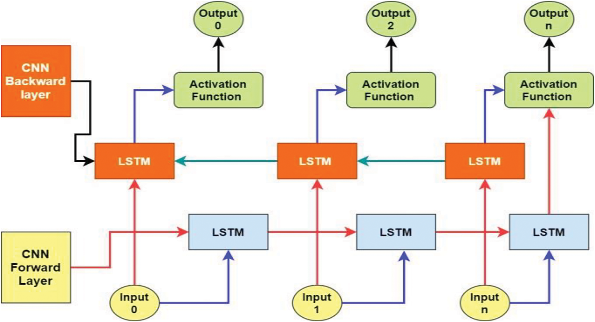
Figure 2: Activation function
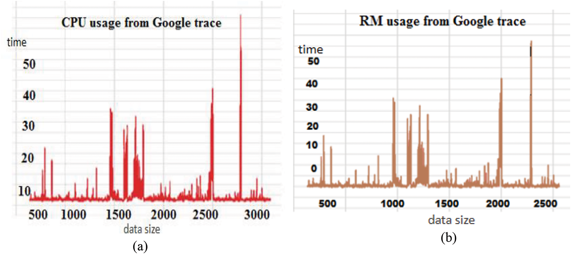
Figure 3: CPU mean load forecast: (a) CPU usage and (b) RM usage
The LSTM block and CCN layer adopt the rectified linear unit and scaled polynomial constant unit activation function [43–45]. The scaled polynomial constant unit activation function was defined by Kiseľák et al. [46] in 2021 and goes by that name. The network is trained with a batch size of 1 for 100 epochs. The ReLU activation function can significantly lessen the fading gradient issue when X delivers the input to the neuron.
The proposed modified algorithm overall complexity can be expressed as follows:
It should be emphasized that as the number of layers and neurons increases, the computational complexity increases significantly. Additionally, the algorithm depends on T iterations. Therefore, as the value of T increases, so does the complexity.
4 Experimental Results and Analysis
This section presents various results, comparing the prediction performance of our suggested model with four models, i.e., ARIMA-LSTM, VAR-GRU, VAR-MLP, and CNN, and presents the prediction effectiveness of each model. The primary justification for comparing these methods is that, according to earlier research, they yield effective results.
The workload provides time stamps for the execution and completion of various actions as well as data arrival. We examine and forecast the CPU and RM resource utilization parameters in this study. We produce and examine the out-of-sample forecasts for the upcoming 80 (fifty minutes), 200 (sixty minutes), and 400 (one hundred and twenty minutes) steps. Values for resource utilization are combined every 4 s. Based on a cluster of over 12,500 machines, Google Cluster Traces give information on the arrival times of various jobs at the center over a 29-day period. For the purpose of training the resource prediction models, we collected 70,800 samples over the course of seven days. The following thirty (4-min) time series samples are available as validation data to help with parameter selection. Prior to that, in order to train the network, we first preprocessed the data using a method called standardization, which involves dividing the training data’s standard deviation and removing its mean value [47]. When gradient descent is employed to the networks, ascending methods can benefit in combination and significantly enhance model performance. To ensure a fair comparison, standardization was performed to all linked methodologies during the experiment.
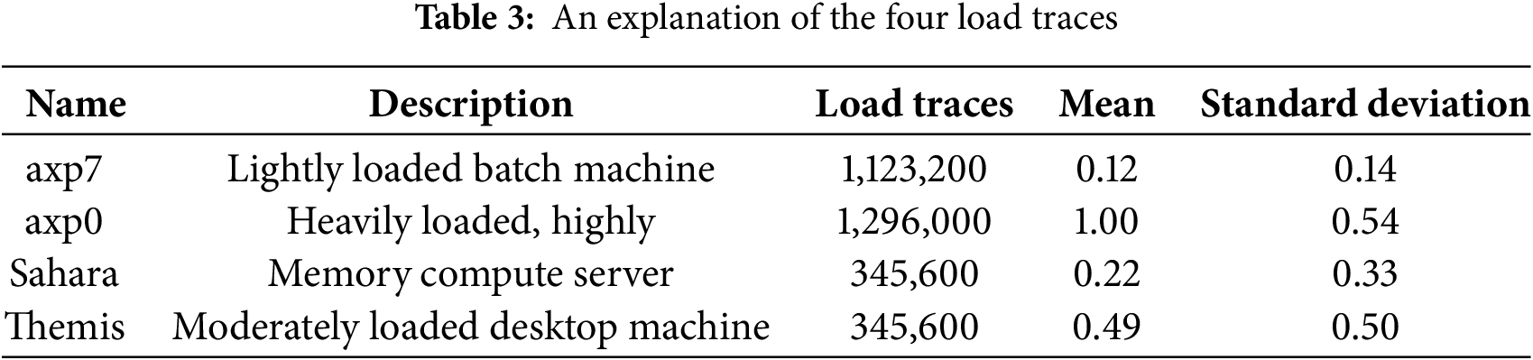
Table 3 lists the parameters selected by the validating set for 670,000 tasks. Approximately 4 million task occurrences were tracked by the data set for a period of 12,500 machines darning 29 days. These parameters ensured that the load traces selected for evaluation represented a variety of realistic scenarios, providing a comprehensive assessment of the hybrid model’s accuracy, adaptability, and robustness under diverse workload conditions. Google trace gathered more than 10 metrics, including CPU use, allocated memory, page-cache memory usage, and disk I/O. disk space and time. We are only able to anticipate the CPU and RM use values, much like the previous approaches.
An exponentially segmented pattern, a metric used to quantify the host load fluctuation across successive time intervals whose durations rise exponentially, was employed to make the result comparable with other models [48]. The mean segment squared error (MSSE), which is defined as follows, was used to measure how well mean load prediction performed. The predicted means value is the true value and is represented by the baseline segment in Eq. (16).
The sum of the segments’ values within the prediction interval where si = b, 2i−2, s =
After first projecting the load over a single load interval in the simulation, we converted the prediction into a load pattern. The findings of the suggested model are contrasted in Fig. 3a with the cutting-edge method, which forecasts the mean load throughout the subsequent future time intervals shown in Fig. 3b. There is just one load interval displayed for the procedure. A thorough comparison of our suggested model with other models, along with mean load projections for a given future interval, is shown in Fig. 3b. Based on those data, our model generates better outcomes than any of the five single periods due to its nonlinear generalization capacity. Due to the significant host load fluctuation and noise, the MSSE’s length is not smooth; Fig. 4 displays the findings of that particular section.
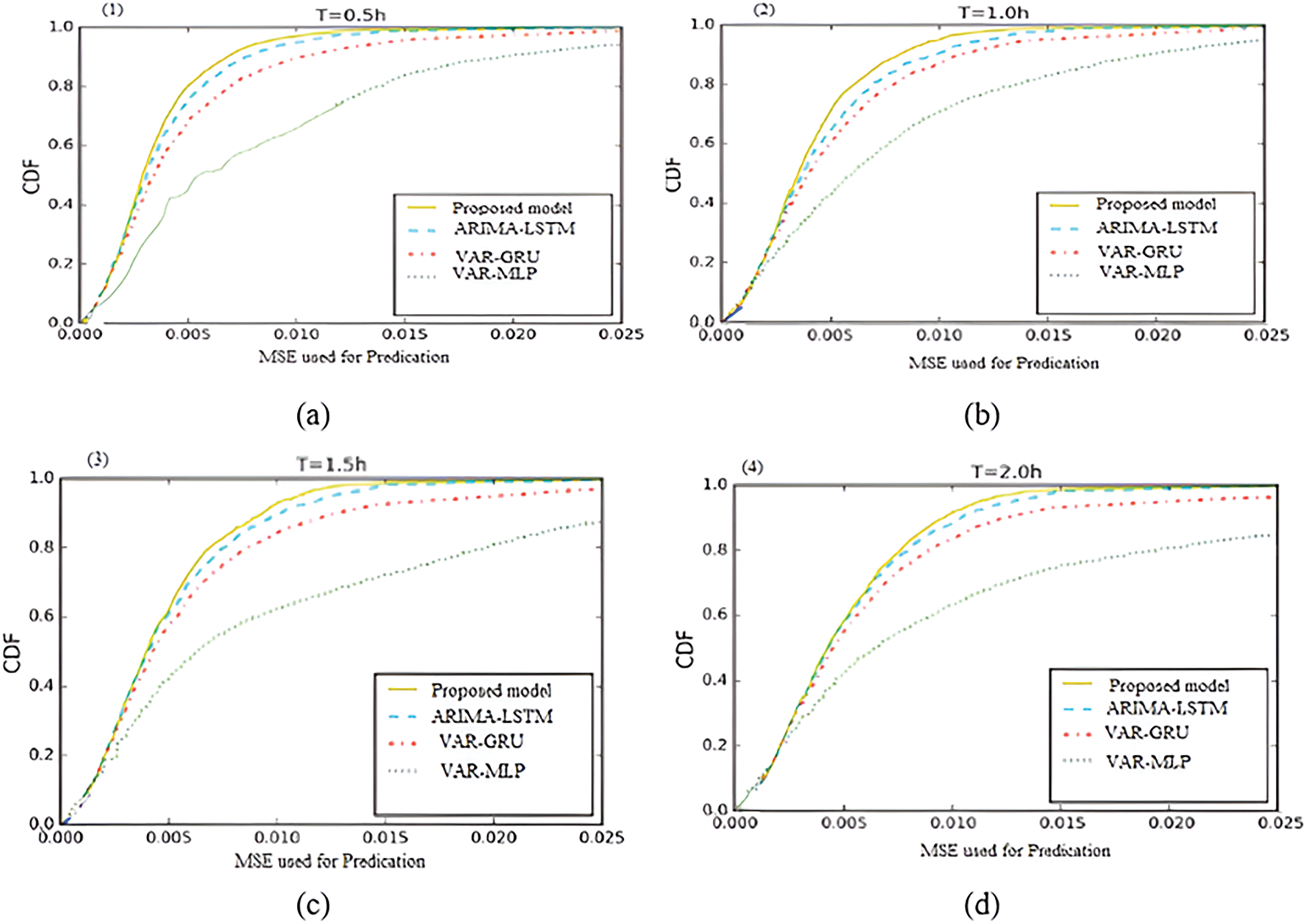
Figure 4: Prediction results based on different models
Improving resource usage in cloud data centers requires precise forecasting of CPU and RM utilization. The accuracy of the prediction outcomes for this method was assessed using mean-squared error (MSE), which is defined in Eq. (17).
where yi is the actual or real load value, ŷi is the anticipated load value at time value i, and n is the prediction length. Due to the straightforward, regular changes shown in Fig. 4, our suggested model is able to produce an accurate prediction with historical values. Following the simulation, two types of results are obtained: a specific result and an overall result.
The cumulative distribution function (CDF) of MSE for several models is displayed in Fig. 4a–d. The Google load trace interval is 5 min, and the steps ahead where a T = 0.5 h are up to 2 h. T = 1.0 h for (b). Based on the data from Fig. 4c, T = 1.5 h and (d) T = 2.0 h, our suggested model predicts better results than the other models.
4.4 Load Trace Distribution on the System
The time services chosen here originated from the four most interesting host loads—Axp0, AXP7, Sahara, and Themis—that were collected from load traces on Unix systems by [49]. We employed an HPC system to forecast load traces. Table 4 illustrates these four load traces’ varieties in terms of capture times and machine types, in addition to other aspects. After the load trace was scaled to a range of (0,1,0, 9), each load trace was normalized using the previously described algorithm. Eq. (18) presents the upper bound and lower bound, respectively, of each load trace’s maximum and minimum values. Fig. 5 displays the outcome of one of the traces.
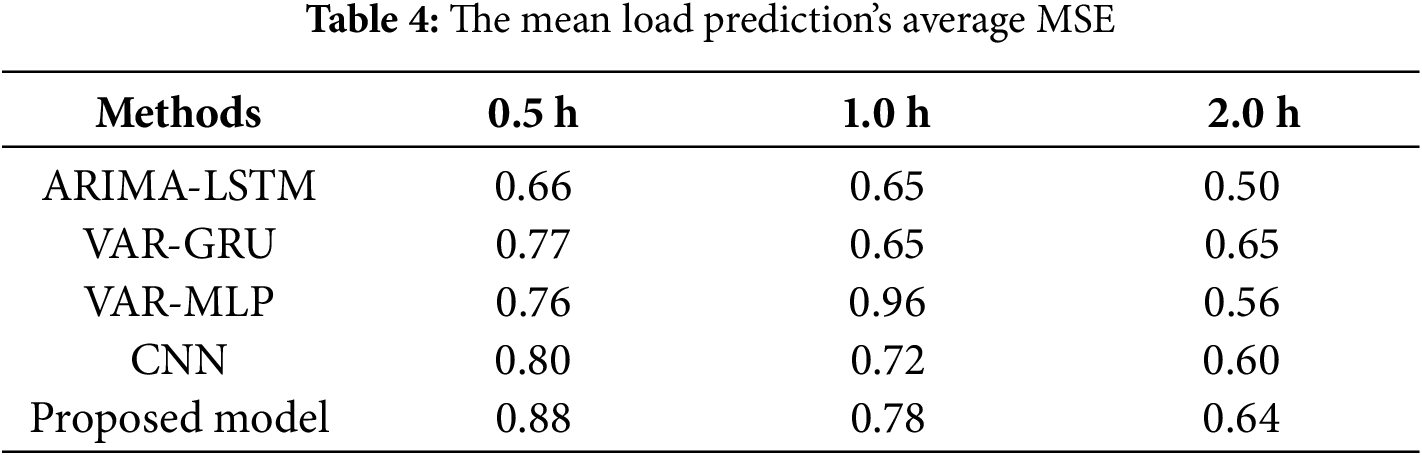
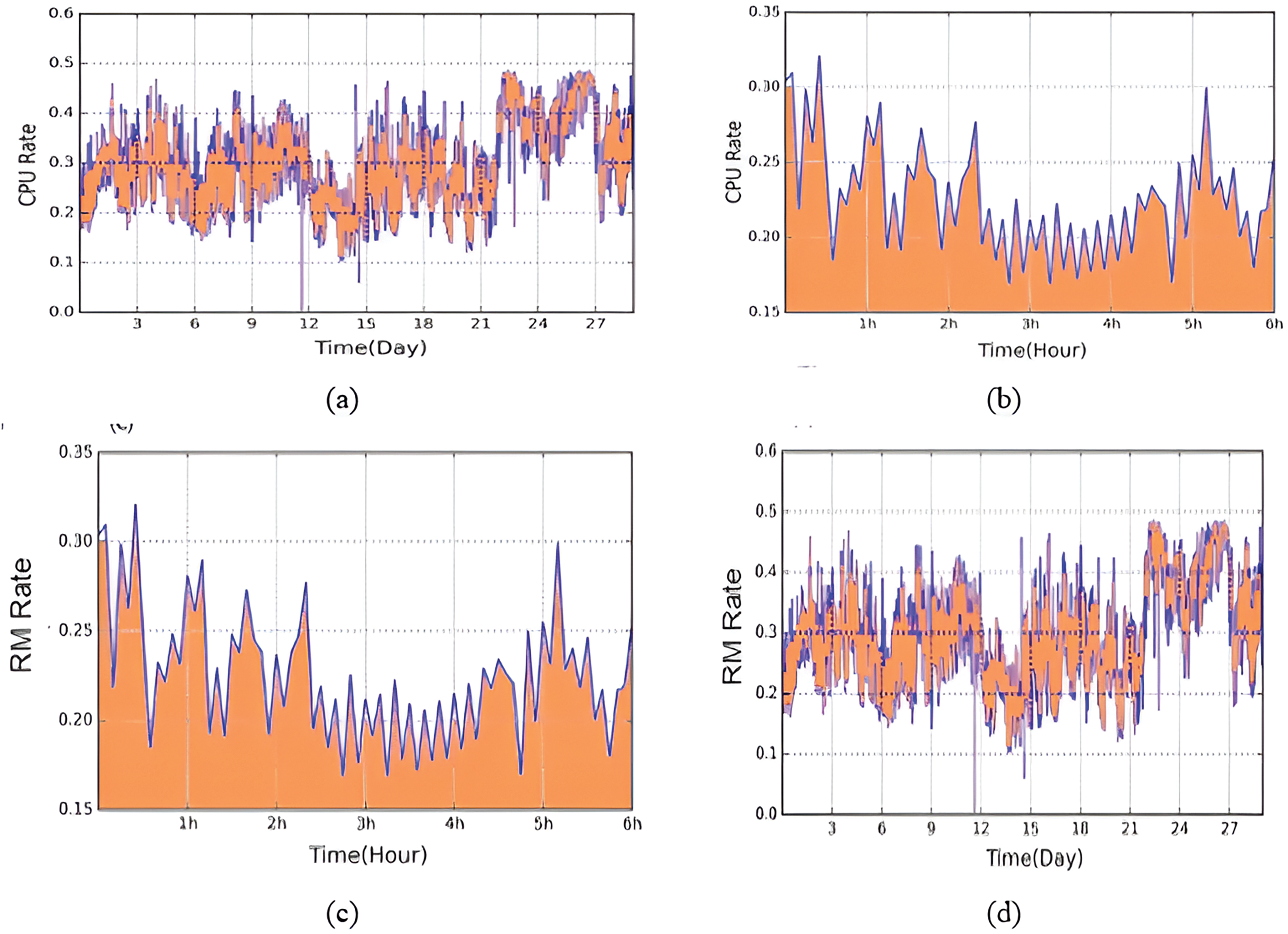
Figure 5: Normalized load trace system
The normalized axp7 load trace in Fig. 5 refers to two distinct load traces: the entire load trace and the axp7 load trace. These are further described in the trace’s Fig. 5b,c and Fig. 5a,d sections. If each load trace has a length of 1,200,000 and a b length of 200, and the highest and minimum values are denoted by the variables xmax and xmin, respectively. UPB is the upper bound and LWB is the lower bound.
An essential part of improving the cloud computing resource allocation system is predicting host load. Because data centers vary more than ever, cloud systems require accurate prediction. Because of this, two actual load traces were used in this paper’s assessment of the performance. The initial is one load traced in the Google data center, and the other in a conventional distributed system. The experiment results show that our proposed method achieves higher accuracy and state-of-the-art performance in both datasets. By comparing our suggested model with the other four models only based on projected real load levels, we assess each model’s capacity to generate data by giving it the original Google cluster dataset hyper-parameters. Each load trace had 80% of its duration devoted to training and the remaining portion devoted to testing for the purposes of this study. The prediction findings are listed in Figs. 6 and 7. The proposed model proposes strong generation based on execution and time based on such facts.
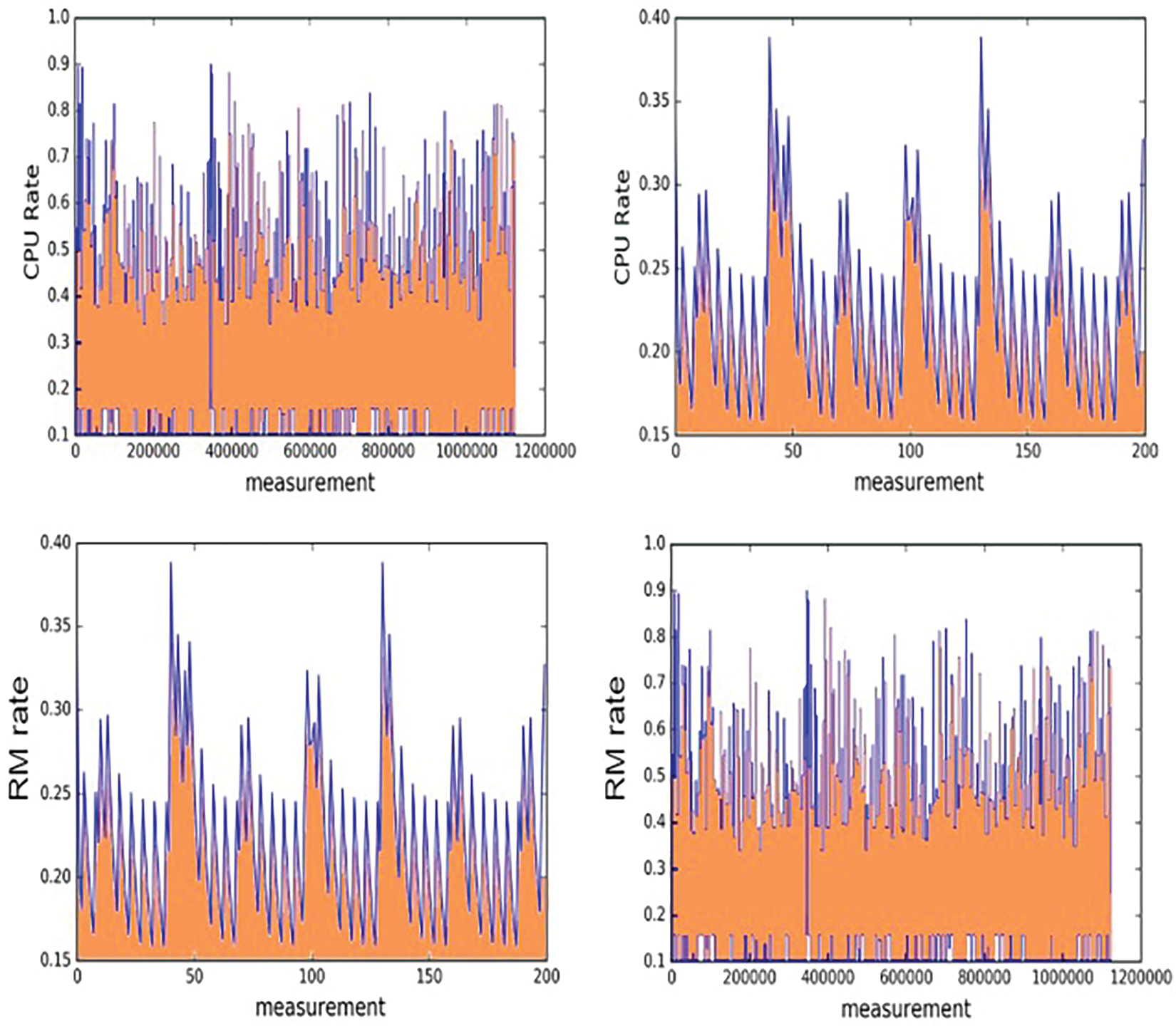
Figure 6: Predication results of RM
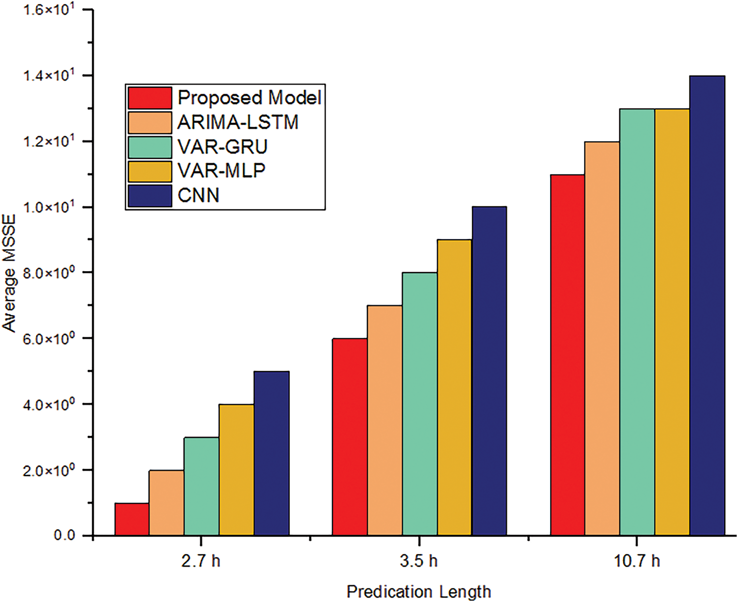
Figure 7: Overall predication result of different algorithms
The actual load forecast findings are mentioned in Left, together with the two load projections from Figs. 6 and 7. the Unix platforms listed in Right for the axp7 load traces. Sharp swings are seen in the noisy load trace of the Google cluster data. These findings show that the performance of our proposed model is essentially satisfactory.
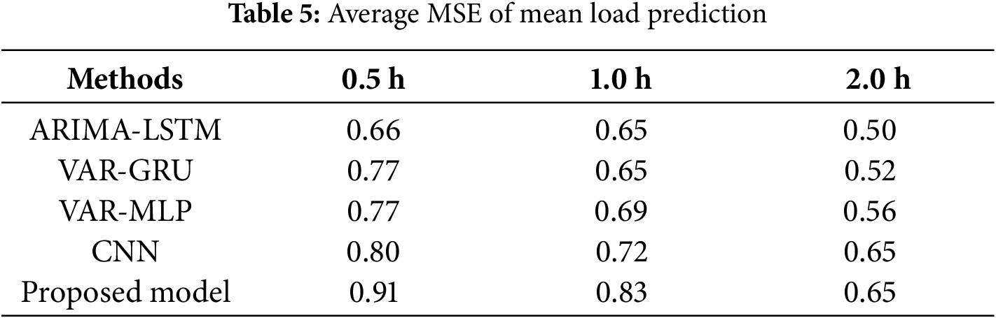
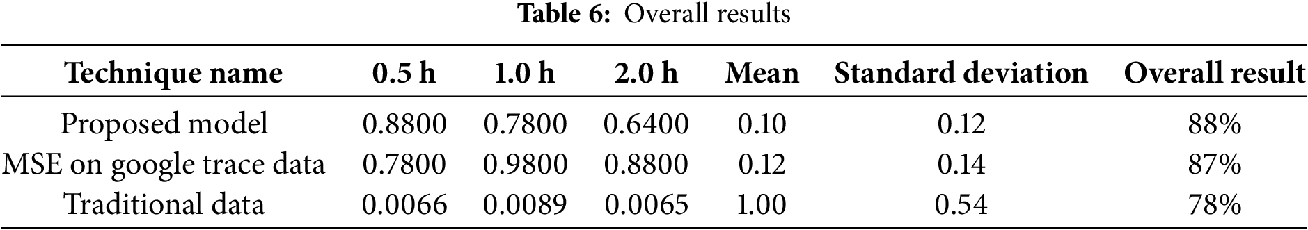
The MSE load prediction results are shown in Table 4. Our suggested model outperforms existing models in terms of accuracy, as evidenced by the findings, which show an increase of 88.78% in mean load prediction 0.5 h ahead of time, 78.06% in 0.5 h, and 64.71% in 1 h, respectively. 91% of the mean load estimate made 0.5 h in advance was accurate, 83% in 0.5 h, and 65% in 1 h. The results of traditional data are displayed in Table 5, where the recommended approach yields an efficient outcome when compared to alternative methods. Table 6 displays the outcome.
Overall, the proposed CNN-LSTM-VAR hybrid model outperforms traditional models like ARIMA and MLP in handling non-linear, irregular patterns, capturing long-term dependencies, and achieving higher accuracy with lower prediction errors. While it is computationally more demanding, its advantages in adaptability, generalization, and robustness make it well-suited for complex time series forecasting tasks, such as virtual machine (VM) or CPU utilization prediction.
5 Contributions of the Proposed Model
Giving consumers access to virtual computing resources including networking, storage, and hardware, the infrastructure service model offers adaptable, scalable, and reasonably priced solutions. It enables on-demand resource access, improving scaling, cutting down on operational costs, and optimizing resource consumption. Host load prediction maximizes cost, efficiency, and performance by better allocating cloud resources. Response times are impacted by issues like virtual machine migration and over-subscription, but prediction algorithms can help by predicting resource consumption, reducing latency, and improving system performance. Dynamic scalability modifies resources in response to demand, preserving the quality of the service. By integrating these capabilities, the proposed model supports dynamic cloud scalability with an advanced level of service quality, optimizing resource allocation for both cost-efficiency and performance reliability. Moreover, detecting spatial and temporal data patterns, CNNs and LSTMs enhance cloud resource analysis and forecasting, while vector auto-regression models forecast resource requirements based on historical usage. When combined, these methods enhance service quality, performance, and resource efficiency in cloud infrastructures.
By fusing CNN’s spatial-temporal feature extraction with LSTM’s long-term memory retention and VAR’s capacity to manage linear relationships, the suggested CNN-LSTM-VAR hybrid model overcomes the drawbacks of conventional methods. The model can learn intricate patterns, adjust to non-linear dependencies, and enhance prediction accuracy and generalization thanks to its integration. CNNs bring valuable insights into VM and CPU utilization by extracting intricate spatial-temporal patterns, enabling efficient anomaly detection, capturing both granular and long-term trends, and supporting adaptive and scalable analysis. These capabilities make CNNs powerful tools for optimizing virtualized environments and enhancing the performance of cloud infrastructure.
Using VAR as a preprocessing step or as a complementary component in the hybrid CNN-LSTM model improves its ability to capture both linear and non-linear dependencies in time-series data. This combination can ultimately lead to more accurate predictions, lower error rates, and better generalization to unseen data. By improving the learning of non-linear correlations, decreasing convergence time, and boosting robustness, filtering data to eliminate linear interdependencies further maximizes model performance. It allows CNN-LSTM models to concentrate on learning non-linear, intricate patterns, leading to improved generalization, faster convergence, and overall better model performance. This preprocessing step helps ensure that each layer is used to its full potential, contributing to a more robust and efficient hybrid model.
Additionally, using a scaled polynomial constant activation function, dead neurons are avoided which enhances consistency across layers. The function provides stability in gradient flow across CNN and LSTM layers and makes handling varying data scales more flexible. These advantages make the scaled polynomial constant activation function particularly well-suited for handling the complex dependencies and feature hierarchies involved in tasks like resource utilization analysis, anomaly detection, and predictive maintenance in VM and CPU data monitoring.
Moreover, Extended Short-Term Memory (E-STM) networks are particularly advantageous for time series data with irregular trends due to their adaptive memory retention, dynamic time step handling, resilience to irregular sampling and missing values and capability to capture both short-term and long-term dependencies. These features make E-STMs especially useful for cloud host utilization predication where trends are unpredictable and vary over time. In this proposed model, the E-STM improves the model’s attention to important events while controlling multi-scale temporal dynamics, which makes it perfect for applications with erratic patterns, such as predictive maintenance and anomaly detection.
One important aspect of cloud computing was allocating resources and apps based on actual consumption. However, the process of allocating resources required a setup time. This implied that planning would be necessary in order to predict the quantity of resources required in the future. In this work, we therefore introduced a novel host prediction technique that incorporates CPU utilization prediction with RM. The hybrid CNN-LSTM model for multivariate workload prediction was just released. Complex features were extracted from the CPU and virtual machine utilization components with the help of this enabled feature. This method made use of the temporal knowledge of irregular tendencies in the time series components. Using two different test types based on dataset results, we additionally assessed our proposed model. The suggested method performed well in both datasets. Our recommended approach produced successful outcomes in both preprocess and post-process conditions when compared to earlier models. However, in order to lower data center costs and increase resource efficiency using various dataset kinds in the actual cloud computing environment, the proposed method had to be integrated into the scheduling algorithm. The proposed algorithm design may be further improved by implementing automated search techniques for tuning hyperparameters, compressing the model to enable low-resource devices implementation or incorporating explainability models such as SHAP and LIME to improve understanding on the predictions made by the proposed model.
Acknowledgement: Not applicable.
Funding Statement: The article processing fee charges was funded by Multimedia University (Ref: MMU/RMC/PostDoc /NEW/2024/9804).
Author Contributions: Arif Ullah contributed to the conceptualization, research methodology and developed the initial proposed model. Siti Fatimah Abdul Razak contributed to the literature review, critically analyzing the reviewed articles and contributed to the overall structure and final editing of the manuscript. Sumendra Yogarayan and Md Shohel Sayeed provide the technical modifications and improvements of the proposed model. All authors reviewed the results and approved the final version of the manuscript.
Availability of Data and Materials: Due to university policy, supporting data is not available.
Ethics Approval: Not applicable.
Conflicts of Interest: The authors declare no conflicts of interest to report regarding the present study.
Abbreviations
| IaaS | Infrastructure as Services |
| IoT | Internet of Thing |
| SaaS | Software as a Service |
| VM | Virtual Machine |
References
1. Zheng Z, Zhang B, Liu Y, Ren J, Zhao X, Wang Q. An approach for predicting multiple-type overflow vulnerabilities based on combination features and a time series neural network algorithm. Comput Secur. 2022;114(7):102572. doi:10.1016/j.cose.2021.102572. [Google Scholar] [CrossRef]
2. He Z, Chen P, Li X, Wang Y, Yu G, Chen C, et al. A spatiotemporal deep learning approach for unsupervised anomaly detection in cloud systems. IEEE Trans Neural Netw Learn Syst. 2023;34(4):1705–19. doi:10.1109/TNNLS.2020.3027736. [Google Scholar] [PubMed] [CrossRef]
3. Zhang Y, Liu B, Gong Y, Huang J, Xu J, Wan W. Application of machine learning optimization in cloud computing resource scheduling and management. In: Proceedings of the 5th International Conference on Computer Information and Big Data Applications; 2024; Wuhan, China; ACM. p. 171–5. doi:10.1145/3671151.3671183. [Google Scholar] [CrossRef]
4. Wu Y, Yuan Y, Yang G, Zheng W. Load prediction using hybrid model for computational grid. In: 2007 8th IEEE/ACM International Conference on Grid Computing; 2007 Sept 19–21. Austin, TX, USA: IEEE; 2007. p. 235–42. doi:10.1109/GRID.2007.4354138. [Google Scholar] [CrossRef]
5. Wang Y, Zhang Y, Wu Z, Li H, Christofides PD. Operational trend prediction and classification for chemical processes: a novel convolutional neural network method based on symbolic hierarchical clustering. Chem Eng Sci. 2020;225:115796. doi:10.1016/j.ces.2020.115796. [Google Scholar] [CrossRef]
6. Lu Y, Phillips GM, Yang J. The impact of cloud computing and AI on industry dynamics and competition. Educat Administrat: The Pract. 2024;30(7):797–804. doi:10.53555/kuey.v30i7.6851. [Google Scholar] [CrossRef]
7. Bengio Y, Simard P, Frasconi P. Learning long-term dependencies with gradient descent is difficult. IEEE Trans Neural Netw. 1994;5(2):157–66. doi:10.1109/72.279181. [Google Scholar] [PubMed] [CrossRef]
8. Fang W, Zhang F, Ding Y, Sheng J. A new sequential image prediction method based on LSTM and DCGAN. Comput Mater Contin. 2020;64(1):217–31. doi:10.32604/cmc.2020.06395. [Google Scholar] [CrossRef]
9. Simaiya S, Lilhore UK, Sharma YK, Rao KBVB, Maheswara Rao VVR, Baliyan A, et al. A hybrid cloud load balancing and host utilization prediction method using deep learning and optimization techniques. Sci Rep. 2024;14(1):1337. doi:10.1038/s41598-024-51466-0. [Google Scholar] [PubMed] [CrossRef]
10. Dittakavi RSS. Deep learning-based prediction of CPU and memory consumption for cost-efficient cloud resource allocation. Sage Science Rev Appl Mach Lear. 2021;4(1):45–58. [Google Scholar]
11. Ouhame S, Hadi Y, Ullah A. An efficient forecasting approach for resource utilization in cloud data center using CNN-LSTM model. Neural Comput Appl. 2021;33(16):10043–55. doi:10.1007/s00521-021-05770-9. [Google Scholar] [CrossRef]
12. Rawat PS, Kushwaha JP. Reliable resource optimization model for cloud using adversarial neural network. In: Advanced computing techniques for optimization in cloud. Boca Raton, FL, USA: Chapman and Hall/CRC eBooks; 2024. p. 124–49. [Google Scholar]
13. Damaševičius R, Sidekerskienė T. Short time prediction of cloud server round-trip time using a hybrid neuro-fuzzy network. J Artif Intell Syst. 2020;2(1):133–48. doi:10.33969/AIS.2020.21009. [Google Scholar] [CrossRef]
14. Kholidy HA. An intelligent swarm based prediction approach for predicting cloud computing user resource needs. Comput Commun. 2020;151(1):133–44. doi:10.1016/j.comcom.2019.12.028. [Google Scholar] [CrossRef]
15. Ralha CG, Mendes AHD, Laranjeira LA, Araújo APF, Melo ACMA. Multiagent system for dynamic resource provisioning in cloud computing platforms. Future Gener Comput Syst. 2019;94(2):80–96. doi:10.1016/j.future.2018.09.050. [Google Scholar] [CrossRef]
16. Zhu Y, Zhang W, Chen Y, Gao H. A novel approach to workload prediction using attention-based LSTM encoder-decoder network in cloud environment. EURASIP J Wirel Commun Netw. 2019;2019(1):274. doi:10.1186/s13638-019-1605-z. [Google Scholar] [CrossRef]
17. Biswas NK, Banerjee S, Biswas U, Ghosh U. An approach towards development of new linear regression prediction model for reduced energy consumption and SLA violation in the domain of green cloud computing. Sustain Energy Technol Assess. 2021;45(4):101087. doi:10.1016/j.seta.2021.101087. [Google Scholar] [CrossRef]
18. Jyoti A, Shrimali M, Tiwari S, Singh HP. Cloud computing using load balancing and service broker policy for IT service: a taxonomy and survey. J Ambient Intell Humaniz Comput. 2020;11(11):4785–814. doi:10.1007/s12652-020-01747-z. [Google Scholar] [CrossRef]
19. Huang H, Wang Y, Cai Y, Wang H. A novel approach for energy consumption management in cloud centers based on adaptive fuzzy neural systems. Clust Comput. 2024;27(10):14515–38. doi:10.1007/s10586-024-04665-3. [Google Scholar] [CrossRef]
20. de Lima EC, Rossi FD, Luizelli MC, Calheiros RN, Lorenzon AF. A neural network framework for optimizing parallel computing in cloud servers. J Syst Archit. 2024;150:103131. doi:10.1016/j.sysarc.2024.103131. [Google Scholar] [CrossRef]
21. Abdullah L, Li H, Al-Jamali S, Al-Badwi A, Ruan C. Predicting multi-attribute host resource utilization using support vector regression technique. IEEE Access. 2020;8:66048–67. doi:10.1109/ACCESS.2020.2984056. [Google Scholar] [CrossRef]
22. Baig SUR, Iqbal W, Berral JL, Carrera D. Adaptive sliding windows for improved estimation of data center resource utilization. Future Gener Comput Syst. 2020;104(2):212–24. doi:10.1016/j.future.2019.10.026. [Google Scholar] [CrossRef]
23. Gamal M, Rizk R, Mahdi H, Elnaghi BE. Osmotic bio-inspired load balancing algorithm in cloud computing. IEEE Access. 2019;7:42735–44. doi:10.1109/ACCESS.2019.2907615. [Google Scholar] [CrossRef]
24. Bilski J, Smoląg J, Kowalczyk B, Grzanek K, Izonin I. Fast computational approach to the levenberg-marquardt algorithm for training feedforward neural networks. J Artif Intell Soft Comput Res. 2023;13(2):45–61. doi:10.2478/jaiscr-2023-0006. [Google Scholar] [CrossRef]
25. Javadpour A, Sangaiah AK, Pinto P, Ja’fari F, Zhang W, Majed Hossein Abadi A, et al. An Energy-optimized Embedded load balancing using DVFS computing in Cloud Data centers. Comput Commun. 2023;197(3):255–66. doi:10.1016/j.comcom.2022.10.019. [Google Scholar] [CrossRef]
26. Abdullah M, Khana S, Alenezi M, Almustafa K, Iqbal W. Application centric virtual machine placements to minimize bandwidth utilization in datacenters. Intell Autom Soft Comput. 2020;26(1):13–25. doi:10.31209/2018.100000047. [Google Scholar] [CrossRef]
27. Javadpour A, Nafei A, Ja’fari F, Pinto P, Zhang W, Sangaiah AK. An intelligent energy-efficient approach for managing IoE tasks in cloud platforms. J Ambient Intell Humaniz Comput. 2023;14(4):3963–79. doi:10.1007/s12652-022-04464-x. [Google Scholar] [CrossRef]
28. Thakkar HK, Dehury CK, Sahoo PK. MUVINE: multi-stage virtual network embedding in cloud data centers using reinforcement learning-based predictions. IEEE J Sel Areas Commun. 2020;38(6):1058–74. doi:10.1109/JSAC.2020.2986663. [Google Scholar] [CrossRef]
29. Saxena D, Singh AK, Buyya R. OP-MLB: an online VM prediction-based multi-objective load balancing framework for resource management at cloud data center. IEEE Trans Cloud Comput. 2022;10(4):2804–16. doi:10.1109/TCC.2021.3059096. [Google Scholar] [CrossRef]
30. Raza B, Aslam A, Sher A, Malik AK, Faheem M. Autonomic performance prediction framework for data warehouse queries using lazy learning approach. Appl Soft Comput. 2020;91(7):106216. doi:10.1016/j.asoc.2020.106216. [Google Scholar] [CrossRef]
31. Ullah A, Alam T, Aziza C, Sebai D, Abualigah L. A hybrid strategy for reduction in time consumption for cloud datacenter using HMBC algorithm. Wirel Pers Commun. 2024;137(4):2037–60. doi:10.1007/s11277-024-11395-7. [Google Scholar] [CrossRef]
32. Bawa S, Rana PS, Tekchandani R. Multivariate time series ensemble model for load prediction on hosts using anomaly detection techniques. Clust Comput. 2024;27(8):10993–1016. doi:10.1007/s10586-024-04517-0. [Google Scholar] [CrossRef]
33. Dinesh Kumar K, Umamaheswari E. An efficient proactive VM consolidation technique with improved LSTM network in a cloud environment. Computing. 2024;106(1):1–28. doi:10.1007/s00607-023-01214-5. [Google Scholar] [CrossRef]
34. Ullah A, Nawi NM, Uddin J, Baseer S, Rashed AH. Artificial bee colony algorithm used for load balancing in cloud computing. IAES Int J Artif Intell. 2019;8(2):156. doi:10.11591/ijai.v8.i2.pp156-167. [Google Scholar] [CrossRef]
35. Ullah A, Nawi NM. An improved in tasks allocation system for virtual machines in cloud computing using HBAC algorithm. J Ambient Intell Humaniz Comput. 2023;14(4):3713–26. doi:10.1007/s12652-021-03496-z. [Google Scholar] [CrossRef]
36. Sunyaev A. Cloud computing. In: Internet computing: principles of distributed systems and emerging internet-based technologies. Cham: Springer; 2024. p. 165–209. doi:10.1007/978-3-031-61014-1_6. [Google Scholar] [CrossRef]
37. Yanamala AKY. Optimizing data storage in cloud computing: techniques and best practices. Int J Adv Eng Technol Innovat. 2024;1(3):476–513. doi:10.53555/nveo.v8i3.5760. [Google Scholar] [CrossRef]
38. Ghandour O, El Kafhali S, Hanini M. Computing resources scalability performance analysis in cloud computing data center. J Grid Comput. 2023;21(4):61. doi:10.1007/s10723-023-09696-5. [Google Scholar] [CrossRef]
39. Mushtaq MF, Akram U, Khan I, Khan SN, Shahzad A, Ullah A. Cloud computing environment and security challenges: a review. Int J Adv Comput Sci Appl. 2017;8(10):183–95. doi:10.14569/ijacsa.2017.081025. [Google Scholar] [CrossRef]
40. Umar S, Baseer S, Arifullah. Perception of cloud computing in universities of Peshawar, Pakistan. In: 2016 Sixth International Conference on Innovative Computing Technology (INTECH); 2016 Aug 24–26. Dublin, Ireland: IEEE; 2016. p. 87–91. doi:10.1109/INTECH.2016.7845046. [Google Scholar] [CrossRef]
41. Ouhame S, Hadi Y, Arifullah A. A hybrid grey wolf optimizer and artificial bee colony algorithm used for improvement in resource allocation system for cloud technology. Int J Onl Eng. 2020;16(14):4–17. doi:10.3991/ijoe.v16i14.16623. [Google Scholar] [CrossRef]
42. Ammavasai SK. Dynamic task scheduling in edge cloud systems using deep recurrent neural networks and environment learning approaches. J Intell Fuzzy Syst. 2024;2024(4):1–16. doi:10.3233/JIFS-236838. [Google Scholar] [CrossRef]
43. Aarthi E, Sheela MS, Vasantharaj A, Saravanan T, Rama RS, Sujaritha M. Integrating neural network-driven customization, scalability, and cloud computing for enhanced accuracy and responsiveness for social network modelling. Soc Netw Anal Min. 2024;14(1):139. doi:10.1007/s13278-024-01302-0. [Google Scholar] [CrossRef]
44. Sabyasachi AS, Sahoo BM, Ranganath A. Deep CNN and LSTM approaches for efficient workload prediction in cloud environment. Procedia Comput Sci. 2024;235(2):2651–61. doi:10.1016/j.procs.2024.04.250. [Google Scholar] [CrossRef]
45. Sujatha D, Raj TFM, Ramesh G, Agoramoorthy M, Ali SA. Neural networks-based predictive models for self-healing in cloud computing environments. In: 2024 International Conference on Intelligent and Innovative Technologies in Computing, Electrical and Electronics (IITCEE); 2024 Jan 24–25. Bangalore, India: IEEE; 2024. p. 1–4. doi:10.1109/IITCEE59897.2024.10467499 [Google Scholar] [CrossRef]
46. Kisel'ák J, Lu Y, Švihra J, Szépe P, Stehlík M. “SPOCU”: scaled polynomial constant unit activation function. Neural Comput Appl. 2021;33(8):3385–401. doi:10.1007/s00521-020-05182-1. [Google Scholar] [CrossRef]
47. Tandon A, Patel S. DBSCAN based approach for energy efficient VM placement using medium level CPU utilization. Sustain Comput Inform Syst. 2024;43(4):101025. doi:10.1016/j.suscom.2024.101025. [Google Scholar] [CrossRef]
48. Gurusamy S, Selvaraj R. Resource allocation with efficient task scheduling in cloud computing using hierarchical auto-associative polynomial convolutional neural network. Expert Syst Appl. 2024;249(6):123554. doi:10.1016/j.eswa.2024.123554. [Google Scholar] [CrossRef]
49. Kirchoff DF, Meyer V, Calheiros RN, De Rose CAF. Evaluating machine learning prediction techniques and their impact on proactive resource provisioning for cloud environments. J Supercomput. 2024;80(15):21920–51. doi:10.1007/s11227-024-06303-6. [Google Scholar] [CrossRef]
Cite This Article
 Copyright © 2025 The Author(s). Published by Tech Science Press.
This work is licensed under a Creative Commons Attribution 4.0 International License , which permits unrestricted use, distribution, and reproduction in any medium, provided the original work is properly cited.
 Downloads
 Citation Tools