Semi-Supervised Medical Image Classification Based on Sample Intrinsic Similarity Using Canonical Correlation Analysis

1  Introduction

Recently, image processing has made remarkable achievements, such as image segmentation [1], image recognition [2], and especially in medical image classification [3]. Usually, good performance is closely correlated with the quality of samples. However, clinical physicians find it challenging to collect maker samples, as annotating medical images requires extensive expertise and work. Many academics have begun to use unsupervised learning [4], semi-supervised learning [5], and weakly supervised learning [6] rather than traditional supervised learning since it is easier for researchers to collect unlabeled clinical images.

Semi-supervised learning has been shown to perform better when labeled data is limited. Nowadays, most semi-supervised medical image analyses are based on consistent regular strategies [7,8], which regularize the outputs of networks to utilize unlabeled data fully. These methods feed the same images under different noises into the networks and force prediction results to be as similar as possible. Given some examples, the Temporal Ensembling (TE) model [7] applies exponential moving average (EMA) predictions for unlabeled data as consistency targets. Mean-teacher (MT) [8] was introduced based on the TE model, where teacher network outputs could serve as reliable consistency targets. However, both TE and MT primarily focus on the consistency of reliable targets. As a result, numerous features of unlabeled images are not fully exploited.

As for skin lesion classification, many works [9] have been conducted. Earlier computer-aided diagnosis (CAD) for skin lesion classification heavily relied on manual characteristics extraction and subsequently put these features into networks. Obviously, this approach is very inefficient. Therefore, many scholars are beginning to utilize convolutional neural networks (CNN) to boost the productivity of classification. Rahmouni et al. [10] developed a novel framework based on self-attention which can overcome the complexity of the skin dataset. Deep residual networks proposed by Yu et al. [11] could determine whether the input data is a melanoma sample. Despite these studies having achieved promising results, all of them ignore the imbalanced problem of the skin dataset.

In this paper, we offer a new algorithm based on a consistency-based strategy, making the most of the limited labeled samples. We introduce a correlation loss to unsupervised loss by modeling features relation with Canonical Correlation Analysis (CCA) [12]. Moreover, we propose to improve the supervised loss to address the class imbalance issue so that the accuracy of medical categorization can be significantly increased. Lastly, we evaluate our method using ISIC 2017 [13] and ISIC 2018 [14].

The contributions are summarized in three points:

1. We introduce a feature consistency paradigm, fully extracting the information of unlabeled images by introducing a correlation loss with CCA enforcing feature relation;

2. We address the problem of uneven data distribution as much as possible by improving supervised loss;

3. We evaluate our model on ISIC 2017 and ISIC 2018, showing that our model could perform better compared to other state-of-the-art semi-supervised methods. Additionally, we demonstrate that our method is more outstanding than other models by conducting extensive ablation studies.

2  Related Work

2.1 Consistency Enforcing Strategy

Consistent regular learning could leverage valuable information from massive unlabeled images. TE model utilizes EMA to update the parameters once in every epoch, and then the purpose of improving the quality of the consistency target is achieved to a certain extent. However, the TE model introduces new hyperparameters, making it heavy while updating the predictions. To address the shortcomings of the TE model, the MT model was proposed. MT model includes two networks: teacher network and student network. The model updates hyperparameters of the teacher model using EMA from the student model, enabling the teacher network to generate reliable consistency targets. Based on these models, numerous researchers have begun to commit to researching how to produce reliable consistency targets. For example, Xie et al. [15] presented the MK-SSAC model, which demonstrated that leveraging improved image enhancement techniques can yield better classification results. A new loss called Certainty-driven Consistency loss was put forward by Liu et al. [16] to improve the quality of the teacher targets, enabling the student model to gain knowledge dynamically from high-reliability consistency targets. In contrast to the studies mentioned above, we aim to enhance the performance of traditional consistency regularization models by paying more attention to the intrinsic relationships between samples.

2.2 Canonical Correlation Analysis

CCA is a statistical method that finds linear combinations of two random variables. In medical analysis, CCA is generally used in feature fusion and brain imaging genetics. For example, Zhou et al. [17] proposed a model called F-CCA, which could reduce unfairness by minimizing the correlation disparity error connected with protected attributes. Moreover, numerous CCA extension methods are emerging. Andrew et al. [18] proposed DCCA (Deep Canonical Correlation Analysis), which is designed to be suitable for DNN training using mini-batches. SCCA (Sparse Canonical Correlation Analysis) has become increasingly popular in imaging genetics [19] research due to its powerful capabilities in discovering bi-multivariate relationships and capturing features. For instance, Zhang et al. [20] introduced the MTCDA model to study brain imaging genetics and identify the specificity of disease. It can be seen that CCA has already been widely applied to medical analysis. However, SCCA and DCCA both have some drawbacks. DCCA requires massive marker samples, which are often rare, and there are certain risks of overfitting while using DCCA. SCCA typically demands more computational resources and training time to maintain the sparsity of the correlation model. Therefore, we think that we can also try to apply CCA to the Teacher-Student network. Here, we first extract the student and teacher features just before the last pooling layer, and then use CCA to measure the similarity between these features. In this way, we can focus on the features that are crucial in classification tasks.

2.3 Supervised Loss

Considering the imbalanced skin datasets, it is not a wise choice to utilize cross-entropy loss [21] as the supervised loss in our framework. Because cross-entropy loss would lead the model to be more inclined to learn from the class with more samples, resulting in worse performance in classes with fewer samples. Multiple balancing methods [22] are frequently considered, where the loss weighting is set as , and is the category number. A novel loss called Class-Balanced Loss [23] was designed by Cui et al., where and the parameter . These approaches can largely address the issue of rational loss weighting allocation in cross-entropy loss. However, these methods limited the range of variation in loss weighting (i.e., from 1 to ). Consequently, Yao et al. proposed a new loss called Multi-Weighted New Loss (MWNL) [9], which extended the scope of loss weighting and adapted the training epoch.

2.4 The Method of Sample Relation

In previous work, most studies focused on enhancing the quality of consistent predictions, ignoring the intrinsic relationships between features. Taking inspiration from the recent study on graph neural network [24], we can get more useful information if we exploit the correlation between different samples. Liu et al. [25] proposed a relation-driven model called SRC-MT, which utilizes a Gram Matrix [26] to look for similarities between samples. In this framework, a small batch with B samples was given, from which the feature map of layer l was obtained. The feature graph is then reshaped into , where H and W denote the dimensions of the feature map, and C represents the number of channels. The similarity between samples was computed by the following formula:

(1)

To normalize the Gram matrix, the final relation matrix is defined as:

(2)

The SRC-MT model encouraged the network to learn more useful information from unlabeled inputs. However, the Gram Matrix may lose some characteristic information because of its multiplication relation and the reduction of dimensions. Hence, we offer to explore the similarity between sample features by utilizing CCA.

3  Method

3.1 The Backbone of CSRC

Fig. 1 depicts our proposed semi-supervised framework, which reflects the novelty of our paper. Our semi-supervised framework follows the consistency principle and updates the network using three loss components: correlation loss , balancing loss , and traditional consistency loss . This approach makes full use of the rich features carried by unlabeled data. Our framework introduces feature consistency based on traditional consistency regularization methods and addresses the data imbalance issue by improving the supervised loss. We describe the algorithm of our model with the following steps:

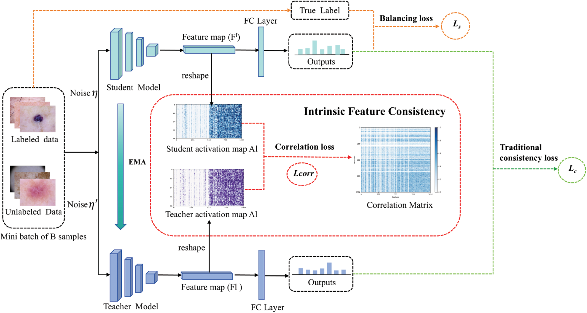
Figure 1: Overview of our framework

1. We defined the labeled data set as with N labeled samples and the unlabeled data set as , where is the input skin image, and is the human-annotated label. We optimize the network following Eq. (3). Where indicates supervised loss for addressing imbalanced classification, denotes unsupervised loss to enforce consistency by adding different perturbations. The target of our consistency-based framework is to train a classification network that can effectively leverage the information from unlabeled data.

(3)

2. Our consistency-based model fully explores the extra semantic information from unlabeled data by introducing a correlation loss to unsupervised loss. We processed the images and fed the same samples into the teacher-student network under different noise (usually Gaussian noise). Unlike traditional consistency models, we separately extract the features of the teacher and student networks during the feature extraction stage and then use CCA to enforce consistency between the features after the final pooling layer. During training, we encourage the model to explore the feature relation by minimizing the correlation loss .

3. Most semi-supervised models use the cross-entropy loss as the supervised loss to update the student network. However, cross-entropy loss may not be ideal for updating the network when the data distribution is imbalanced. To address the classification challenges posed by imbalanced data distribution, we improve the balancing loss , which is computed using true labels from labeled data and the student predictions.

4. Our model would preserve the traditional consistency loss , encouraging the consistency of teacher and student network predictions. This method emphasizes the consistency of network outputs under different noise. The consistency loss is defined as Eq. (4). Where and represent the different noises.

(4)

Here, we update the teacher network weights as EMA of student model . The iterative equation is defined as Eq. (5), and we set the EMA decay rate as 0.99, as recommended in the original paper.

(5)

3.2 Consistency of Intrinsic Features

As mentioned, traditional consistency regularization methods primarily focus on improving the consistency targets, while ignoring the relationships between features. Drawing inspiration from a previous study [24], we can gain more useful semantic information if we pay attention to the correlation between samples. Therefore, is used in our work, and this loss utilizes CCA to get extra useful knowledge from the unlabeled samples.

In our framework, a small batch with B samples is input, and the activation graph of layer l is denoted as . The feature map is then reshaped as , where and represent the spatial dimension of the feature graph, and C is the channel number. We standardize the feature matrix of the student model and the teacher model to obtain matrices and , i.e., Eq. (6).

(6)

We utilize CCA to explore the feature relation, and the is defined as Eq. (7). During the training process, we will continuously optimize so that the correlation between samples is greatest when it achieves a minimum. In Eq. (7), , , and respectively represent the covariance calculated by teacher activation and student activation, shown in Eq. (8). and respectively represent the left and right singular vector of the matrix . Finally, we can capture more semantic knowledge from unlabeled samples by minimizing Eq. (8).

(7)

(8)

3.3 Supervised Loss of Imbalanced Data

The original paper utilized the cross-entropy loss as the supervised loss. However, it is not a wise choice to use the cross-entropy loss, because it evenly distributes the loss weighting to each category of samples. This is a disadvantage for unbalanced datasets, as it would influence the model to gain useful knowledge from those with fewer samples and reduce the accuracy of model classification.

Recall from recent work [9], we could also rethink the supervised loss of our model from the aspects of loss-weighted and prediction threshold. Traditional balancing methods usually set the loss weighting to 1/N. However, we expand the range of loss weighting, enhancing the diversity of weighting strengths. As Eq. (9) shows, we combine the loss weighting with Focal loss, noticing samples with wrong classification. This approach helps reduce the sample imbalance between classes and alleviates the classification difficulty imbalance.

(9)

In Eq. (9), is the class weighting. For example, we could set a value greater than 1 while keeping the other class weighting as 1 to strengthen the training of class . represents the number of each sample. To extend the range of loss weighting, we add the hyperparameter . Clearly, the scope of loss weighting is extended beyond [1, 1/]. Then we make change with training epoch E to learn the deep features dynamically, as shown in Eq. (10). is the extension of Focal loss [27] defined by Eq. (11). As shown in Eq. (11), is the prediction probability defined as Eq. (12). Notably, , , Seriously affecting the optimization of network parameters. Therefore, we introduce a thread which can reduce the the interference of outliers .

(10)

(11)

(12)

Finally, we can define the total loss as Eq. (13). The total loss is composed of the supervised loss , consistency loss , and correlation loss . The role of is to balance supervised loss and unsupervised loss, and is updated by ; is a hyperparameter that finds a balance between consistency loss and correlation loss.

(13)

4  Experiments

We conduct experiments on ISIC 2017 and ISIC 2018. ISI C2017 is a skin dataset that has 2750 images, belonging to 3 categories. In our experiments, we split ISIC 2017 into training (2000), validation (150), and testing (600). ISIC 2018 is one of the largest and most used skin image datasets. This dataset comprises samples of 7 common skin diseases, with a total of 10,015 samples. The distribution of these two public datasets is shown in Table 1. Both of them suffer from the problem of data imbalance, so we could use them to conduct experiments.

4.1 Experimental Setup

During the training phase, a series of parameters have been set following the original paper [25], including: 1) Implementation of rotation, translation, and horizontal flips in each min batch. The rotation angle ranges from −10 to 10, pixels pan vertically and horizontally in the range of −2% to 2% of the width of the image. Additionally, there is a half-chance that the input sample will be randomly inverted. 2) We set the dropout rate to 0.2. Noteworthy, we only use the dropout layer in the stage of training but turn it off during the validation and testing stage. 3) We resize all samples to and normalize them using statistics from ImageNet [28]. For fairness, we randomly split ISIC 2018 into a training set, validation set, and test set with a ratio of 7:1:2, following SRC-MT. And we set the batch size to 48, containing 12 labeled data and 36 unlabeled data in each batch.

We improve our framework based on the SRCMT model [25] and use the densetnet121 as the backbone following the original model. At the time of training, the student network uses Adam optimizer [29] with initial learning (1e–4), and it decays at a power of 0.9 in each round. All the experiments are conducted on 1 NVIDIA GeForce GTX 3090 graphics using PyTorch.

4.2 Results and Analysis

To show the advancement of our model, we conduct experiments on extensive existing outstanding models (i.e., DermaDL [30], Self-training [31], DCGAN [32], MT [8], and SRC-MT [25]) on ISIC 2018. Specifically, DermaDL [30] is a semi-supervised model designed for skin lesion classification. Table 2 illustrates the different metric scores of diverse classification models with 20% marker skin samples. The upper bound performance is obtained as a baseline by training a supervised model using 100% labeled data, whereas the baseline is trained with only 20% labeled data. In Table 2, the specificity metric of self-training reaches 93.31%, indicating that this method can effectively identify negative samples. The SRC-MT obtains higher scores in all metrics than MT, indicating the importance of intrinsic features from samples. Meanwhile, our model achieves very high scores on most metrics than other methods, highlighting that our model indeed helps to explore the dark information of unlabeled data. In addition, we also choose different backbone networks such as Densenet161 and Resnet18 to conduct experiments. As shown in Table 2, we both improve the classification accuracy no matter we use which network as backbone. However, we get better achievements when we choose DenseNet as the backbone due to the introduction of dense blocks. Fig. 2 shows the AUC scores of each skin lesion of the three models (i.e., MT, SRC-MT, and our model) when using 20% labeled data. No matter what type of models we use, the AUC scores of almost all classes reach 90%, and the Vascular lesions even exceed 99%. However, the scores of Melanoma and Benign keratosis are relatively lower due to the lack of inter-class features. In addition, we can see that our model maintains the best AUC score in each category over other consistency-based methods, proving the advance of our framework.

Figure 2: AUC of each class on ISIC 2018

To examine the impact of varying amounts of labeled data, we conducted experiments with different numbers of labeled samples. In Fig. 3, we also visualize the AUC and Accuracy, in which the AUC and Accuracy performance of our model reaches 91% under most labeled data. From Table 3 and Fig. 3, we can see that, regardless of the proportion of labeled data used, our model consistently achieves higher scores than both the MT and SRC-MT models, highlighting the effectiveness of focusing on feature relations. However, when we use less labeled data (5% labeled data), the results will be slightly worse. This may be because there is too little labeled data to guarantee the reliability of the consistency target. In addition, in Fig. 4, we visualize the sensitivity of each under different labeled data. We can find that our model exhibits the most gradual changes as the data decreases, indicating the robustness of our model. This shows the good consistency and generalization of our CSRC algorithm.

Figure 3: The AUC and accuracy of our model with different labeled data

Figure 4: The sensitivity of each model with different labeled data

We also compare our model with the other two classic consistency-based methods (i.e., MT and SRC-MT) on ISIC 2017. Table 4 shows the performance of these models under 20% (400) labeled data. As we can see, SRC-MT obtains higher AUC, Accuracy, and specificity than the MT model, indicating that it is indeed helpful to focus on sample relationships. Our model consistently outperforms both MT and SRC-MT across all metrics, highlighting that our approach successfully captures more robust dark information of unlabeled data. Notably, our model performs much better on ISIC 2018 than ISIC 2017. The reason is that the number of ISIC 2017 is less than ISIC 2018, making it difficult for the model to guarantee reliable targets.

To show the behavior of the method we proposed, we visualize relation matrices under different labeled data and three classic methods, just shown in Figs. 5 and 6. In Fig. 5, to see the results clearly, we amplify the values by 3 times. The color gradually lightens from left to right, suggesting that the model is stabilizing and becoming capable of capturing meaningful features even in the presence of disturbances. Additionally, the relationships between samples are strengthened. From top to bottom, the color lightens further, indicating that an increased amount of labeled data is more beneficial for training the model in semi-supervised medical image classification. As the model converges, the absolute distance between the matrices decreases, regardless of the amount of labeled data used. This indicates that the model is becoming more robust, reinforcing the semantic relationships between samples even in the presence of noise. As shown in Fig. 6. The absolute distance of the MT model is relatively higher, reflecting that the sample relationships may be affected by the noises being added even if the model is robust. The results of the SRC-MT model have improved with enforcing sample relation consistency compared to the MT model, indicating that the model is getting more robust and learning semantic relations between samples is meaningful. Notably, the distance matrices turn lighter by using CCA to capture the relation between samples (i.e., our model), which emphasizes that our work can gain extra information that is useful for reinforcing consistency under noises.

Figure 5: Visualization of the correlation matrices with different labeled data

Figure 6: Visualization of the correlation matrices under three models

To better understand the intrinsic relation between samples as training goes on, we visualize the absolute difference matrices between different correlation matrices. As shown in Fig. 7, we conduct this experiment under 5%, 10%, and 20% labeled data. When we view Fig. 7 horizontally, the color of heatmaps is becoming lighter, i.e., the difference between the 1st correlation matrix and the 20th correlation matrix is bigger than that between the 20th and 50th. This may be because the model is not stable enough in early training, where perturbations can disrupt the features captured by the model. As a result, the difference in the relation matrix tends to be larger. However, as training progresses, the model gradually stabilizes and can consistently capture abundant information from unlabeled data. Like Fig. 7, we also visualize the absolute difference between different correlation matrices on the above three models, as shown in Fig. 8. Whether we observe Fig. 8 horizontally or vertically, the heatmap color of our model is the lightest, while the heatmap color of MT is relatively darker. This shows that our model is the most robust among the three models even under the perturbations, we can still successfully capture stable representations, proving the progress of our model.

Figure 7: The absolute distance between correlation matrices under different labeled data

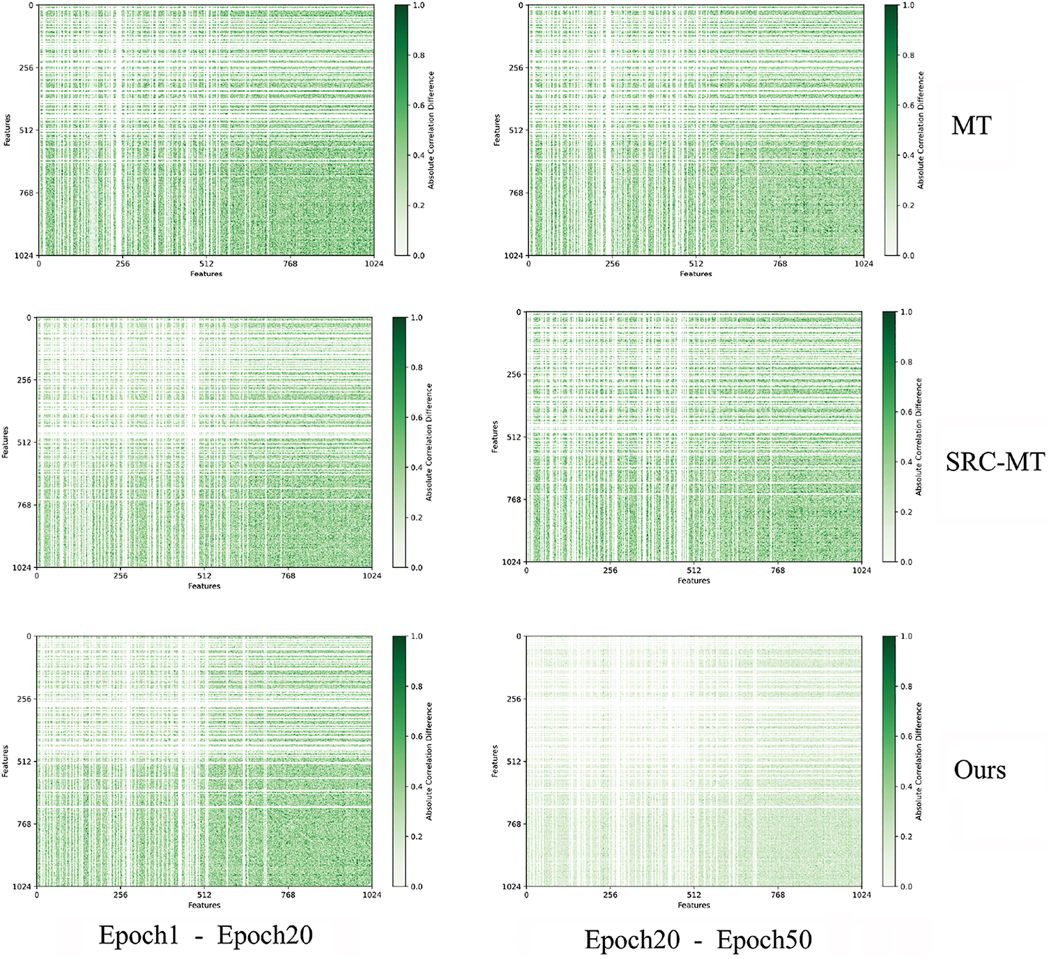
Figure 8: The absolute distance between different correlation matrices on three models

We compute the Mean Absolute Error (MAE), Mean Squared Error (MSE), and Maximum Error (MAXE) between the student feature matrix and the teacher feature matrix. Tables 5 and 6 present the results. In Table 5, we make experiments under 5%,10%, and 20% labeled data at different epochs. Observing the experimental data, we can see that our experimental results also change with training progressing and the percentages of labeled data varying. Among these, when using 20% labeled samples and at the 50th epoch, the difference between the two matrices is minimal, illustrating that the model is learning stable information to strengthen the relation between sample features under noises. Additionally, we also find that at the 1st epoch, regardless of the amount of labeled data used, the difference between the two matrices is significantly large. This may be due to the introduction of perturbations at the early training stage, which has already affected the consistency of model learning. However, at this stage, the model is not yet robust enough to capture meaningful information effectively.

We first conduct experiments on our model with 20% labeled data, and to make the conclusions more convincing, we also compute these evaluate metrics on other models, namely MT and SRC-MT. In our experiments, we calculate MAE and MAXE between the teacher feature matrix and student feature matrix at different epochs, the results are shown in Table 6. Both MAE and MAXE values decrease as training progresses, indicating that the consistency between the student and teacher feature matrices strengthens over time. This highlights that the consistency regularization model is capable of learning stable features, even in the presence of noise.

4.3 Different Loss Combinations

The ablation study of different loss combinations is shown in the following Table 7. As shown in this table, the significance of and in addressing the class imbalance problem and improving semi-supervised medical image classification is clearly demonstrated. The model is equivalent to the MT model when only using and cross-entropy loss. The second row shows the performance of the SRC-MT model, demonstrating that enforcing sample relation consistency leads to improved model performance. However, we have already analyzed that the Gram Matrix used in this model may lose some features, so we introduce CCA to explore the intrinsic relationship between samples. In the third row, we only change to , while keeping the traditional consistency loss unchanged and still using the cross-entropy loss as supervised loss. Finally, we replace the cross-entropy loss with a new loss based on the third experiment to address the issue of category imbalance, which is equivalent to our model, indicating that only when combining all unsupervised loss and supervised loss, the framework can work better.

Moreover, to compare the classification accuracy of MT, SRC-MT, and our model intuitively, we extract the logits layer features of the three models in the same period and visualize them by t-SNE method, as shown in Fig. 9. We can easily observe that each cluster becomes more clustered from MT to SRC-MT, especially NV cluster and AK cluster, but NV samples are still incorrectly predicted as MEL or BKL. In our model, the inter-class distance becomes larger, while the intra-class distance in the cluster space is smaller, and our model misjudgment probability becomes smaller, proving that our method is effective.

Figure 9: Visualization of model predictions

4.4 The Study of Loss Weighting

We investigate the effect of different on the model. The experiment is made under different loss weighting from 0 to 5, and the results are shown in the following Table 8. Obviously, the overall performance of our model is significantly improved when rises from 0 to 1. However, when increases from 1 to 5, the performance of the network is even worse, indicating that the classification ability does not increase with the increase of loss weighting, i.e., the loss weighting is not suitable for our framework to be set too large or too small. Therefore, we do all experiments with the setting as 1.

5  Discussion

We have conducted extensive experiments on the ISIC 2017 and ISIC 2018 datasets, comparing our approach with other state-of-the-art semi-supervised methods, particularly two classic consistency-based models (i.e., MT and SRC-MT). From the experimental results, our model has improved AUC, Accuracy, Sensitivity, and F1 score on the ISIC 2018 dataset, proving that focusing on feature relation indeed improves the consistency of our model and makes the most of unlabeled data.

Automated medical image classification could highly improve the productivity of medical researchers. However, obtaining high-quality labeled data is laborious and tedious work for doctors. Therefore, semi-supervised learning is a good choice for studying medical image classification. In this paper, we introduce a novel method that enforces the sample relation based on traditional consistency regular methods, exploring the semantic information of unlabeled data. Recently, we are focusing on how to address the scarcity of labeled data. In the future, we may make better use of this technology for segmentation or detection tasks. It is also an interesting work for us to explore how to utilize automatic data transformations and data generation to create better perturbation and data availability. In addition, we explore the feature relation by CCA, we could also try other methods to enforce the consistency of features.

6  Conclusions

In this paper, we present an effective method that maximizes the use of unlabeled data and addresses the issue of dataset imbalance. To prove the effectiveness of the proposed model, we conducted extensive experiments on ISIC 2017 and ISIC 2018 datasets. The results demonstrate strong performance, particularly in terms of AUC and Accuracy. In the future, we could also try to apply our CSRC model to medical segmentation.

Acknowledgement: Not applicable.

Funding Statement: This work is sponsored by the National Natural Science Foundation of China Grant No. 62271302, and the Shanghai Municipal Natural Science Foundation Grant 20ZR1423500.

Author Contributions: Funding acquisition: Kun Liu; Methodology: Chen Bao; Software: Chen Bao; Supervision: Kun Liu; Validation: Chen Bao; Writing—original draft: Kun Liu, Chen Bao; Writing—review and editing: Kun Liu, Sidong Liu. All authors reviewed the results and approved the final version of the manuscript.

Availability of Data and Materials: The dataset (i.e., ISIC2018) we used is a public dataset.

Ethics Approval: Not applicable.

Conflicts of Interest: The authors declare no conflicts of interest to report regarding the present study.

References

1. You C, Zhou Y, Zhao R, Staib L, Duncan JS. SimCVD: simple contrastive voxel-wise represen- tation distillation for semi-supervised medical image segmentation. IEEE Trans Med Imaging. 2022;41(9):2228–37. doi:10.1109/TMI.2022.3161829. [Google Scholar] [PubMed] [CrossRef]

2. Ghosh S, Bandyopadhyay A, Sahay S, Ghosh R, Santosh KC. Colorectal histology tumor detection using ensemble deep neural network. Eng Appl Artif Intell. 2021;100(3):104202. doi:10.1016/j.engappai.2021.104202. [Google Scholar] [CrossRef]

3. Yang Z, Ran L, Zhang S, Xia Y, Zhang Y. EMS-Net: ensemble of multiscale convolutional neural networks for classification of breast cancer histology images. Neurocomputing. 2019;366(Nov. 13):46–53. doi:10.1016/j.neucom.2019.07.080. [Google Scholar] [CrossRef]

4. Gipson DR, Chang AL, Lure AC, Mehta SA, Gowen T, Shumans E, et al. Reassessing acquired neonatal intestinal diseases using unsupervised machine learning. Pediatr Res. 2024;96(1):165–71. doi:10.1038/s41390-024-03074-x. [Google Scholar] [PubMed] [CrossRef]

5. Wang N, Wang H, Yang S, Dong S, Viriyasitavat W. Semi-supervised incremental domain generalization learning based on causal invariance. Int J Mach Learn Cybern. 2024;15(10):4815–28. doi:10.1007/s13042-024-02199-z. [Google Scholar] [CrossRef]

6. Naga V, Mathai TS, Paul A, Summers RM. Universal lesion detection and classification using limited data and weakly-supervised self-training. Comput Sci. 2022;13559. doi:10.1007/978-3-031-16760-7. [Google Scholar] [CrossRef]

7. Laine S, Aila T. Temporal ensembling for semi-supervised learning. In: International Conference on Learning Representations; 2016. doi:10.48550/arXiv.1610.02242. [Google Scholar] [CrossRef]

8. Dinesh Kumar MR, Paval KS, Sanghamitra S, Shrish Surya NT, Jyothish Lal G, Ravi V. Mean teacher model with consistency regularization for semi-supervised detection of COVID-19 using cough recordings. Vol. 865. In: Fourth congress on intelligent systems; 2024. p. 95–108. [Google Scholar]

9. Yao P, Shen S, Xu M, Liu P, Zhang F, Xing J, et al. Single model deep learning on imbalanced small datasets for skin lesion classification. IEEE Trans Med Imaging. 2022;41(5):1242–54. doi:10.1109/TMI.2021.3136682. [Google Scholar] [PubMed] [CrossRef]

10. Rahmouni A, Sabri MA, Ennaji A, Aarab A. Skin lesion classification based on vision transformer (ViT). Vol. 837. In: Artificial intelligence, data science and applications. Cham: Springer; 2024. p. 472–7. doi:10.1007/978-3-031-48465-0_63. [Google Scholar] [CrossRef]

11. Yu L, Chen H, Dou Q, Qin J, Heng P-A. Automated melanoma recognition in dermoscopy images via very deep residual networks. IEEE Trans Med Imaging. 2017;36(4):994–1004. doi:10.1109/TMI.2016.2642839. [Google Scholar] [PubMed] [CrossRef]

12. Shen XB, Sun QS, Yuan YH. Orthogonal canonical correlation analysis and its application in feature fusion. In: Proceedings of the 16th International Conference on Information Fusion; 2013. p. 151–7. [Google Scholar]

13. Codella NCF, Gutman D, Celebi ME, Helba B, Marchetti MA, Dusza SW, et al. Skin lesion analysis toward melanoma detection: a challenge at the 2017 international symposium on biomedical imaging (ISBIhosted by the international skin imaging collaboration (ISIC). In: 2018 IEEE 15th International Symposium on Biomedical Imaging (ISBI 2018); 2018. p. 168–72. [Google Scholar]

14. Tschandl P, Rosendahl C, Kittler H. The HAM10000 dataset, a large collection of multi-source dermatoscopic images of common pigmented skin lesions. Sci Data. 2018;5(1):1–9. doi:10.1038/sdata.2018.161. [Google Scholar] [PubMed] [CrossRef]

15. Xie Y, Zhang J, Xia Y. Semi-supervised adversarial model for benign-malignant lung nodule classification on chest CT. Med Image Anal. 2019;57(2):237–48. doi:10.1016/j.media.2019.07.004. [Google Scholar] [PubMed] [CrossRef]

16. Liu L, Tan RT. Certainty driven consistency loss on multi-teacher networks for semi-supervised learning. Pattern Recognit. 2021;120(3):108140. doi:10.1016/j.patcog.2021.108140. [Google Scholar] [CrossRef]

17. Zhou Z, Tarzanagh DA, Hou B, Tong B, Xu J, Feng Y, et al. Fair canonical correlation analysis. Red Hook, NY, USA: Curran Associates Inc; 2024. [Google Scholar]

18. Andrew G, Arora R, Bilmes J, Livescu K. Deep canonical correlation analysis. In: Proceedings of the 30th International Conference on Machine Learning; 2013; Vol. 28, pp. 1247–55. [Google Scholar]

19. Zhang X, Hao Y, Zhang J, Zou S, Xie S, Du L. Improved multi-task scca for brain imaging genetics via joint consideration of the diagnosis, parameter decomposition and network constraints. In: 2021 IEEE International Conference on Bioinformatics and Biomedicine (BIBM); 2021. p. 1159–64. [Google Scholar]

20. Zhang J, Shang M, Xie Q, Zhang M, Xi D, Guo L, et al. A sparse multi-task contrastive and discriminative learning method with feature selection for brain imaging genetics. In: 2022 IEEE International Conference on Bioinformatics and Biomedicine (BIBM); 2022. p. 660–5. [Google Scholar]

21. de Boer PT, Kroese DP, Mannor S, Rubinstein RY. A tutorial on the cross-entropy method. Ann Oper Res. 2005;134(1):19–67. doi:10.1007/s10479-005-5724-z. [Google Scholar] [CrossRef]

22. Gessert N, Sentker T, Madesta F, Schmitz R, Kniep H, Baltruschat I, et al. Skin lesion diagnosis using ensembles, unscaled multi-crop evaluation and loss weighting. arXiv:1808.01694. 2018. [Google Scholar]

23. Cui Y, Jia M, Lin TY, Song Y, Belongie S. Class-balanced loss based on effective number of samples. In: 2019 IEEE/CVF Conference on Computer Vision and Pattern Recognition (CVPR); 2019. p. 9260–9. [Google Scholar]

24. Battaglia PW, Hamrick JB, Bapst V, Sanchez-Gonzalez A, Zambaldi V, Malinowski M, et al. Relational inductive biases, deep learning, and graph networks. arXiv:1806.01261. 2018. [Google Scholar]

25. Liu Q, Yu L, Luo L, Dou Q, Heng PA. Semi-supervised medical image classification with relation- driven self-ensembling model. IEEE Trans Med Imaging. 2020;39(11):3429–40. doi:10.1109/TMI.2020.2995518. [Google Scholar] [PubMed] [CrossRef]

26. Gatys LA, Ecker AS, Bethge M. A neural algorithm of artistic style. J Vis. 2015. doi:10.48550/arXiv.1508.06576. [Google Scholar] [CrossRef]

27. Sergievskiy N, Ponamarev A. Reduced focal loss: 1st place solution to xView object detection in satellite imagery. arXiv:1508.06576. 2019. [Google Scholar]

28. Faber K, Zurek D, Pietron M, Japkowicz N, Vergari A, Corizzo R. From MNIST to imagenet and back: benchmarking continual curriculum learning. Mach Learn. 2024;113(10):8137–64. doi:10.1007/s10994-024-06524-z. [Google Scholar] [CrossRef]

29. Kingma DP, Ba J. Adam: a method for stochastic optimization. In: 3rd International Conference for Learning Representations; 2015. doi:10.48550/arXiv.1412.6980. [Google Scholar] [CrossRef]

30. Lima DM, Rodrigues JFJr., Brandoli B, Goeuriot L, Amer-Yahia S. DermaDL: advanced convolutional neural networks for computer-aided skin-lesion classification. SN Comput Sci. 2021;2(4):253. doi:10.1007/s42979-021-00641-5. [Google Scholar] [CrossRef]

31. Xu Z, Iwaihara M. Self-training involving semantic-space finetuning for semi-supervised multi-label document classification. Int J Digit Libr. 2024;25(1):25–39. doi:10.1007/s00799-023-00355-4. [Google Scholar] [CrossRef]

32. Wei C, Liang J, Liu H, Hou Z, Huan Z. Multi-stage unsupervised fabric defect detection based on dcgan. Vis Comput. 2023;39(12):6655–71. doi:10.1007/s00371-022-02754-1. [Google Scholar] [CrossRef]