A Barrier-Based Machine Learning Approach for Intrusion Detection in Wireless Sensor Networks

1  Introduction

Industries such as healthcare, agriculture, military, and environmental monitoring widely deploy Wireless Sensor Networks (WSNs) to enable real-time data collection in remote and critical locations. Despite their versatility, WSNs face unique security challenges due to resource constraints in processing power, energy, and memory [1,2]. These limitations make traditional intrusion detection techniques inadequate, leaving WSNs vulnerable to attacks like data tampering, eavesdropping, and unauthorized access. To address these issues, a barrier-based machine learning approach offers a promising solution by enhancing detection accuracy and efficiency and balancing security needs with the network’s resource limitations.

Due to their inherent limitations, such as low computational power, Wireless Sensor Networks (WSNs) face unique security challenges that restrict the complexity of implemented security algorithms. Limited bandwidth poses difficulties in securely transmitting large amounts of data, making it challenging to deploy robust encryption methods. Additionally, resource constraints, such as battery life and memory, hinder the ability to perform extensive security checks or maintain constant monitoring, making WSNs vulnerable to attacks like data tampering and unauthorized access.

Protecting WSNs is important, especially in applications that deal with sensitive information and infrastructure [3]. Therefore, Intrusion Detection System (IDS monitors network or system activities for unauthorized access and anomalies, detecting threats and generating alerts to enhance security) has become vital in securing WSNs by identifying malicious activities and preventing attacks. IDS techniques encounter challenges in adapting to new offensive approaches due to the limited resources of WSNs, which differ from those of ordinary systems. Overcoming these challenges may involve implementing machine learning techniques that rely on past data so that they can change accordingly, leading to better performance. Artificial neural networks (ANNs) have extensively researched intrusion detection, providing a good representation of data relationships.

They can detect the most advanced attacks on WSNs by effectively analyzing data sets in their arrangements [4]. Nonetheless, artificial neural networks may face challenges regarding relations among data. The Convolutional Neural Networks (CNNs) and Long Short-Term Memory (LSTM), which combines convolutional networks and LSTM, is one way to overcome this limitation. Combining the temporal sequential learning abilities of LSTMs with the feature extraction abilities of CNNs, these models can keep an eye on intrusive patterns that constantly change [5]. Intrusion detection involves identifying access and seeking the completeness and trustworthiness of collected information. Traditional security techniques may be insufficient since wireless sensor networks operate in harsh environments. Machine-learning-based models solve this problem by adapting to trends and improving performance over time. For instance, artificial neural networks are good at processing huge data volumes and recognizing difficult infiltration scenarios. Hybrid models such as CNN LSTM effectively detect attacks supported by sources that exhibit temporal patterns [5,6].

Virtual barriers are logical partitions within a network that create multiple decision boundaries to separate different classes of network traffic, particularly in the context of intrusion detection [7]. By segmenting the network through these barriers, the system can monitor and analyze traffic more effectively, allowing for targeted detection of anomalies (Fig. 1). By adequately representing both normal and malicious activities in the monitoring process, this approach addresses the issue of imbalanced data. It enhances the accuracy and robustness of intrusion detection models.

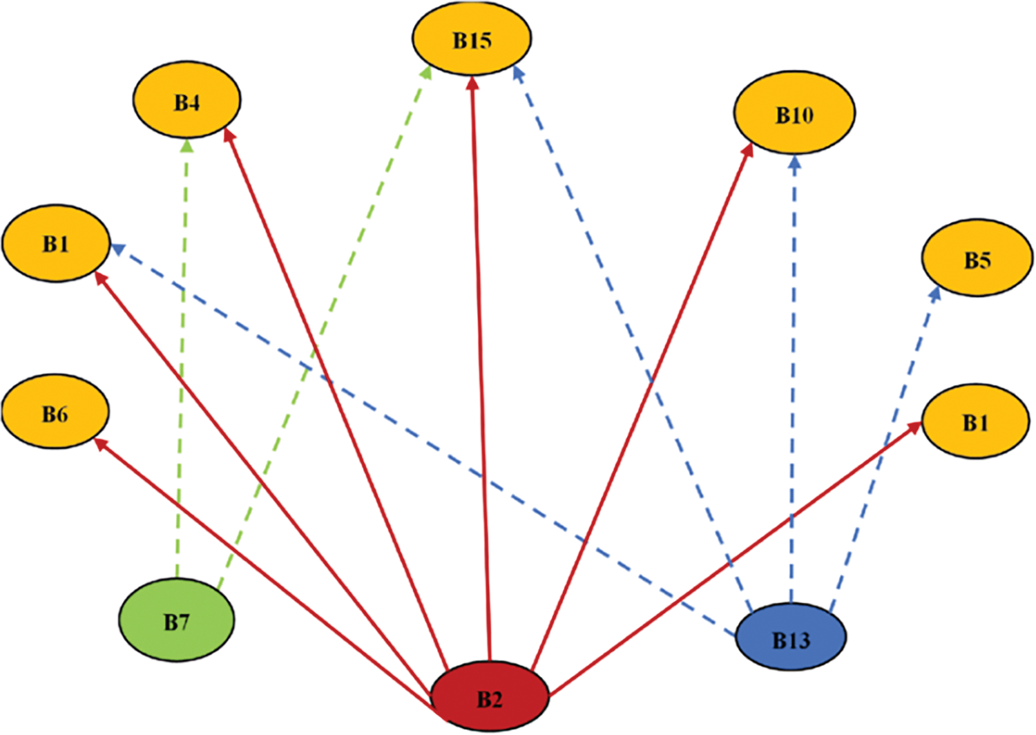
Figure 1: Influence map of barriers

This research selects logistic regression (LR) as the model due to its simplicity and interpretability, serving as a benchmark for more complex models. Despite its simplicity, LR proves to be an effective IDS [8]. Conversely, the XGBoost algorithm is familiar with ensemble learning and specializes in highly effective techniques for handling imbalanced data sets, including regularization. This makes it highly useful in intrusion detection for wireless sensor networks (WSN) [9]. Successful ensemble models have been exploiting multiple predictions from many learners, enhancing generalization while avoiding overfitting in different machine learning domains like IDS [10]. In this way, using a model such as regression, we create a strong baseline and benchmark to evaluate against more complex models that are harder to interpret [11]. Simultaneously, the XGBoost algorithm enhances its applicability in IDSs within sensor networks by managing imbalanced datasets and implementing regularisation methods, thereby achieving a trade-off between accuracy and computational efficiency [12].

We have improved these models by using a group of base learners like Random Forest, Gradient Boosting, and XGBoost, which overcome generalisation and minimise overfitting. This makes them more suitable for intrusion detection, as they effectively handle variations and noise in the data from sensor networks [13]. This study tests the performance of these models using Monte Carlo simulations based on sensor distributions, even when modelling an actual WSN [14]. The other methods involve Random Forest (RF), Gradient Boosting (GB), and XGBoost as comparative benchmarks for their robustness against random fluctuations and interference within WSN networks.

The problem domain revolves around intrusion detection in wireless sensor networks (WSNs), which are increasingly utilized in critical applications such as healthcare, environmental monitoring, and smart cities. These networks consist of numerous sensor nodes that collect and transmit data wirelessly, making them vulnerable to various security threats, including unauthorized access and denial-of-service attacks. The challenge is exacerbated by the imbalanced nature of network traffic, where normal activities vastly outnumber malicious events, leading to difficulties in accurately detecting intrusions. This necessitates the development of effective machine learning models that can adapt to the dynamic and resource-constrained environment of WSNs while ensuring timely and reliable detection of anomalies.

The rest of this paper is structured as follows: Section 2 presents the literature review, providing an overview of previous research in the field. Section 3 describes the network-on-chip architecture, detailing its components and functionality. On the other hand, Sections 4 & 5 discuss the proposed methodology, including the barrier-based machine learning approach and the implementation of the CNN-LSTM model. Sections 6 & 7 present the experimental results and performance evaluation of the proposed method, while Section 8 concludes the paper with a summary of findings and suggestions for future research.

A. The Problem Statement

Wireless Sensor Networks (WSNs) face significant security challenges, particularly due to their inherent limitations such as low computational power and the prevalence of imbalanced data in network traffic. Traditional Intrusion Detection Systems (IDS) often struggle to accurately identify and mitigate threats in WSNs, primarily because they are designed to handle datasets where normal traffic significantly outweighs malicious instances. This imbalance can lead to high false negative rates, where intrusions go undetected.

Moreover, existing methodologies for addressing data imbalance, such as partitioning networks into logical sections, have been explored but often lack integration with advanced machine learning techniques that can effectively capture complex patterns in network traffic. As a result, there is a pressing need for a more effective approach that addresses the issue of imbalanced data and enhances the accuracy and robustness of intrusion detection in WSNs.

The study aims to develop a novel barrier-based machine-learning technique that partitions the network into virtual barriers, allowing for focused monitoring and data collection tailored to specific traffic patterns. This approach seeks to improve the diversity of the training dataset and leverage advanced models like CNN-LSTM to enhance detection accuracy, ultimately contributing to more reliable security solutions for WSNs.

B. The Contributions

The paper aims to present a barrier-based machine learning technique that offers a more accurate approach to dealing with data imbalance in intrusion detection for wireless sensor networks (WSNs) by dividing the network into logical partitions or virtual barriers. This allows for focused monitoring and data collection tailored to specific traffic patterns, enhancing the diversity of the training dataset. Additionally, it integrates advanced machine learning models, such as CNN-LSTM, that effectively capture temporal patterns in network traffic, improving detection accuracy and robustness against complex attack patterns. This combination addresses scalability and computational limitations more effectively than previous approaches. This research has the following major contributions:

•   Novel Barrier-Based Technique: Introducing a method using virtual barriers to address imbalanced data in intrusion detection.

•   Hybrid Model Implementation: Development of a CNN-LSTM model that captures spatial and temporal patterns in network traffic.

•   Comparative Model Evaluation: Assessment of multiple machine learning models, including ANN, linear regression, and ensemble models.

•   Focus on Imbalanced Data: Addressing challenges of imbalanced datasets to improve detection accuracy.

•   Monte Carlo Simulations: Simulations are used to derive key features for model training.

•   Performance Metrics: Establish R-squared and RMSE to evaluate model performance in intrusion detection.

2  Literature Review

Network Intrusion Detection Systems (NIDS) are essential for identifying and flagging suspicious activities within Wireless Sensor Networks (WSNs) and the Internet of Things (IoT). Recent advancements have introduced various methodologies to improve detection accuracy and efficiency.

The researchers in [15] employed a feature selection method, FA-ML, in conjunction with the Support Vector Machine (SVM) model for classification. They also utilized the GWO algorithm to adjust parameters for detecting intrusions in WSN-IoT environments. Another study in [16] combined LSTM networks for classification with Extreme Gradient Boosting (XGBoost) and CNN for feature extraction, significantly enhancing detection accuracy in wireless networks.

Moreover, researchers proposed a multi-tiered intrusion detection system (MDIT) [17], integrating hybrid deep learning models. This system leverages the strengths of CNNs for data collection and LSTMs for capturing temporal information in network messages. A different study in [18] introduced a methodology for analyzing information that successfully identified four distinct types of DoS attacks when paired with classification techniques.

Research in [19] presented the VG-IDS model to improve recommendation systems, which incorporates context awareness by considering user preferences alongside system attributes. Additionally, the NSL-KDD dataset was utilized in a study in [20] that implemented a Recurrent Neural Network with Long Short-Term Memory (RNN-LSTM) approach for classifying intrusions in WSNs.

An AutoML model was proposed in a study in [21], employing Bayesian optimization to fine-tune hyperparameters and automatically select suitable machine learning models, including Support Vector Regressors (SVR) and Boosted Decision Trees (BDT). This model aims to accurately predict barriers to rapid intrusion detection and prevention systems, utilizing Monte Carlo simulations to derive key predictors such as region area and sensor transmission range.

One notable study in [22] developed a computer-based WSN detection system that utilized a Convolutional Neural Network-Long Short-Term Memory (CNN-LSTM) model. This research employed the NS-2 network simulator to create a simulated wireless environment, using the Low Energy Adaptive Clustering Hierarchical (LEACH is a routing protocol for wireless sensor networks that forms clusters to optimize energy use and extend network lifespan) routing protocol to gather data. The researchers preprocessed the collected data to generate 23 features that characterize the condition of each sensor while also implementing five different types of Denial of Service (DoS) attacks during the simulationrouting protocol to gather data. The researchers preprocessed the collected data to generate 23 features that characterize the condition of each sensor while also implementing five different types of Denial of Service (DoS) attacks during the simulation.

In another approach, the authors of [23] presented an upgraded CNN model incorporating improved parameters obtained through the Grey Wolf Optimiser (GWO) technique. This optimization process enhanced the CNN’s predictive accuracy. Additionally, the model utilized transfer learning, allowing knowledge gained from the CNN-LSTM model to be applied in subsequent iterations, thereby improving detection accuracy. The effectiveness of this model was evaluated using two online industrial IDS datasets, ToN-IoT and UNW-NB15, for multi-class classification analysis.

In recent studies, various models have been evaluated for their performance in intrusion detection systems, with notable metrics highlighted in Table 1. These findings illustrate the advancements made in machine learning techniques for enhancing accuracy and addressing challenges such as data imbalance in wireless sensor networks.

3  Network on Chip Architecture (NoC)

The selection of models used in this study for forecasting barriers in Wireless Sensor Networks (WSNs) is based on their unique strengths and suitability for the task at hand.

These models were chosen for their complementary strengths in handling the unique challenges of forecasting barriers in WSNs, including the need for accuracy, adaptability to evolving attack patterns, and the ability to manage imbalanced data effectively. Each model contributes to a comprehensive approach to intrusion detection, enhancing the overall robustness and reliability of the system.

3.1 Feedforward ANN

A Neural Network (NN) is a computational model that simulates the brain’s simplified functioning to accomplish a specific job. The main goal of the neural network (NN) model is to determine a mapping function (f) that can accurately predict a target function (f*) by training the NN using labelled training datasets. During the training phase, the network acquires an understanding of the different parameters in the training data. After the model has undergone training, it is crucial to test and evaluate its performance with data that has not been previously observed.

This formula arises from the need to compute the weighted sum of inputs, which is then transformed by an activation function to introduce non-linearity, allowing the network to learn complex patterns in the data.

(1)

where:

: Weight connecting neuron i in layer l − 1 to neuron j in layer l,

: Activation of neuron i in the previous layer,

: Bias of neuron j in layer l,

: Linear combination of inputs to neuron j in layer l.

(2)

where f is the activation function (e.g., sigmoid, ReLU, tanh).

3.2 Hybrid Models CNN-LSTM

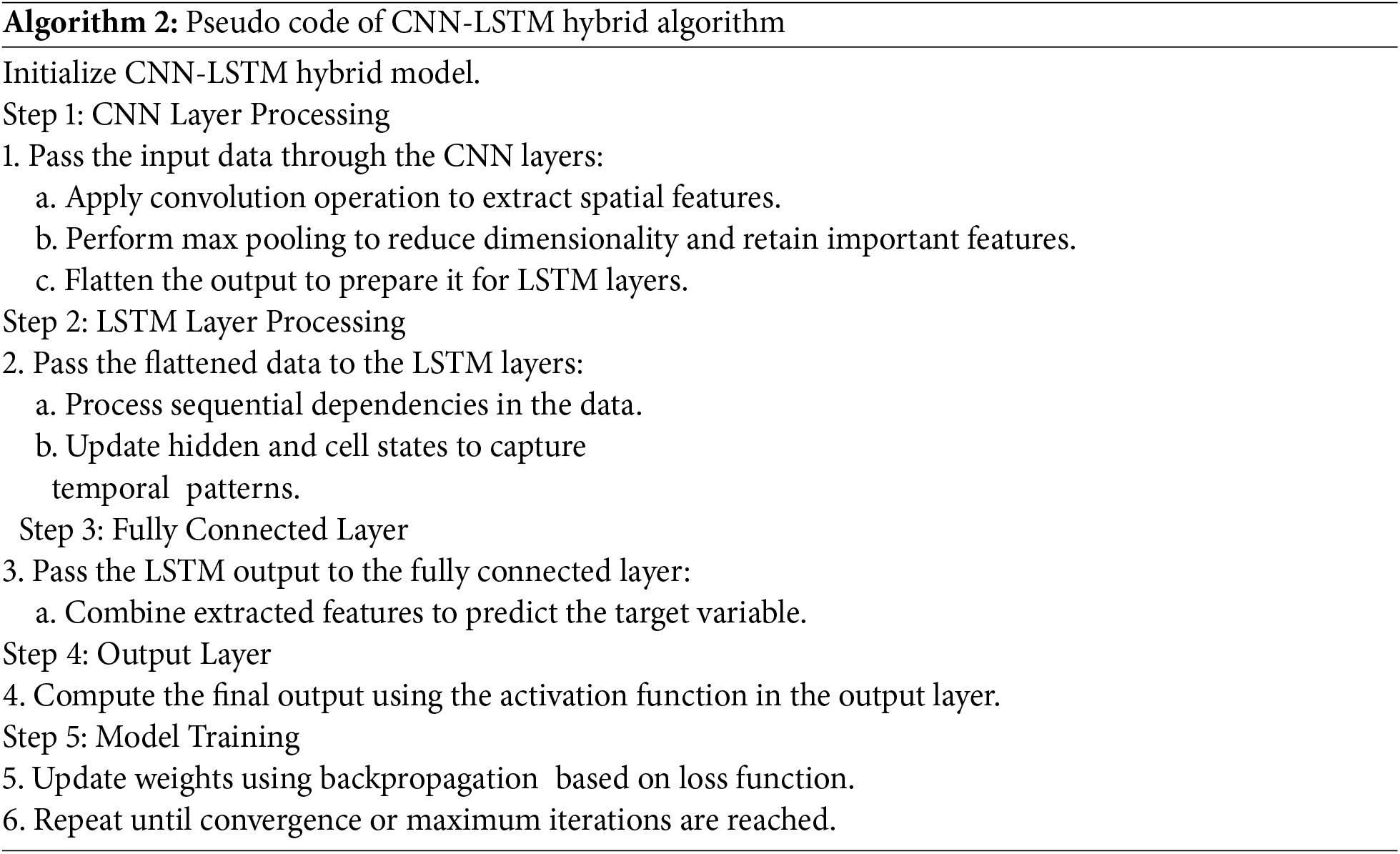
Each of the CNN and LSTM models has unique characteristics. To forecast the barriers in WSN, a hybrid CNN-LSTM model that combines the best features of both LSTM and CNN models was created for this work. Initially, CNN layers comprised the top layer of the CNN–LSTM architecture. CNN consists of many hidden layers: an output layer that extracts features for LSTM cells and an input layer that enters the input variables. An activation function, a pooling layer, and a convolution layer are often components of the hidden layer. The fully linked layer receives its input from the LSTM’s output. Conventional neural networks cannot learn sequential aspects of inputs; the CNN layers handle long-range dependencies to handle these features, which are then included by the bottom LSTM layer for target value prediction.

3.3 Logistic Regression

It is a method of data analysis that draws connections between two parameters from isolated data by applying mathematics. It distinguishes one generic individual from the rest using these ratios. A forecast can only have a finite set of possible outcomes (final values), like yes or no.

This formula arises from the need to model the relationship between the independent variables and the log-odds of the dependent variable, allowing for effective classification of intrusion events.

(3)

where:

X: input feature vector,

W: weight vector,

b: bias term.

3.4 XGB Regressor

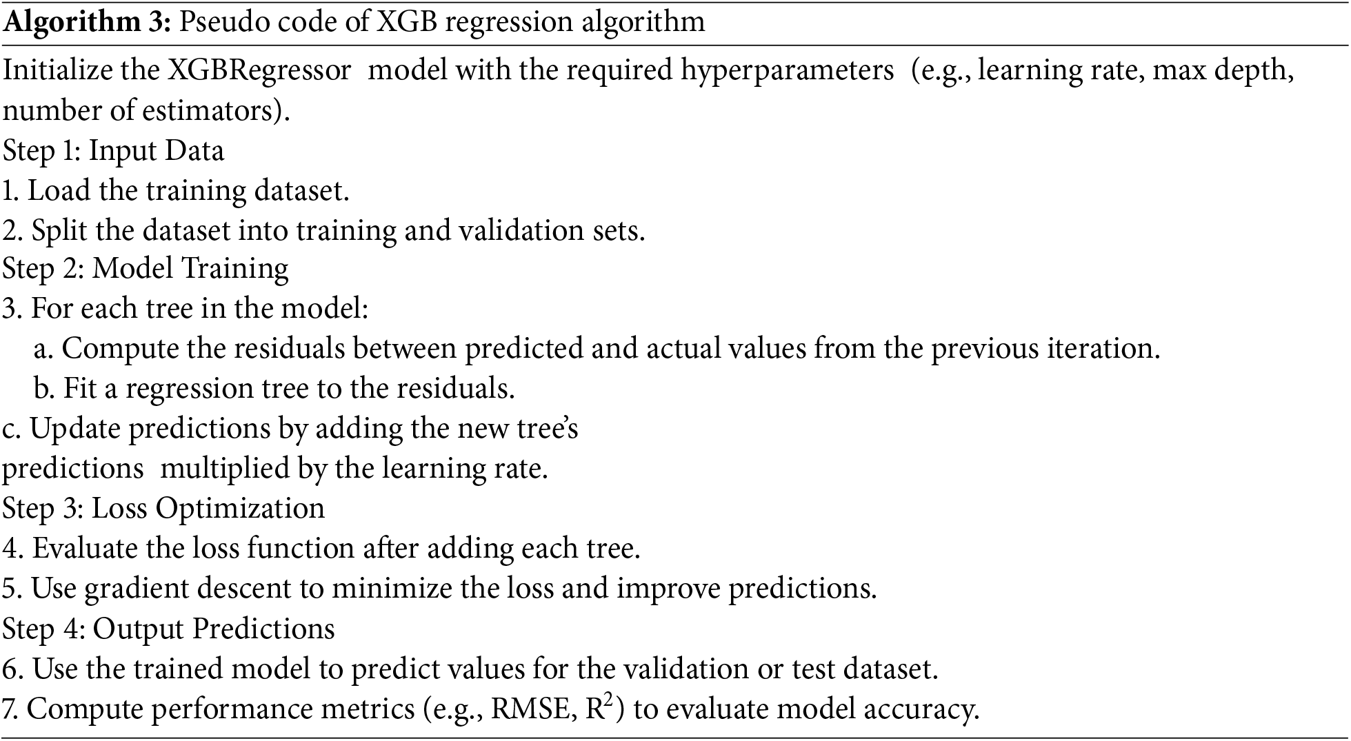
It is a strong method for creating models of supervised learning. Knowing about the (XGBoost) objective function and base learners helps deduce this proposition’s veracity. Loss function and a regularisation term abound in the objective function. It explains how far the model outputs are from the true values—the difference between actual and expected values. For XGBoost’s regression issues, reg: linear is the loss function that most often occurs; for binary classification, reg: logistics. XGBoost is one of the ensemble learning techniques; ensemble learning is training and integrating individual models (called base learners) to produce a single prediction. XGBoost wants the base learners.

The formulation arises from minimising the loss while controlling for model complexity, making XGBoost effective for handling various data types, including imbalanced datasets.

(4)

where are decision trees in the model and is the space of all possible trees.

3.5 Ensemble Model

It involves the execution of two or more related but distinct analytical models, followed by the synthesis of the results into a singular score or spread. Applications for data extraction and predictive analytics benefit from this. In this study, the ensemble model contained a combination of Random Forest (RF), Gradient Boosting, and XGBoost, which were used to improve detection as part of the ensemble method (Fig. 2).

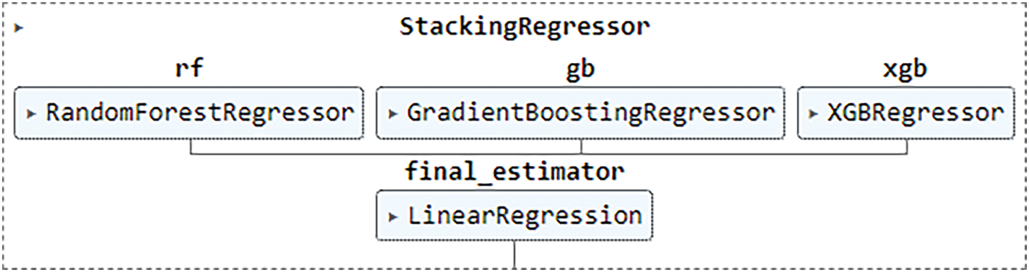
Figure 2: The ensemble model contains (RF, GB, and XGB models)

The formula arises from the principle that combining multiple models can lead to better generalization and robustness, particularly in the context of complex and evolving intrusion detection scenarios

(5)

where are models, and are their weights.

3.6 Baseline Model

3.6.1 Random Forset (RF)

(6)

where is the prediction from the i-th tree, and N is the total number of trees.

This versatile tool can be applied to both regression and classification tasks. It relies on a decision tree. Random samples are obtained from datasets, and a tree is created for each sample. Each decision tree generates a prediction; then a voting process is conducted [34,35]. The decision tree with the most votes is utilised to make predictions. The random forest technique exhibits great accuracy but is characterised by its complexity and demands substantial processing time and resources.

3.6.2 Gradient Boosting

It is an approach [36] that constructs a predictor model for regression and classification tasks by utilising weak predictive models like decision trees. We can halt the process at this point if there isn’t a pattern that can be modelled because an overfitting issue could arise.

(7)

where I is the loss function, are true values, and are predictions.

4  Dataset

Preprocessing the data before feeding it into the models is crucial to ensure effective learning and accurate predictions. The data is normalized to scale the features to a common range, which helps improve model convergence during training. This step ensures that features with larger ranges do not disproportionately impact model performance. Missing data is also handled using a common imputation technique (mean values) and missing records are removed to maintain the integrity of the dataset. Generally, a well-defined preprocessing pipeline, including normalization and handling of missing data, is essential to prepare the dataset for machine learning models, ensuring that the data is clean and suitable for analysis in the context of wireless sensor networks (WSNs).

The barrier-based approach addresses data imbalance by partitioning the network into logical sections, or virtual barriers, which allows for more focused monitoring and data collection. Each barrier can be tailored to capture traffic patterns specific to its segment, ensuring that normal and malicious activities are represented more evenly. This targeted monitoring helps mitigate the skewed distribution often seen in network traffic, where normal traffic significantly outweighs malicious instances.

Balancing data collection across these partitions enhances the training dataset’s diversity, leading to improved model performance. It allows machine learning models to learn from a more representative sample of both classes, reducing bias towards the majority class. Consequently, this results in higher detection rates for minority class instances, ultimately improving the overall accuracy and robustness of the intrusion detection system.

The dataset features six columns [25]. The first four columns match the input characteristics—area, sensing range, transmission range, and sensor count. The last two columns represent the target or response variable—especially the counts of barriers (Gaussian) and those with a standardized count. This data allows us to create machine learning models to precisely estimate the obstacles required for rapid IDS and prevention. The finished dataset has been randomly split into three parts: 70% for training, 20% for validation, and 10% for testing of all algorithms. This division was achieved using the Mersenne Twister generator (MTG).

4.1 Monte Carlo Simulations

To foretell the results of an unpredictable occurrence, mathematicians use the Monte Carlo simulation. This method enables computer programmers to analyses historical data and predict future results based on user input.

4.1.1 Sensor Distribution Scenarios

It refers to the spatial patterns of sensor deployment, typically Gaussian or uniform, impacting data generation and model performance in WSNs.

Gaussian Distribution: As demonstrated by the normal distribution, data points closer to the mean occur more frequently than those farthest from the mean, a symmetrical probability distribution around the mean.

Uniform Distribution: All possible events have an equal chance of happening, called a symmetric probability distribution. It is called a uniform distribution because each number in the range has the same chance of happening.

4.1.2 Simulation Features

•   Circular Area Size

It refers to the radius of the monitored region within which sensors are deployed in a WSN.

(8)

where:

π = Pi

r = Radius of the circle.

•   Sensing Range

It indicates the farthest distance a system of sensors or a sensor itself can precisely detect, measure, or compile data regarding a given variable or group of variables.

(9)

where:

A = The total area of the deployment region

N = The number of sensor nodes deployed in the region.

•   Communication Range

It refers to the maximum distance a sensor can transmit data to other sensors or a central node in a WSN.

(10)

where:

P = The transmission power of the sensor node

G_t = The transmitter antenna gain

G_r = The receiver antenna gain

λ = The wavelength of the transmitted signal

P_r = The minimum required receiver power.

•   Number of Sensors

It indicates the total count of individual sensors deployed within a wireless sensor network to monitor and collect data from the environment, as explained in Table 2 and Fig. 3.

(11)

where:

A = The total area of the deployment region

r = The sensing range of each sensor node.

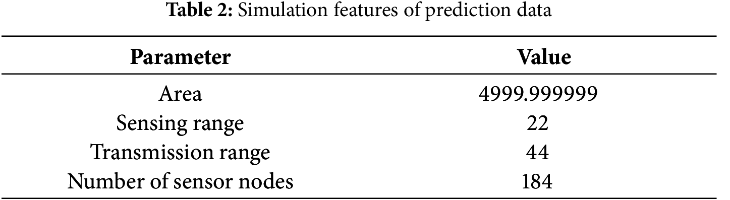
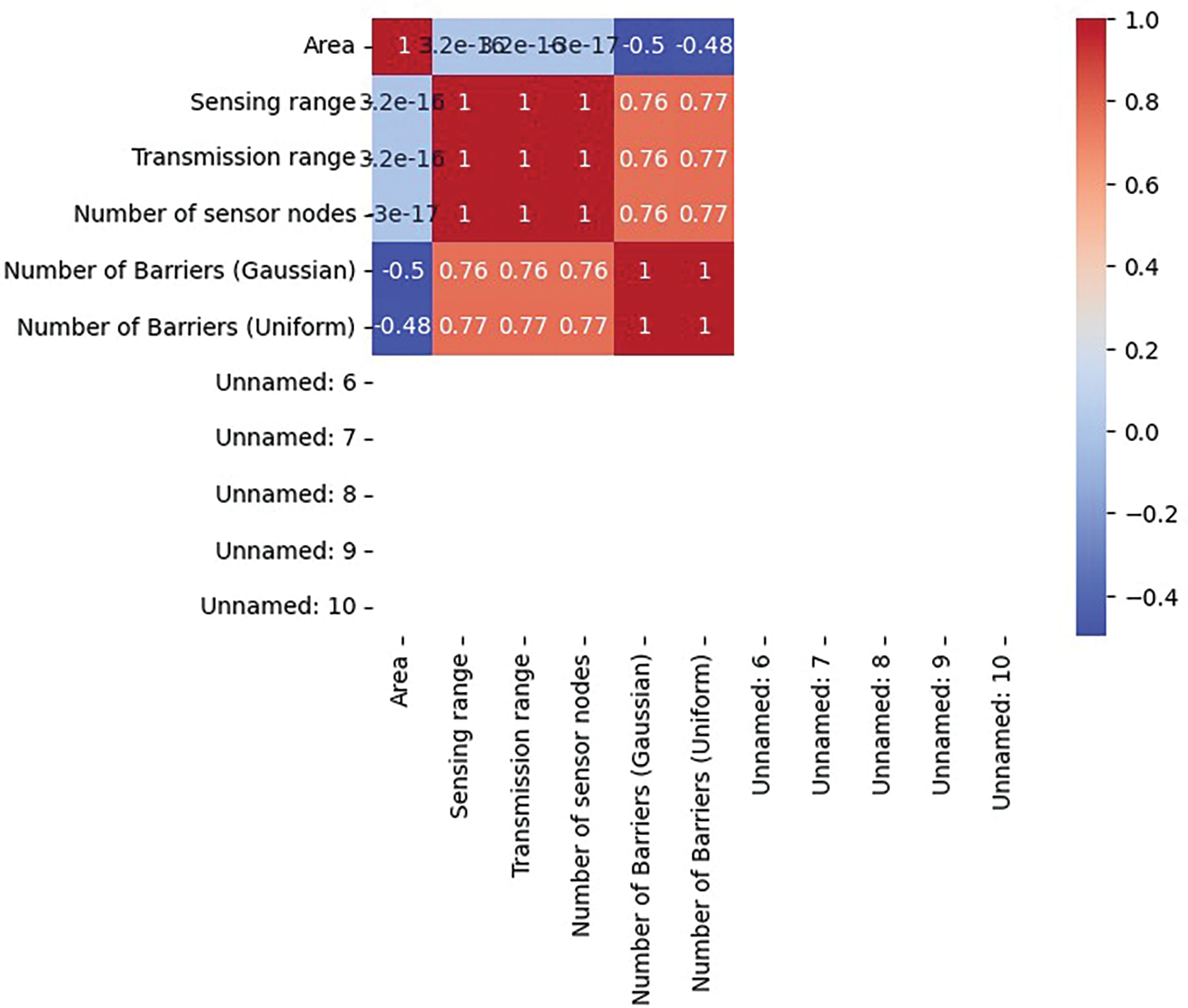
Figure 3: Exploratory data analysis

5  System Setup

5.1 Feature Extraction

Four essential factors for training the IDS models were determined: The parameters to consider are the dimensions of the circular region, the scope of detection and communication distance of the sensors, and the overall number of sensors. These aspects were selected based on their pertinence to the operation and safeguarding of WSNs. The dimensions of the circular region impact the extent of network coverage. At the same time, the sensing range determines the ability to identify objects. The communication range directly affects the efficiency of data transmission, and the number of sensors defines the density and resilience of the network.

5.2 Implementation

Step 1: Distributions for Traffic Evaluation

Gaussian and uniform distributions were utilized to evaluate machine learning models in Wireless Sensor Networks (WSNs) under varying traffic patterns.

Step 2: Gaussian and Uniform Traffic Patterns

•   Gaussian Distribution: Represents predictable, normal traffic patterns, allowing models to effectively learn and identify anomalies that deviate from expected behaviour, enhancing intrusion detection accuracy.

•   Uniform Distribution: Reflects erratic or unpredictable traffic, ensuring models can adapt to varied conditions and detect intrusions even when traffic does not follow typical patterns.

By incorporating both distributions, the study ensures a comprehensive assessment of model performance, leading to a robust and adaptable intrusion detection system capable of handling the dynamic nature of network traffic.

Step 3: Preprocessing and Feature Analysis

Predicting and regression problems are solved using machine learning techniques. The kernel approach converts the inputs into a supervised machine-learning technique, finding a single optimal bound for the possible outputs. The sensor operates to convert the inputs into a high-dimensional feature space representation. The models classify the data using the outputs of the ideal hyperplane, which are produced by labeling data partitioning. Preprocessing is required before classifier application on unstructured data. We classed the dataset using MTG. Feature analysis used several other normalized dataset characteristics to disperse the values between (+1−1). Once every aspect’s significance was assessed, weights were assigned to the pertinent features. These weights were included to increase the sensor function capacity. Then, using these weights, the relevance of every chosen trait was assessed against one another. We reweighted each variable in the training set using a sigmoid kernel function since the dataset we worked with lacked the structure to manage all the classifiers. Two fundamental ideas define weight estimation: first, the absence of a feature leads to the seeming absence of any extended structures with that feature; second, the frequency with which the feature is present is exactly connected to the importance of that feature.

Step 4: Training and Testing Workflow

The output data serves training or testing purposes depending on whether the system is in the testing or training phases. The training error concerning output data will be computed if the system is still training. So, this provides a broad notion of the algorithm’s capacity to deduce the functional impact from the data. Should the model be trained on the input data, the intended responses could be discovered in the model’s output.

The connected feedforward ANN is created by arranging neurons to connect neurons of each layer to their neighboring forward layers. From the input neurons to.

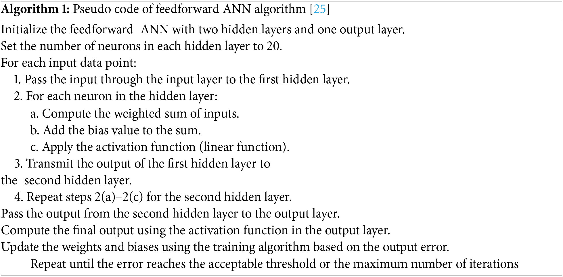
The output sensors primarily transmit the data forward, passing through hidden sensors. The total activation function of a layer is equal to the total output value because each neuron has a single activation function. The training algorithm normalizes the value of the sensor connection weight using the output results [37,38]. A single hidden layer and a feedforward ANN can approximate any continuous function. However, learning may be impossible if the required hidden size is large. Non-sequential or time-independent data are suitable for feedforward ANN. Our feedforward ANN has two hidden layers and one output layer. Each hidden layer has twenty neurons. Each neuron in the hidden layers receives a common bias value that is added to it and then activates a linear function.

Step 5: Algorithm Implementation

Hybrid models (CNN-LSTM, XGBRegression, Linear Regression, StackingRegressor) were trained on the WSN dataset, utilizing corresponding pseudo-code implementations for performance evaluation (Algorithm 1).

For the hybrid models CNN-LSTM, the following code has been trained to the WSN dataset (Algorithm 2).

For the XGBRegression, the following code has been trained to the WSN dataset (Algorithm 3).

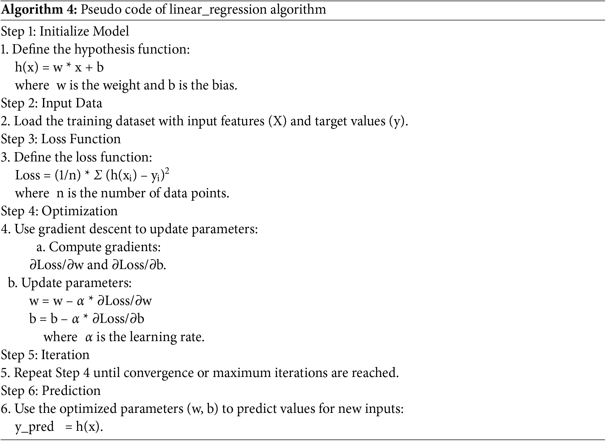
For the linear regression model, the following code has been trained to the WSN dataset (Algorithm 4).

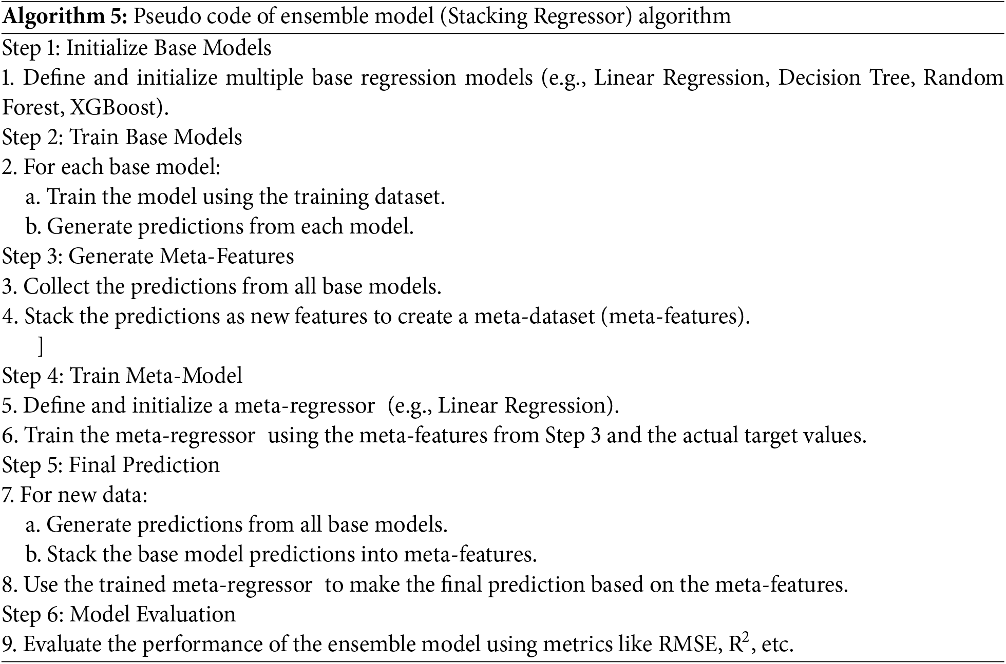
For the ensemble model (Stacking Regressor), the following code has been trained to the WSN dataset (Algorithm 5).

5.3 Hyper-Parameters for ML Models

This study selected the hyperparameters using a grid search and Bayesian optimization techniques. Grid search was employed to systematically explore a broad range of possible values for each hyperparameter (Table 3). At the same time, Bayesian optimization was used to fine-tune the selections by modeling the performance of the machine learning models as a function of the hyper parameters [39,40]. This approach allowed for the efficient identification of the optimal hyper-parameters that balance model accuracy, computational cost, and robustness in intrusion detection within Wireless Sensor Networks (WSNs). The selected hyperparameters appear to be a well-balanced set of choices based on established best practices in machine learning for wireless sensor network applications [39–41].

All models’ overfitting risks were managed through dropout layers and early stopping based on validation performance. These strategies helped improve the model’s generalization to unseen data.

5.4 Performance Metrics

There are different ways to judge the success of a model based on the type of function and how it will be used. For example, R2 and RMSE numbers are often used to judge how well regression-based models work when we want to make predictions or estimates. Each performance measure can find a statistical study of its accuracy and how much the indicators and variables of interest vary. Performance metrics employed were R and RMSE. A high value of R indicates a strong agreement between the projected values and the observed value. A smaller RMSE number indicates a higher level of accuracy in the model.

A positive bias indicates an overestimation, while a negative bias indicates an underestimation. Subsequently, we conducted error and residual analysis to arrive at a reliable and conclusive result.

In this study, regular evaluation metrics like accuracy, precision, recall, and F1 score were not employed due to the nature of the imbalanced data problem inherent in intrusion detection within Wireless Sensor Networks (WSNs). These traditional metrics can be misleading when dealing with imbalanced datasets, as they may reflect high performance overall while failing to accurately assess the model’s ability to detect minority classes, such as rare but critical intrusion events [42,43]. Instead, the study focused on metrics like R-squared and RMSE, better suited for regression models and provide a more nuanced understanding of model performance in predicting continuous outcomes rather than classifying discrete events. These metrics are particularly relevant when the goal is to model the distribution of intrusion data and capture the variance in network traffic more effectively, especially when dealing with the complex and evolving nature of WSN security threats.

6  Results

TensorFlow, a Python-based programming language, was utilised in this investigation. The primary justification for this decision is TensorBoard. This visualisation tool dynamically builds graphs of scalar values based on event files.

Furthermore, it has undergone quick and continual development due to its affiliation with Google and the fact that it is freely available.

Following the training of the machine learning models for scenarios involving Gaussian and uniform distributions, we evaluated the performance of these models by constructing a linear regression curve that contrasted the expected factors with those observed. The Fig. 4 provides a comprehensive visual representation of the system implementation workflow, outlining each key stage in the process.

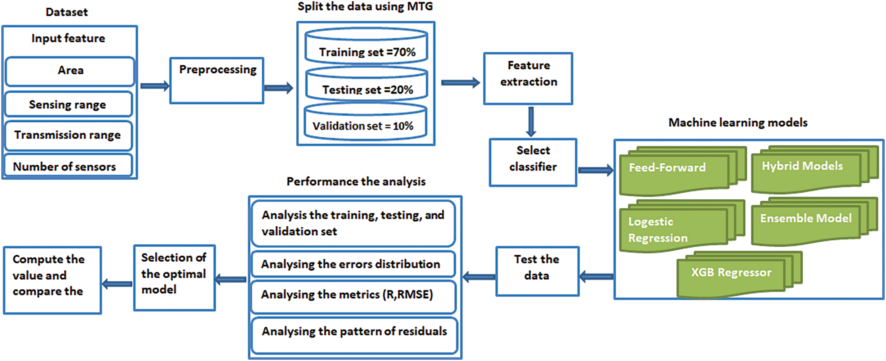
Figure 4: Flowchart representing the system implementation workflow

Generalisability is extensively investigated in WSN intrusion detection machine learning models. K-fold cross-validation segments the data into k “folds.” Validation and model training employ one fold and k − 1 iterations. Repeating this k times trains and validates every data point, decreasing overfitting and boosting model performance on unseen data. By averaging findings over all k iterations, the study reduces dependence on a single train-test split. It boosts confidence in the model’s capacity to generalise to unexpected real-world situations.

Table 4 presents the performance metrics of various machine learning models implemented. The models were evaluated under Gaussian and Uniform sensor distributions using key indicators: Correlation Coefficient (R), RMSE, and the predicted number of barriers. These metrics provide insight into each model’s accuracy, error rate, and ability to partition network traffic effectively. CNN-LSTM and Ensemble models generally show superior performance across both distributions.

6.1 Experimental Results for Gaussian Sensor Distribution

We reported the training, validation, testing, and overall accuracy to assess the performance of the trained neural networks under Gaussian sensor distribution. To assess the training accuracy, we utilized the training dataset as input for the trained models and assessed their performance, yielding the subsequent outcomes: The CNN-LSTM model achieved an R of 0.99 and RMSE of 6.36 on the training dataset, the Ensemble Model achieved an R of 0.99 and an RMSE of 7.19 on the training dataset, the Feedforward ANN model achieved, an R of 0.99 and an RMSE of 9.41 on the training dataset the XGB Regressor model achieved an R of 0.98 and an RMSE of 8.52 on the training dataset. Lastly, the Linear Regression model achieved an R of 0.79 and an RMSE of 31.40 on the training dataset.

We can examine bias by assessing the model’s performance by analyzing the test data. Therefore, it is necessary to evaluate its performance using datasets that have not been previously viewed or used. Firstly, we verified the models using the validation dataset. Each model’s predicted number of barriers (CNN-LSTM, Ensemble Model, Feedforward ANN, XGB Regressor, Linear Regression) were 0.935, 0.883, 0.816, 0.915, and 0.906, respectively. We plotted the cumulative error of each model using a bin size of 20 per model to examine the error distribution during the training, validation, and testing phases. The cumulative error of the trained models, which include CNN-LSTM, ensemble model, feedforward artificial neural network, XGB Regressor, and linear regression, ranges from −10 to 6, −15 to 20, −20 to 40, −10 to 30, and −20 to 100, respectively. The distribution is Gaussian, with a slight rightward skew. The peak of the distribution is near the zero error line, indicating that the model is more accurate. The region indicates the overestimated region to the left of the zero error line. In contrast, the region represents the underestimated region to the right. The trained model generally overestimates the predicted values since the number of cases in the overestimated region is greater than those in the underestimated region.

The error distribution plots for Gaussian and Uniform distributions of the models provide a visual representation of how well each machine learning model performs in predicting the number of barriers in a wireless sensor network. They highlight the models’ strengths and weaknesses.

Fig. 5A–E presents the error distribution for models under Gaussian conditions. Each plot shows how the predicted values deviate from the actual values, with the error values typically ranging from negative to positive.

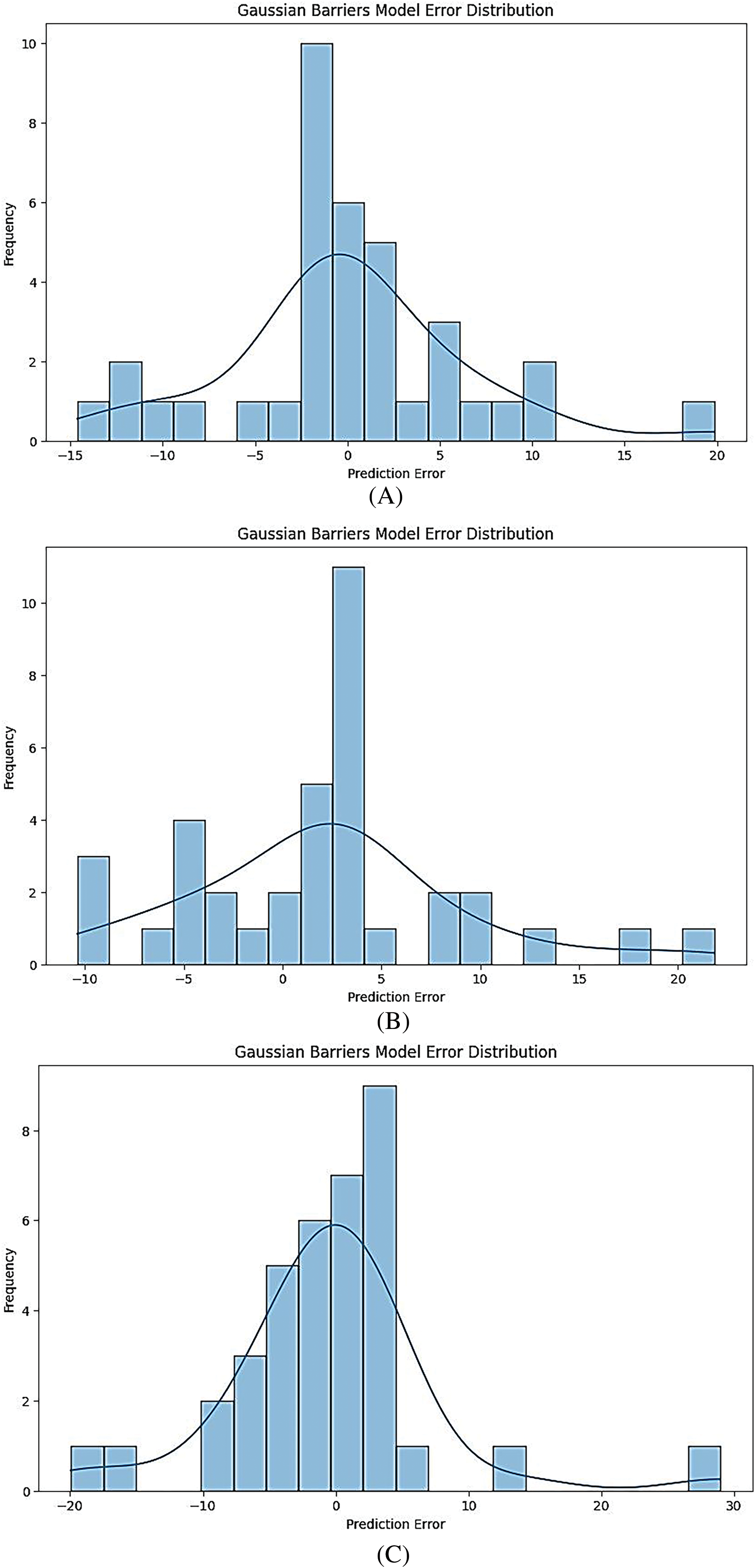
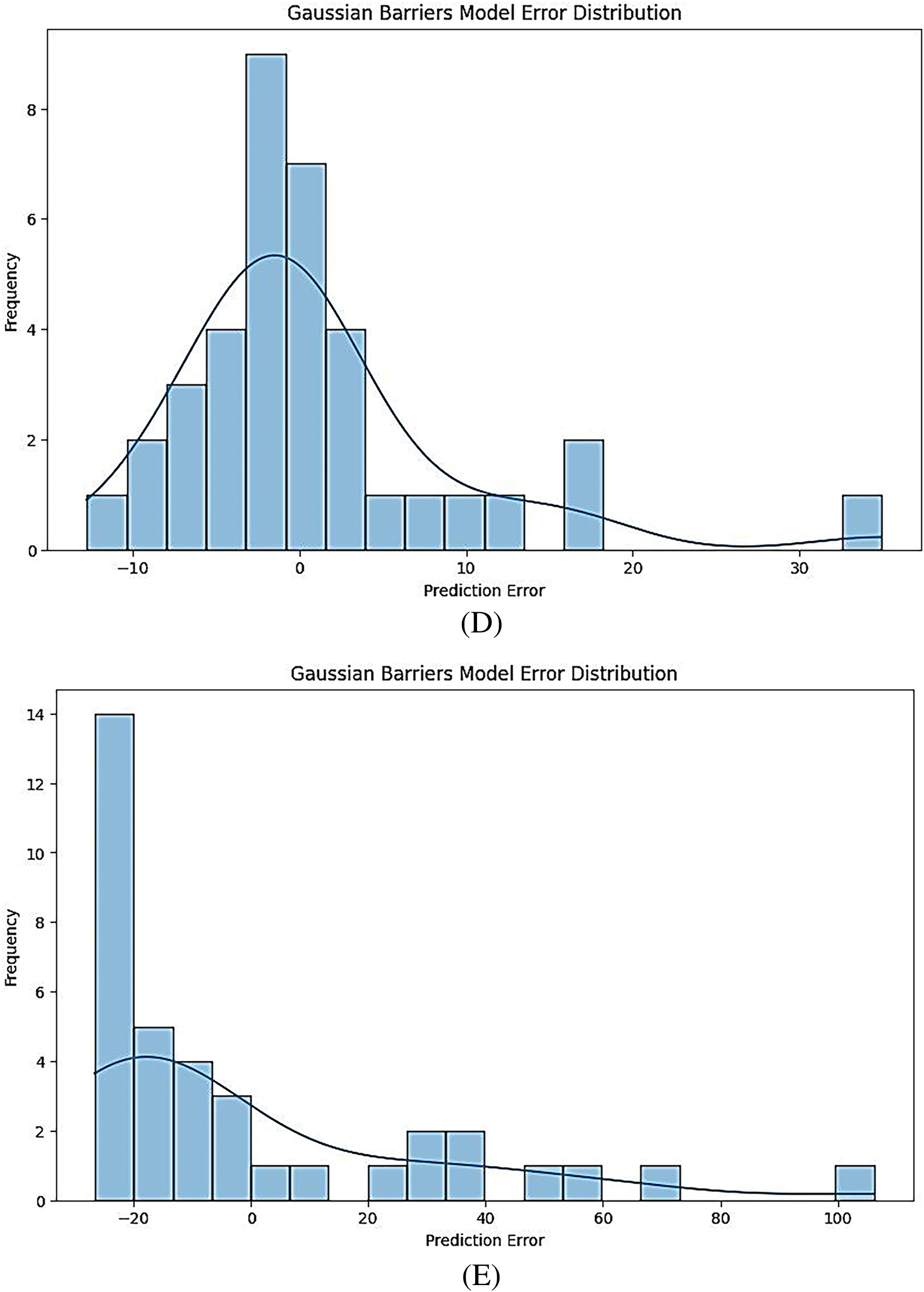
Figure 5: (A) Gaussian barrier models error distribution for CNN-LSTM model. (B) Gaussian barrier models error distribution for ensemble model. (C) Gaussian barrier models error distribution for feed-forward ANN model. (D) Gaussian barrier models error distribution for XGB regressor model. (E) Gaussian barrier models error distribution for linear regression model

For instance, the CNN-LSTM model (Fig. 5A) may show a tighter clustering of errors around zero, indicating better predictive accuracy. In contrast, models like Linear Regression (Fig. 5E) might exhibit a wider spread of errors, suggesting less accuracy in predictions.

6.2 Experimental Results for Uniform Sensor

In addition to assessing the models’ performance in scenarios with Gaussian sensor distribution, we have also tested their performance in scenarios with uniform sensor distribution. We assessed the performance of the trained models under uniform sensor distribution by reporting the accuracy for training, validation, testing, and overall. To evaluate the training accuracy, we used the training dataset as input for the trained models and analysed their performance, resulting in the following outcomes: The CNN-LSTM model achieved an R of 0.98 and an RMSE of 8.51 on the training dataset, the Ensemble Model earned an R of 0.99 and an RMSE of 9.28 on the training dataset, the Feedforward ANN model achieved an R of 0.98 and an RMSE of 16.10 on the training dataset, the XGB Regressor model attained an R of 0.98 and an RMSE of 11.27 on the training dataset. In contrast, the Linear Regression model achieved an R of 0.79 and an RMSE of 37.71 on the same training dataset.

By studying the test data and evaluating the model’s performance, we can look at the predicted number of barriers (Uniform), and we used the validation dataset to ensure that the models were correct. There were 0.981, 0.902, 0.868, 0.919, and 0.932 barriers predicted for the CNN-LSTM, Ensemble Model, Feedforward ANN, XGB Regressor, and Linear Regression models of the machine learning models for this study. During the training, validation, and testing phases, we examined the error distribution by doing an error analysis and plotting the cumulative error of each model using a bin size of 20 per model. The trained models’ cumulative errors vary from −10 to 50 for CNN-LSTM, −20 to 20 for the ensemble model, −20 to 60 for feedforward ANN, −20 to 50 for linear regression, and −25 to 125 for all five models, respectively. There is a small rightward skew in the Uniform distribution. Since the distribution’s peak is close to the zero error line, we can infer that the model provides better results.

Fig. 6A–E depicts the error distribution for the same models under Uniform conditions. Similar to the Gaussian plots, these figures reveal how well the models predict the number of barriers.

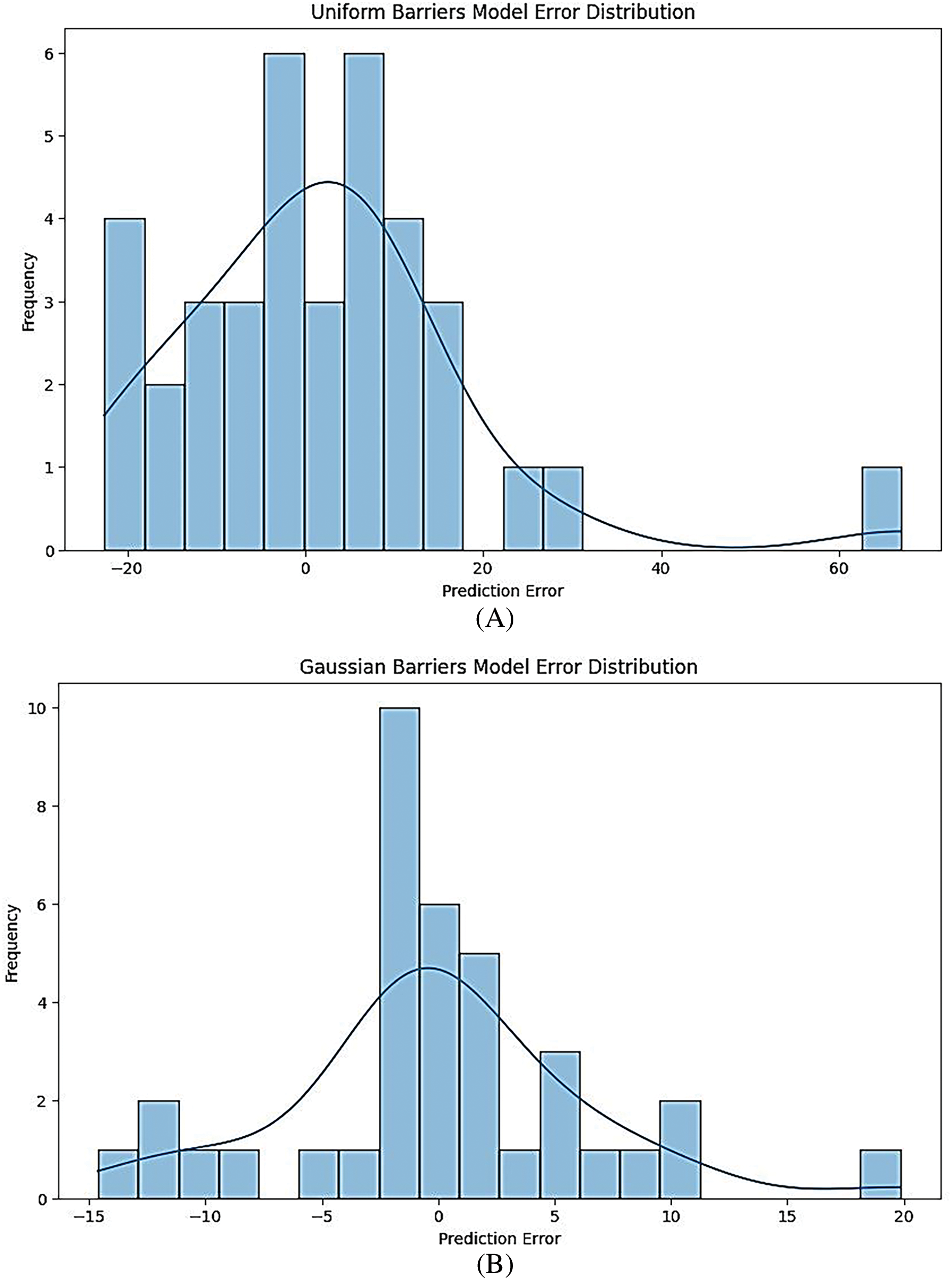
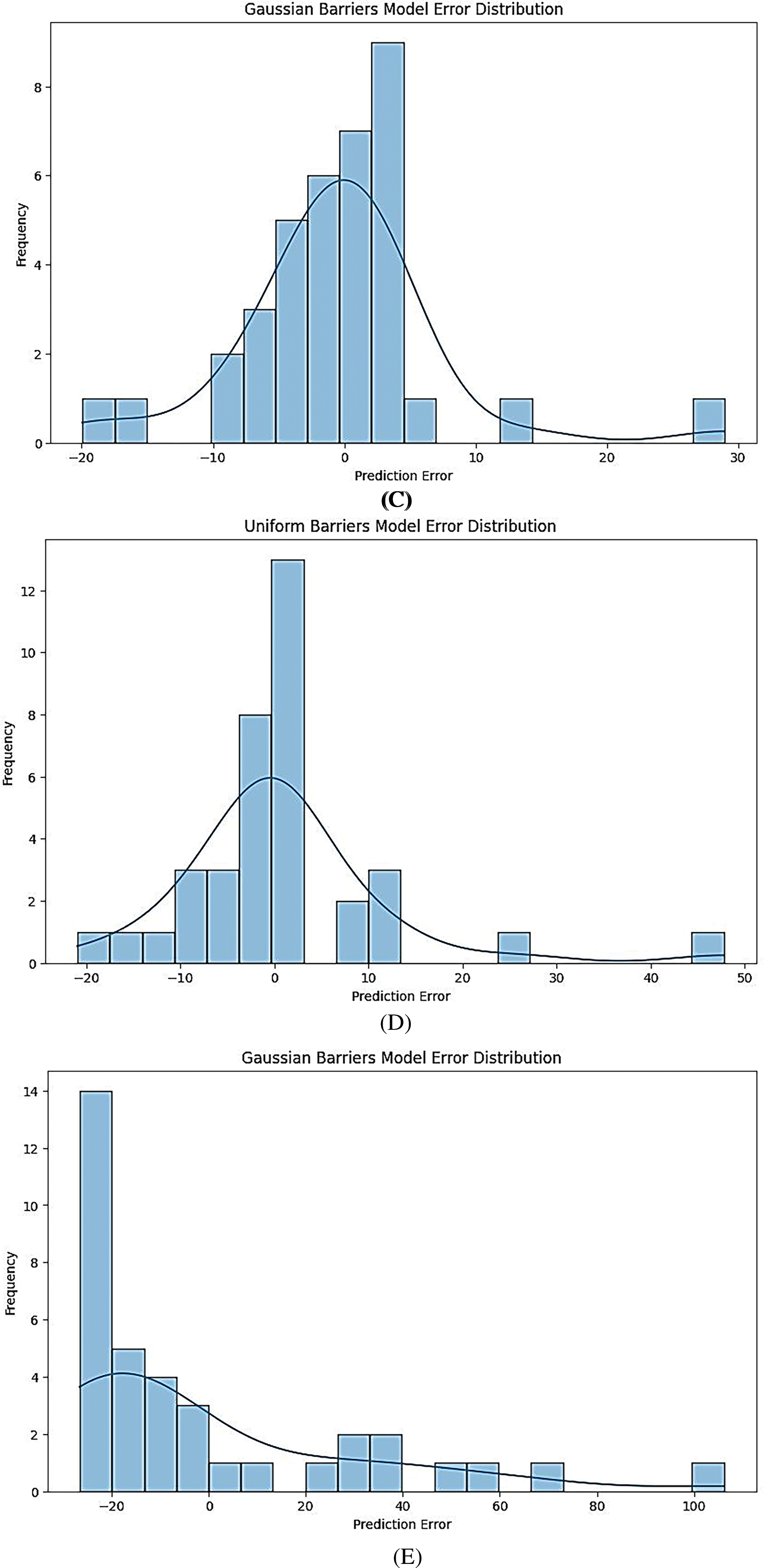
Figure 6: (A) Uniform barrier models error distribution for A; CNN-LSTM model. (B) Uniform barrier models error distribution for ensemble model. (C) Uniform barrier models error distribution for feed-forward ANN model. (D) Uniform barrier models error distribution for XGB regressor model. (E) Uniform barrier models error distribution for linear regression

The uniform distribution plots can show different error characteristics from the Gaussian ones. For example, the Feed-Forward ANN model (Fig. 6C) might demonstrate a different error pattern, potentially indicating that it handles Uniform distributions differently than Gaussian ones.

Fig. 7 presents an analysis of the probability density functions of Gaussian and uniform distributions, especially in the context of different machine learning models, including CNN-LSTM, feedforward artificial neural networks (ANN), XGB Regressor, and linear regression. It is seen how these distributions affect model performance and prediction accuracy. Examining the properties of Gaussian and uniform distributions illustrates the results through comparative visualization.

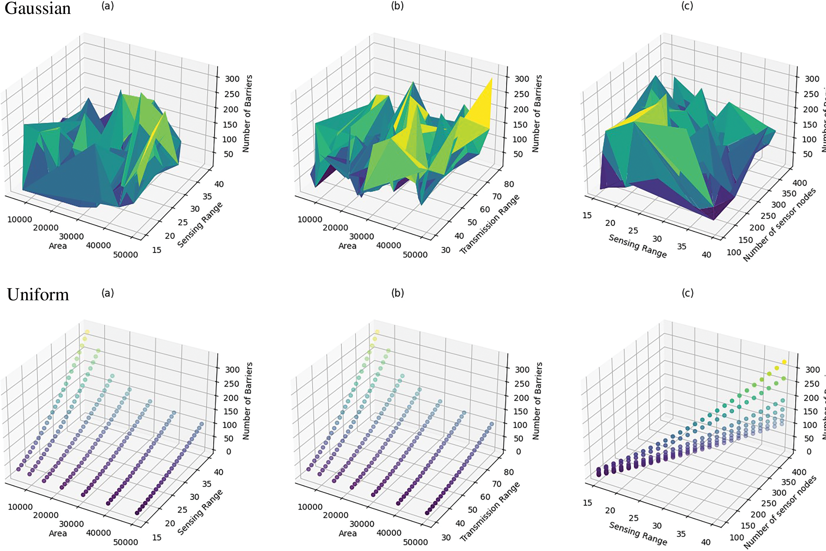
Figure 7: Partial dependence plots (PDPs) of gaussian and uniform for the models: CNN-LSTM, feed-forward ANN, XGB regressor and linear regression. Subfigures a, b, and c show the accuracy of the Ensemble Model, Feed-Forward ANN Model, and Linear Regression Model, respectively, illustrating their varying effectiveness in predictions

6.3 Feature Sensitivity Curve

In order to examine the sensitivity of the features, we created a 2D plot showing the distribution of the features with an axis-aligned histogram and a Partial Dependence Plot (PDP) surface plot that took into account both features simultaneously, along with the confusion matrix.

We found that the number of barriers is negatively correlated with the area of the circular zone. On the other hand, the amount of barriers is positively impacted by the detecting range, transmission range, and sensor count. Due to variations in the outputs of machine learning models and the predictive nature of the dataset used for training, we conducted experiments with hybrid CNN-LSTM models and feedforward ANN networks. As a consequence of this, we were able to obtain a graph that depicted the barrier model loss for both Gaussian and uniform distributions. We generally observed a consistent pattern, with only slight variations in the numbers for all PDPs.

The plots of Gaussian barrier models showing predicted vs. actual values for various machine learning models provide a visual comparison of how accurately each model predicts the number of barriers in a wireless sensor network. Here’s a brief overview of these plots:

•   CNN-LSTM Model:

This plot typically shows a close alignment between predicted and actual values, indicating high accuracy in predictions. The points are clustered around the diagonal line, suggesting that the model effectively captures the underlying data patterns (Figs. 8 and 9).

Figure 8: Gaussian barriers models predicted vs. actual values for the CNN-LSTM model

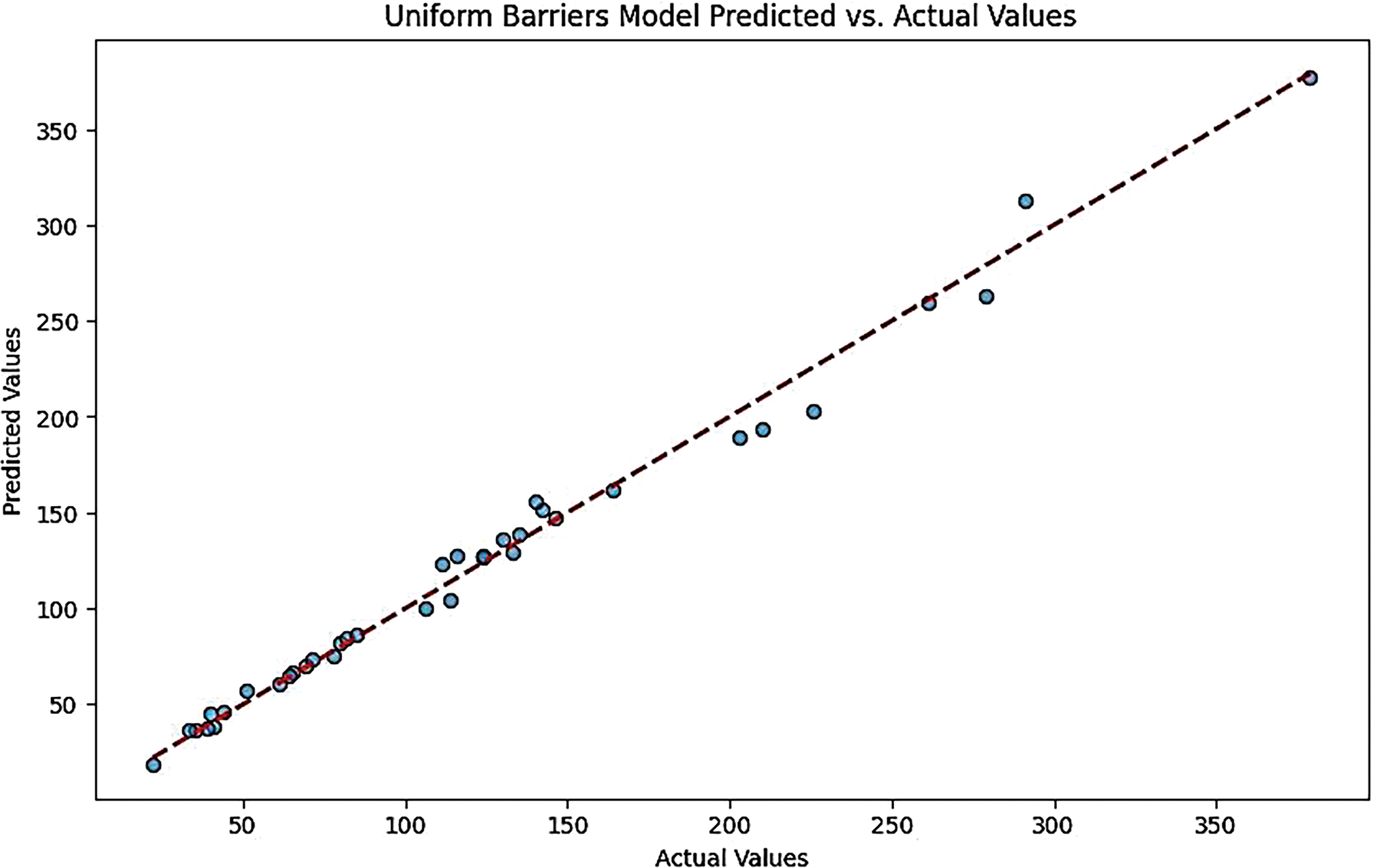
Figure 9: Uniform barriers models predicted vs. actual values for CNN-LSTM model

•   Ensemble Model:

Like the CNN-LSTM, the Ensemble Model’s plot demonstrates a good fit, with predicted values closely following the actual values. This indicates that the ensemble approach effectively combines multiple models to enhance prediction accuracy (Figs. 10 and 11).

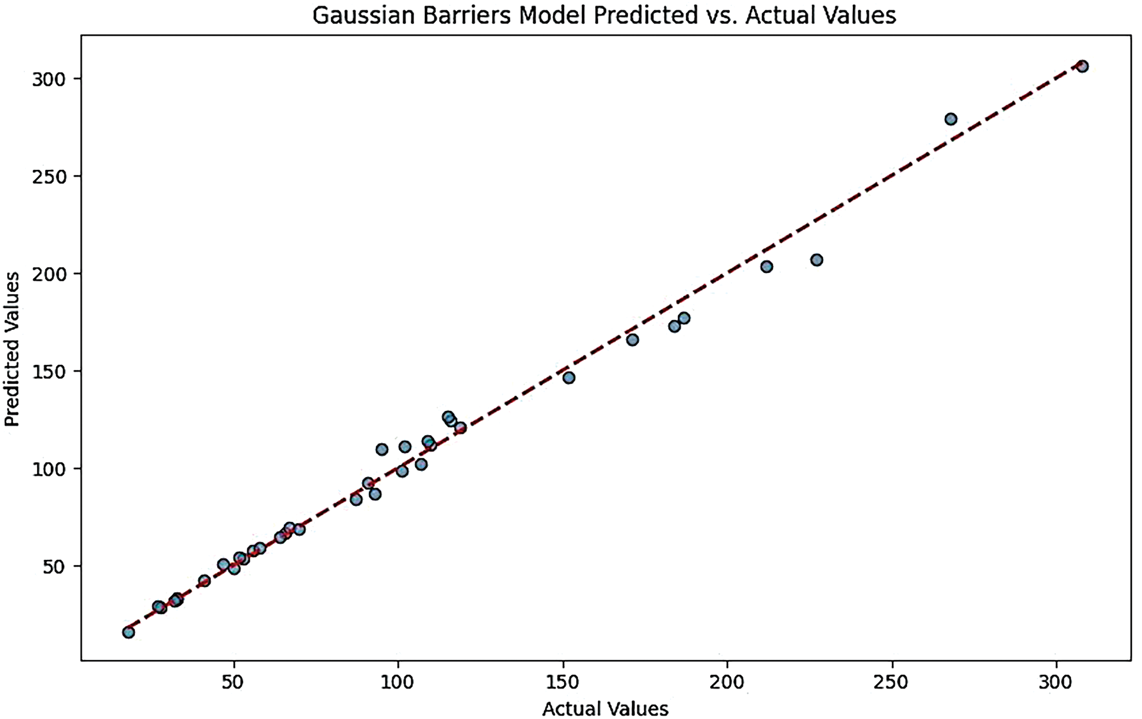
Figure 10: Gaussian barriers models predicted vs. actual values for the ensemble model

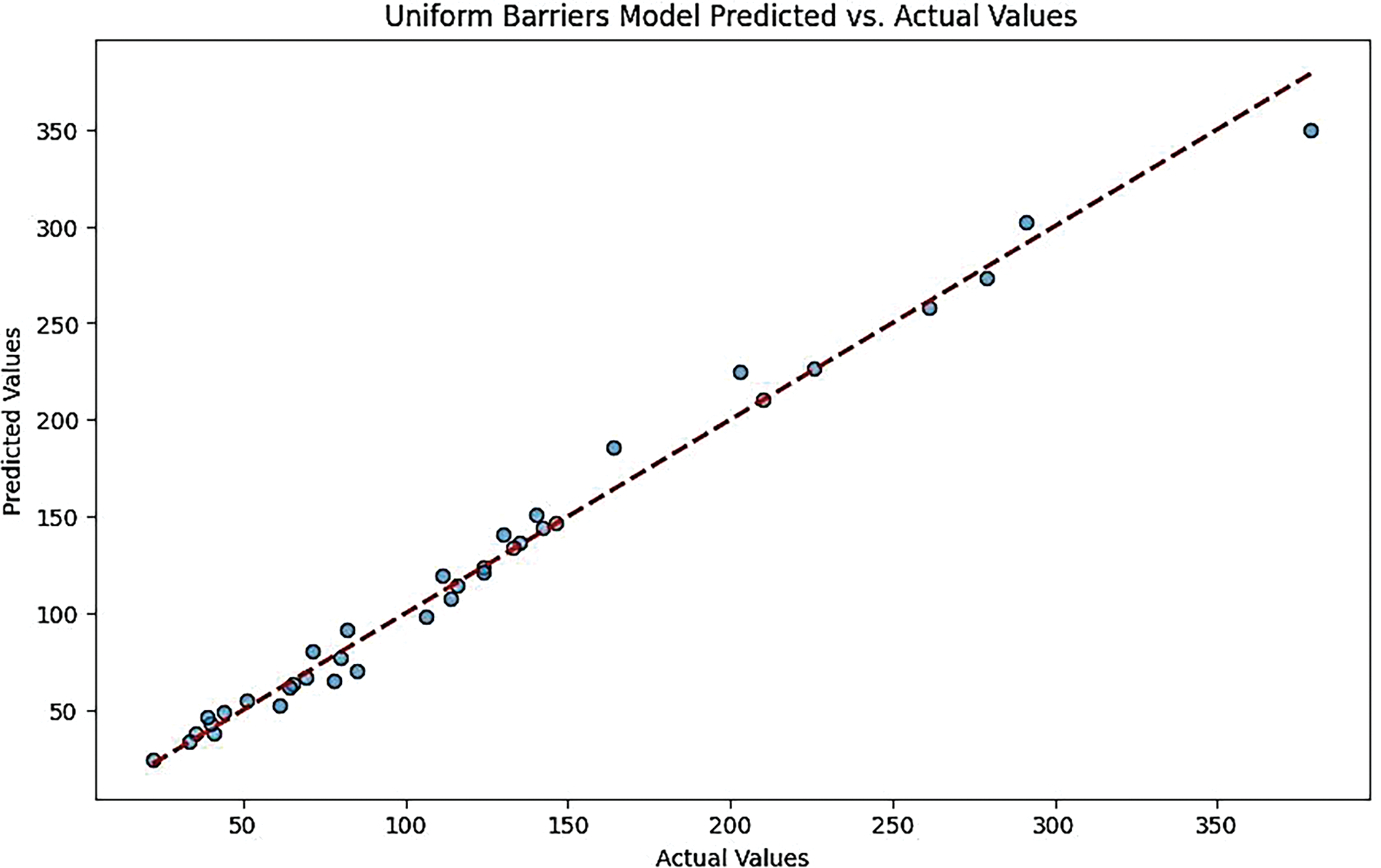
Figure 11: Uniform barriers models predicted vs. actual values for ensemble model

•   Feed-Forward ANN Model:

The plot may show deviations from the diagonal line, indicating moderate accuracy. While the model performs reasonably well, there may be larger prediction errors than the previous models (Figs. 12 and 13).

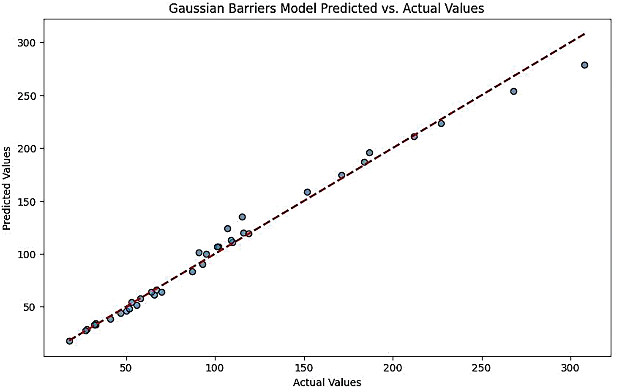
Figure 12: Gaussian barriers models predicted vs. actual values for feed-forward ANN model

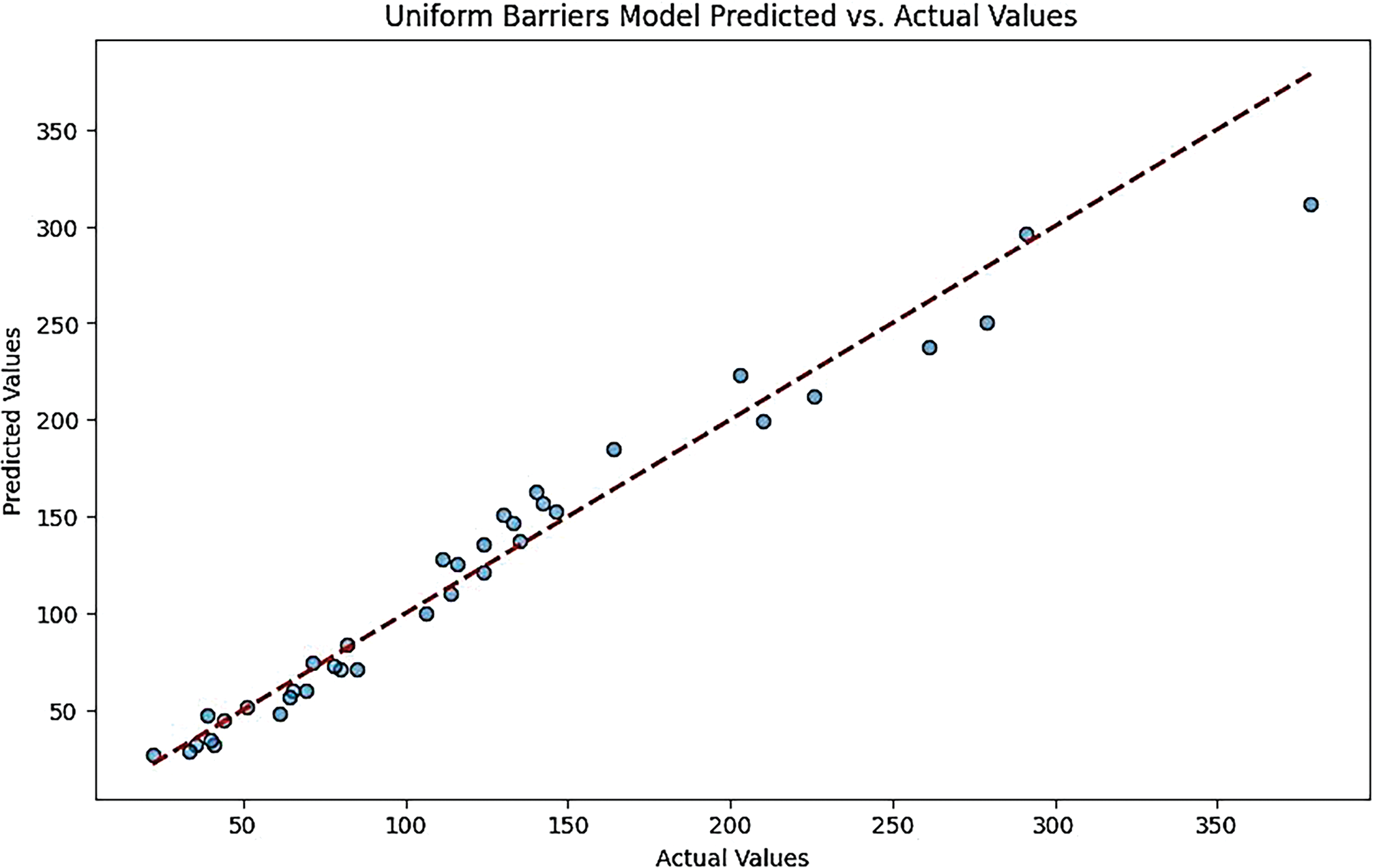
Figure 13: Uniform barriers models predicted vs. actual values for feed-forward ANN model

•   XGB Regressor Model:

This plot often reflects a strong predictive performance, with most points lying close to the diagonal. However, there may be occasional outliers, suggesting that while the model is generally effective, it can struggle with certain data points (Figs. 14 and 15).

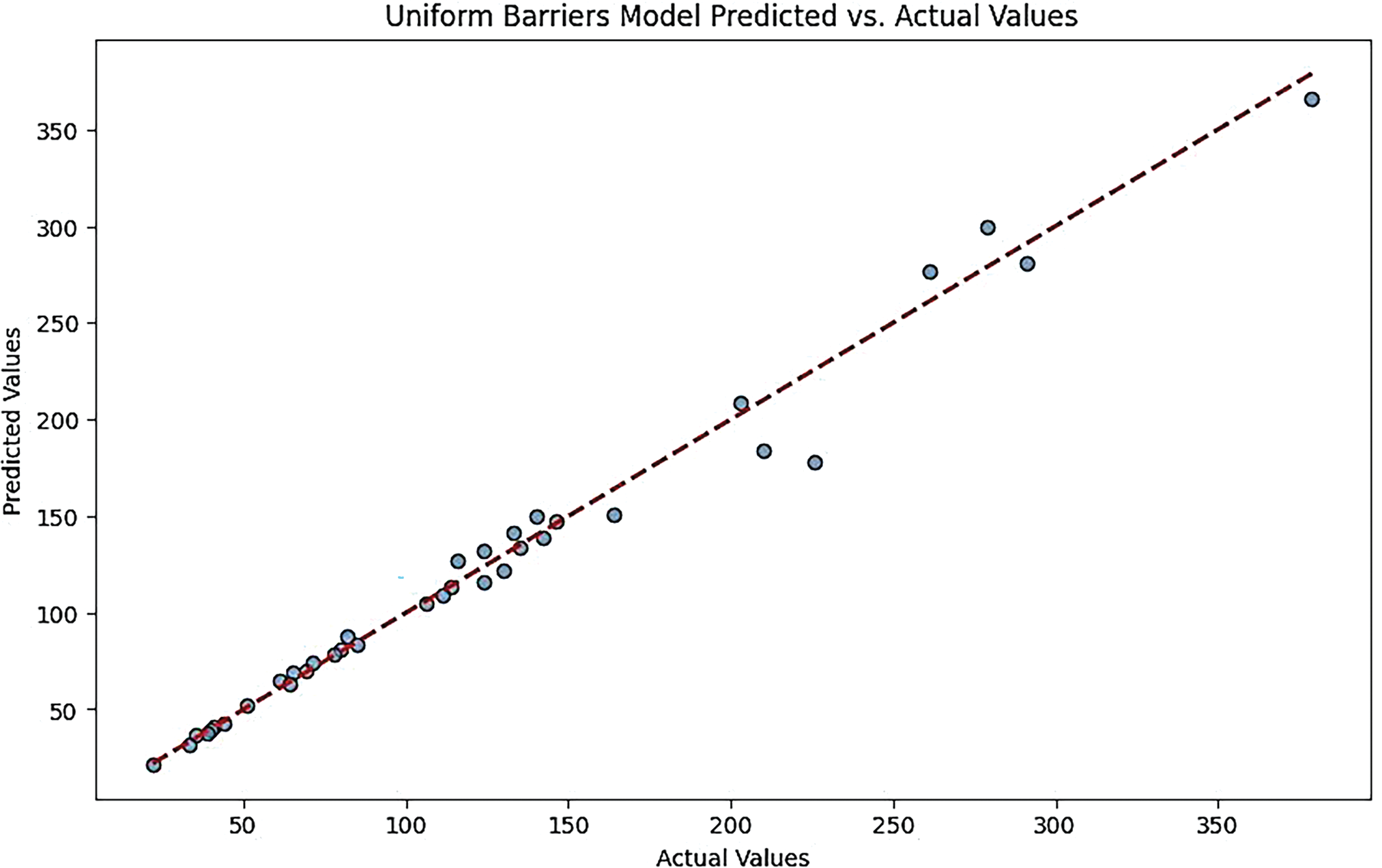
Figure 14: Gaussian barriers models predicted vs. actual values for the XGB regressor model

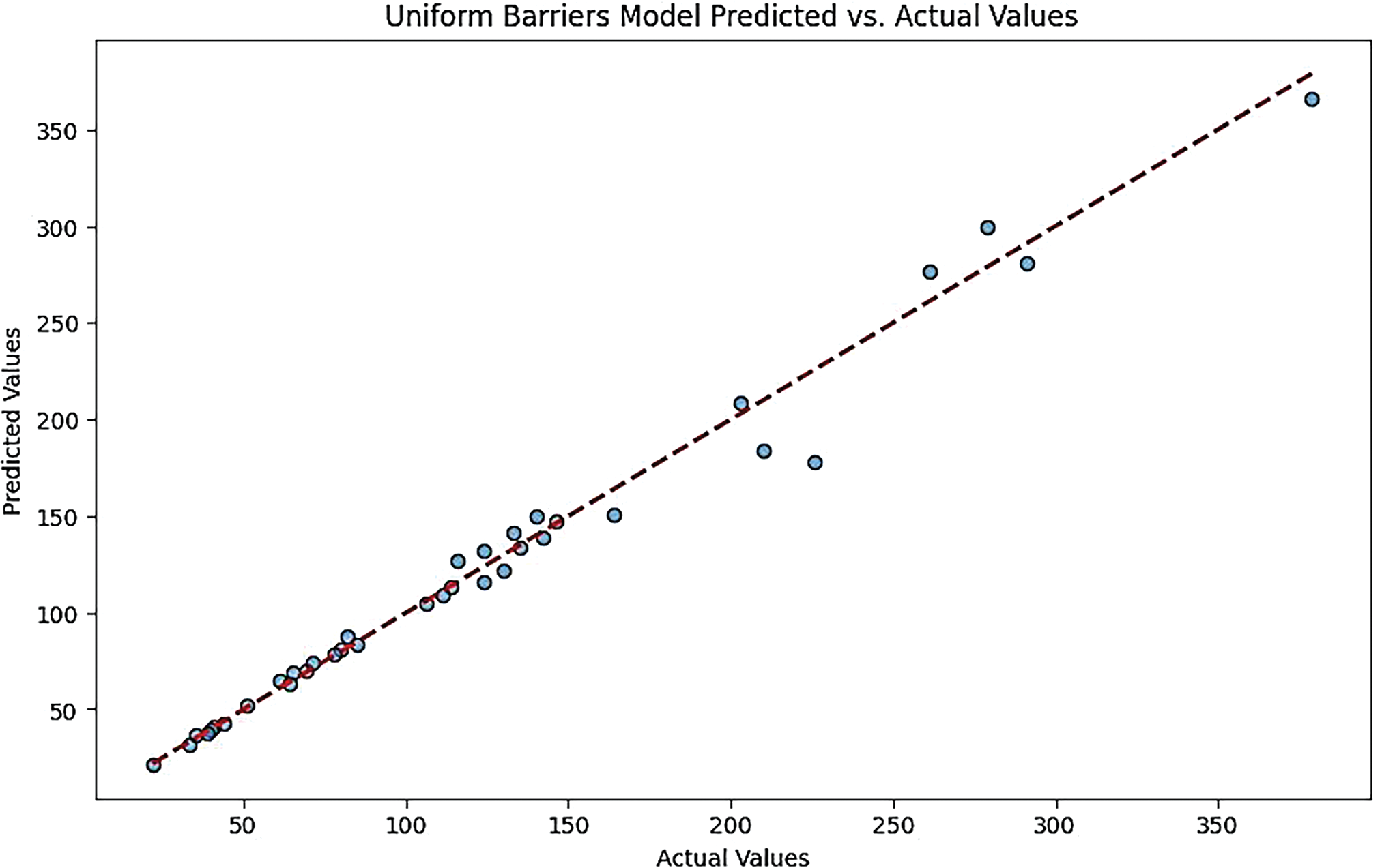
Figure 15: Uniform barriers models predicted vs. actual values for XGB regressor model

•   Linear Regression Model:

The plot for the Linear Regression model may show a wider spread of points away from the diagonal line, indicating lower accuracy in predictions. This suggests that the model may not capture the complexities of the data as effectively as the other models.

In summary, these plots collectively illustrate the predictive performance of each model under Gaussian conditions, highlighting the strengths and weaknesses in their ability to accurately predict the number of barriers (Figs. 16 and 17).

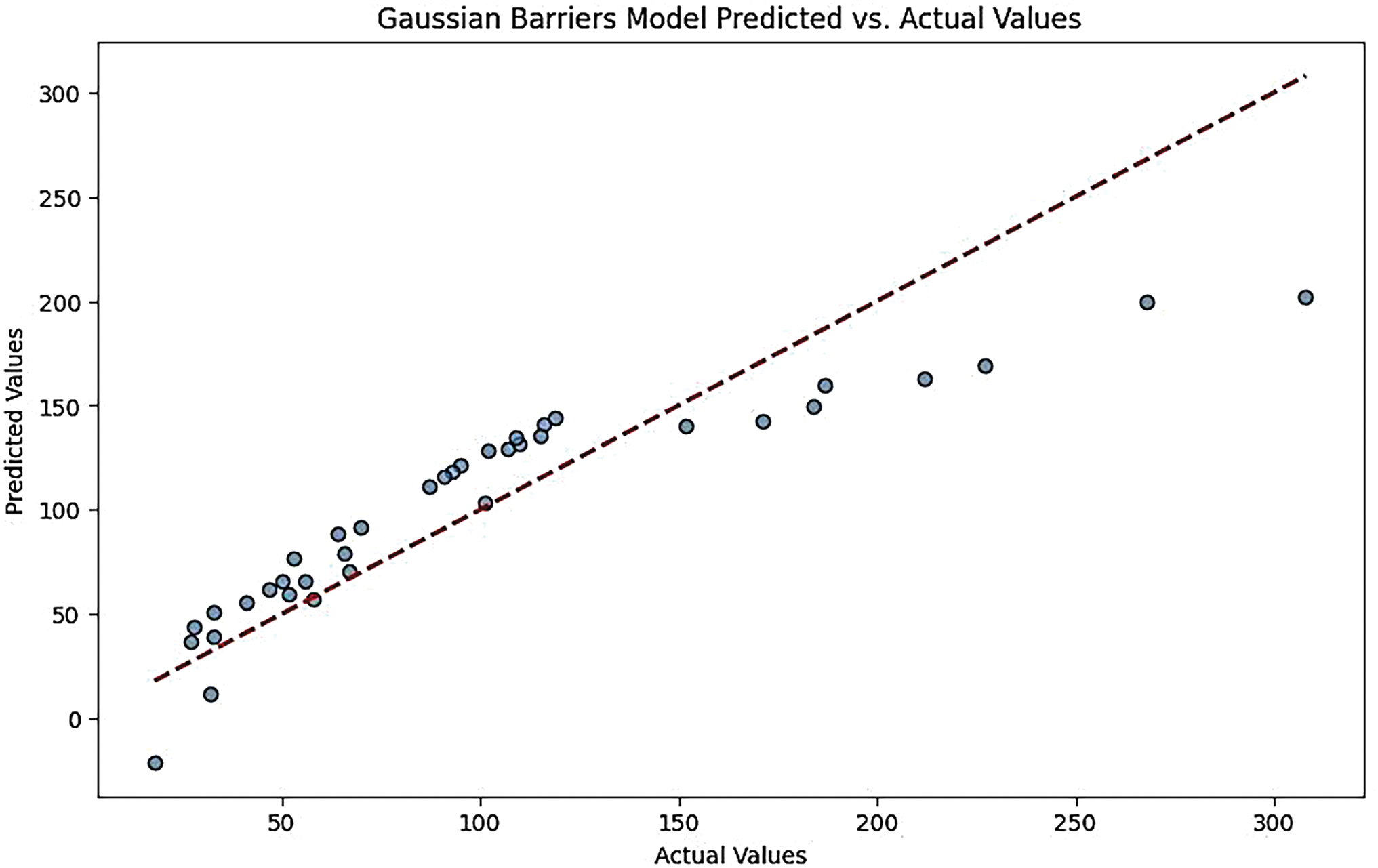
Figure 16: Gaussian barriers models predicted vs. actual values for linear regression model

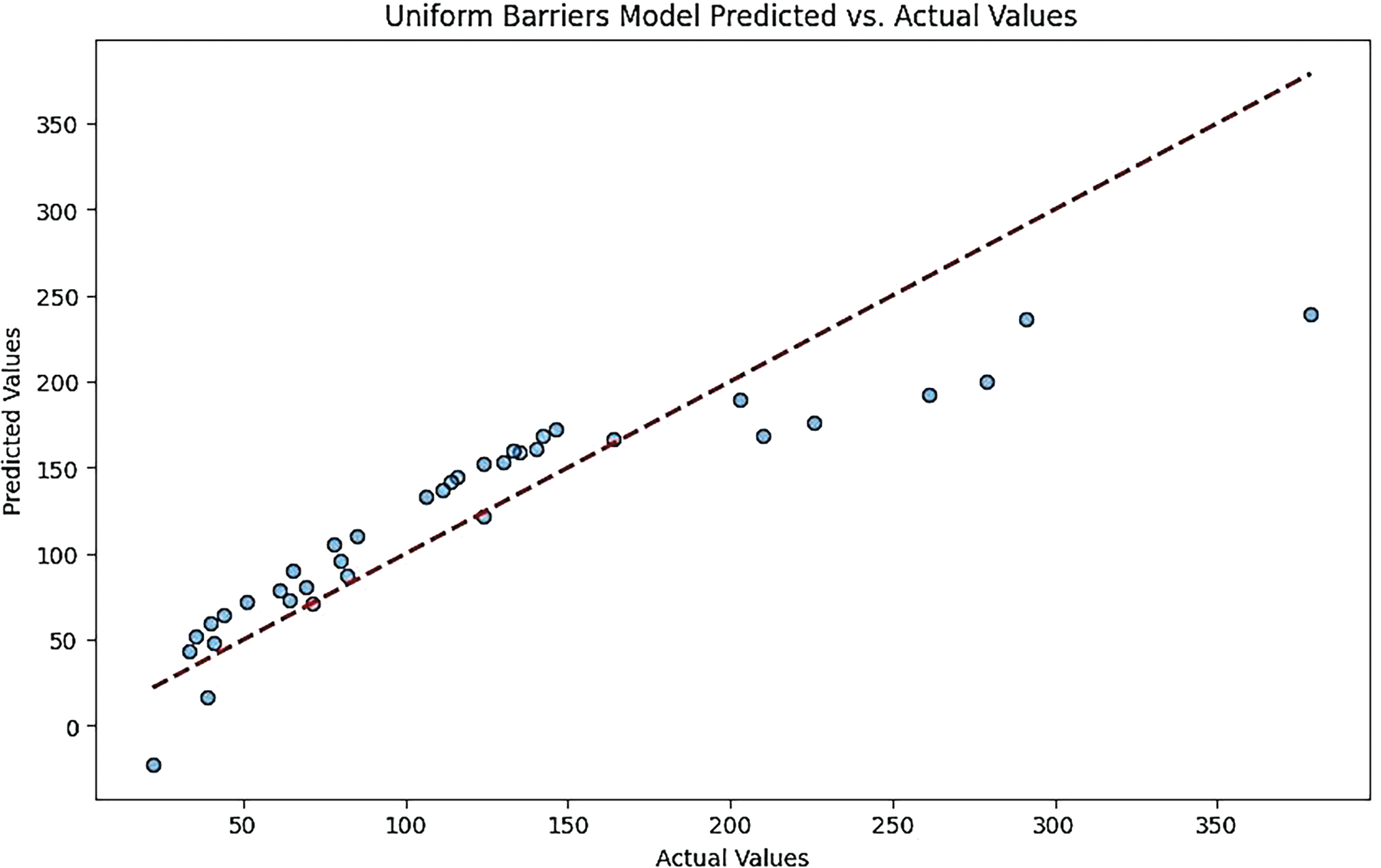
Figure 17: Uniform barriers models predicted vs. actual values for linear regression model

•   Comparative Analysis:

The comparison between Gaussian and Uniform error distributions allows for assessing each model’s robustness across different traffic patterns. For instance, if a model performs well under Gaussian distribution but poorly under Uniform distribution, it may indicate that the model is sensitive to the underlying data distribution.

The cumulative error ranges for each model also provide insights into their performance. For example, the CNN-LSTM model could have a cumulative error range of −10 to 50. In contrast, the Linear Regression model could range from −25 to 125, indicating that the latter has a wider error margin and potentially less reliability.

Fig. 18 shows plots of Gaussian barrier models error distribution values for CNN-LSTM, Ensemble Model, Feed-Forward ANN, XGB Regressor, and Linear Regression model.

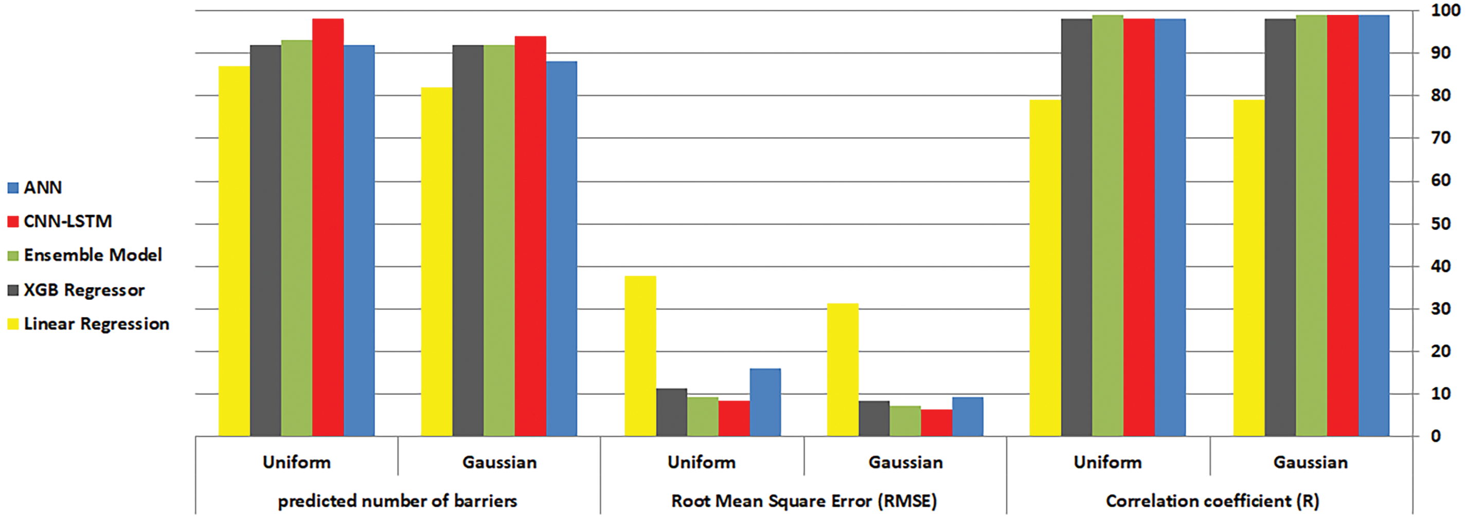
Figure 18: Graphical depiction of evaluation outcomes utilising gaussian and uniform distributions

7  Discussion

This study uses machine learning algorithms to predict the number of barriers in intrusion detection within wireless sensor networks (WSNs). We trained five models for scenarios involving Gaussian and uniform sensor distributions. The correlation coefficient and RMSE are superior in Gaussian and Uniform sensor distribution scenarios.

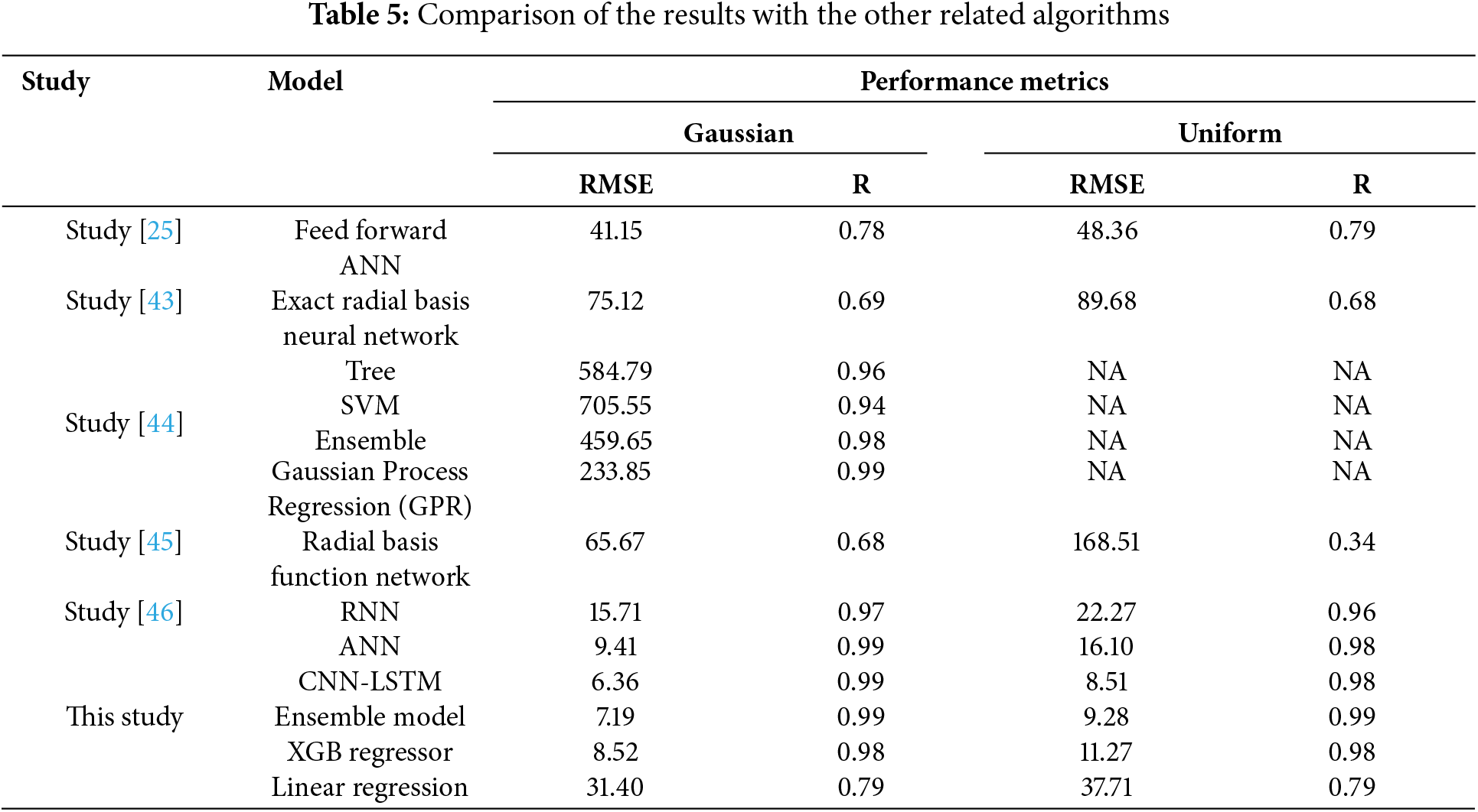
Table 5 demonstrates the superior performance of the predicted number of barriers compared to other models, as shown by the experimental results of the CNN-LSTM model. This study investigated an inclusive barrier-based strategy concerning intrusion detection in wireless sensor networks using various machine-learning models implemented in TensorFlow. Such things as the dynamic visualization possibilities by TensorBoard and the continuous development supported by Google enhanced TensorFlow’s advantages, which made it suitable for this research. This work was mainly devoted to evaluating how well different machine learning models could predict the number of barriers in intrusion detection scenarios that involve Gaussian and Uniform sensor distributions.

In the context of intrusion detection in Wireless Sensor Networks, features like area size, sensing range, communication range, and sensor count are crucial as they directly impact the network’s ability to detect and respond to intrusions. Area size determines the spatial scope, sensing range influences the detection coverage, communication range affects data transmission and sensor connectivity, and sensor count influences network density and robustness, all of which are key to optimizing the accuracy and efficiency of the machine learning model for intrusion detection [38–40].

In order to predict accurately the number of barriers in a wireless network containing Gaussian and uniform sensor distributions, we have employed machine learning tools and ensemble techniques.

One key strength of this work is that it critically assesses all models across training, validation, and testing datasets, unlike similar works [40–42]. They report on R-values and RMSE for each model they test, which are clear quantitative performance measures.

Regarding Gaussian sensor distributions, the CNN-LSTM model is outstanding with an R-value of 0.99 and RMSE value of 6.36, which are better than other models, including feedforward ANN, XGB Regressor, and linear regression. Similarly, for Uniform Sensor Distributions, the CNN-LSTM model shows an R of 0.98 and RMSE of 8.51, thus proving its superior ability to predict.

The accuracy was assessed by checking how well the models worked on each phase (training, validation, testing) regarding Gaussian sensor distribution used as an experimental setup. CNN-LSTM performed better with the train data set, scoring an R of 0.99 and an RMSE of 6.36. The ensemble model also did well, having an R-value or coefficient equal to that for CNN-LSTM but different RNSE = 7.19. The Feedforward ANN got as high as R = 0.99 while RMSE = 9.41 compared to XGB Regressor’s R = 0.98 and RMSE = 8.52.The linear regression model lags with only 0.79 for the R-value, but huge mistakes will be predicted; this can be seen from its grossly higher RMSE. The validation set reiterated these results wherein CNN-LSTM & Ensemble were more accurate in predicting the number of barriers than other models.

The inclusion of simpler models like linear regression alongside more complex ones, such as CNN-LSTM, raises questions about their specific role in the study. Linear regression serve as a baseline or control model, providing a straightforward comparison point for evaluating the performance gains achieved by more advanced machine learning techniques. By contrasting the accuracy and robustness of complex and simple models, the study can better illustrate the effectiveness of CNN-LSTM and other sophisticated approaches in handling imbalanced data and detecting intrusions in Wireless Sensor Networks.

The error analysis further reveals how the models performed under Gaussian distribution. Cumulative error plots indicated that CNN-LSTM had the narrowest errors, implying it was highly accurate. Similarly, Ensemble and XGB Regressor models exhibited relatively close error distributions. On the other hand, Feedforward ANN and Linear Regression models had wider error distributions, meaning poor precision. In all models, the distribution of errors was slightly skewed to the right side, with its peak near the zero-error line, indicating that generally overestimated barrier numbers. The uniform sensor distribution scenario showed similar trends in this regard. For the training dataset, the CNN-LSTM model had an R-value of 0.98 and an RMSE value of 8.51, showing a slightly poorer but acceptable performance compared to the Gaussian scenarios. An R factor of 0.99 and an RMSE for the ensemble model were recorded at 9.28, highlighting a good performance while carrying out this study on the training data set using the BARRIERS dataset instead of a barriers.csv data file, which could have been used during the preprocessing phase conducted on a related research project by our team. With an R coefficient of 0.98 as well as an RMSE equal to 16.10, for instance, represents what we found when trying to simulate a feedforward neural network for use within this work, whereas XGB regressor gave us back R having value around 0 with its root mean square deviation being approximately 11% higher than that from any other mentioned approach there also exist another option called data miner which is often used times while searching through vast amounts unstructured information about people who are likely targets such as (students who regularly attend school); In terms of accuracy or closeness accuracy, values from the linear regression model were given by R = 0.79, with RMSE = 37.71, making it the worst performer among all these five methods tested in our experiments.

The validation results further supported these findings, where the CNN-LSTM model provided the most accurate predictions, followed by the Ensemble and XGB Regressor models. The error analysis of the Uniform distribution showed a similar trend to the Gaussian distribution, where the CNN-LSTM model had the narrowest error distribution. While feedforward ANN and linear regression models exhibited wider error distributions, ensemble, and XGB regressor models showed relatively tight errors.

The sensing range was the most important feature in predicting the number of barriers, which showed a positive correlation with the number of barriers. In addition, the transmission range and number of sensors were also of great importance, indicating that the greater the sensing and transmission capabilities, the greater the number of barriers needed to effectively manage the traffic in the network. The results also showed an inverse relationship between the number of barriers and the size of the circular area, indicating that larger areas may require fewer barriers, which may result from the increased coverage provided by each sensor in large areas.

As sensitivity plots indicated almost similar patterns among different models, their robustness was confirmed in cases of both CNN-LSTM and Ensemble. Next, comparing these outcomes with other relevant studies shows that CNN-LSTM and Ensemble are more effective in predicting WSN intrusion detection scenarios’ barrier numbers than any other methods available in the literature. The best-performing model by [43] in intrusion detection for WSNs using ML had an R of 0.69 and RMSE of 75.12 under Gaussian distribution were not as accurate as our CNN-LSTM model. Similarly, in [44–46], their hybrid neural networks for WSN security indicated a better performance with R and RMSE under Uniform distribution. A study [25] on learning models for WSNs showed that the best ensemble model had a Gaussian R–value of 0.78 and an RMSE value of 41.15. In contrast, our Ensemble Model achieved an even higher R-value of 0.99 with an RMSE value of 7.19.

Overall, Gaussian and Uniform distributions demonstrated strong performances from the CNN-LSTM and Ensemble models throughout this research, indicating their resiliency and reliability.

They can be used in various WSN scenarios since they both attain low RMSE values and preserve high correlation coefficients, even when the sensors are distributed differently. The improved performance is due to the intricate architecture of the CNN-LSTM model that incorporates components from convolutional neural networks (CNNs) and long short-term memory (LSTM) networks, thus efficiently capturing spatial and temporal dependencies. The Ensemble Model benefits from combining multiple models, leveraging their strengths to achieve better overall performance.

The barrier-based approach for intrusion detection in Wireless Sensor Networks (WSNs) has significant real-world implications across various applications:

•   Military Applications: Enhances security in surveillance and reconnaissance, protecting sensitive data and operational integrity.

•   Environmental Monitoring: Safeguards networks that collect critical environmental data, ensuring reliability and accuracy in monitoring.

•   Healthcare: Protects patient monitoring systems and medical devices, maintaining data integrity and patient privacy.

•   Smart Agriculture: Secures networks monitoring soil and crop conditions, leading to better resource management and optimisation of yield.

•   Industrial Automation: Enhances the security of networks monitoring industrial processes, preventing unauthorized access and ensuring safety.

•   Urban Infrastructure: Supports smart city applications by securing traffic management and public safety networks, enhancing overall public safety.

In summary, the five selected models in this study were chosen to address issues such as imbalanced data, the need for accurate predictions, and the ability to capture complex patterns in network traffic. The hybrid CNN-LSTM model, in particular, was highlighted for its capability to analyze temporal patterns, making it well-suited for detecting anomalies in evolving attack scenarios.

To address the limitations in Future work by exploring additional machine learning techniques, particularly transformer-based models. These models can improve detection accuracy and adaptability in intrusion detection systems, enabling better handling of complex and evolving attack patterns in Wireless Sensor Networks (WSNs). This exploration could lead to more effective and resilient security solutions tailored to the unique challenges faced by WSNs.

8  Conclusion

This study introduced the structure of five machine-learning neural network models for precisely determining the number of obstacles in wireless sensor networks for intrusion detection. We trained the Gaussian and uniform sensor distribution models using four possible features retrieved through simulation. During the evaluation of feature importance and sensitivity in the Gaussian and uniform sensor distribution scenario, we found that the sensing range, transmission range, and number of sensors are the most significant features. These features have a beneficial impact on the prediction. Conversely, the area is the least significant characteristic and negatively correlates with the forecast. Upon completing the training of the models, we assessed their performance using data that had not been previously observed. Our evaluation revealed that both the CNN-LSTM and Ensemble models outperformed the others and exhibited promising outcomes. Our methodology can be employed to decrease the cost prerequisites and time during the practical establishment of networks.

For future research, incorporating contextual features like environmental factors (e.g., humidity and temperature) and network load could enhance intrusion detection in Wireless Sensor Networks. These elements may affect sensor accuracy and network stability, offering valuable data that could improve model adaptability and predictive performance, particularly in dynamic, real-world environments.

Acknowledgement: I would like to express my heartfelt gratitude to all those who assisted me in the completion of this research, particularly my colleagues in the teaching and administrative staff at Al-Ain University in Nasiriyah, Thi Qar University, and Babylon University for their exceptional support, which provided the author with crucial knowledge and comprehension of the research.

Funding Statement: The authors received no specific funding for this study.

Author Contributions: The authors confirm their contributions to the paper as follows: study conception and design: Haydar Abdulameer Marhoon, Rafid Sagban; data collection: Haydar Abdulameer Marhoon, Rafid Sagban; analysis and interpretation of results: Haydar Abdulameer Marhoon, Rafid Sagban; draft manuscript preparation: Atheer Y. Oudah, Saadaldeen Rashid Ahmed. All authors reviewed the results and approved the final version of the manuscript.

Availability of Data and Materials: The datasets generated and analyzed during the current study can be downloaded from https://www.kaggle.com/datasets/abhilashdata/ffannid-intrusion-detection-in-wsns/data, and the code can be downloaded from https://in.mathworks.com/matlabcentral/fileexchange/116670-a-deep-learning-approach-to-predict-the-number-of-k-barriers?s_tid=prof_contriblank (accessed on 19 July 2024).

Ethics Approval: Not applicable.

Conflicts of Interest: The authors declare no conflicts of interest regarding the present study.

References

1. Kumar A, Sharma S. Participation of 5G with wireless sensor networks in the internet of things (IoT) application. Wirel Sens Netw Internet Things. 2021 Jun;229–44. doi:10.1201/9781003131229-17. [Google Scholar] [CrossRef]

2. Majid M, Habib S, Javed AR, Rizwan M, Srivastava G, Gadekallu TR, et al. Applications of wireless sensor networks and internet of things frameworks in the Industry Revolution 4.0: a systematic literature review. Sensors. 2022 Mar;22(6):2087. doi:10.3390/s22062087. [Google Scholar] [CrossRef]

3. Yang G, Dai L, Wei Z. Challenges, threats, security issues and new trends of underwater wireless sensor networks. Sensors. 2018 Nov;18(11):3907. doi:10.3390/s18113907. [Google Scholar] [CrossRef]

4. Ismail S, Dawoud DW, Reza H. Securing wireless sensor networks using machine learning and blockchain: a review. Future Internet. 2023 May;15(6):200. doi:10.3390/fi15060200. [Google Scholar] [CrossRef]

5. Hu Z, Wang L, Qi L, Li Y, Yang W. A novel wireless network intrusion detection method based on adaptive synthetic sampling and an improved convolutional neural network. IEEE Access. 2020;8:195741–51. doi:10.1109/access.2020.3034015. [Google Scholar] [CrossRef]

6. Odeh A, Abu Taleb A. Ensemble-based deep learning models for enhancing IoT intrusion detection. Appl Sci. 2023 Nov;13(21):11985. doi:10.3390/app132111985. [Google Scholar] [CrossRef]

7. de Campos Souza PV, Lughofer E, Batista HR. An explainable evolving fuzzy neural network to predict the k barriers for intrusion detection using a wireless sensor network. Sensors. 2022;22(14):5446. doi:10.3390/s22145446. [Google Scholar] [CrossRef]

8. Jiang S, Zhao J, Xu X. SLGBM: an intrusion detection mechanism for wireless sensor networks in smart environments. IEEE Access. 2020;8:169548–58. doi:10.1109/ACCESS.2020.3024219. [Google Scholar] [CrossRef]

9. Alekseeva D, Stepanov N, Veprev A, Sharapova A, Lohan ES, Ometov A. Comparison of machine learning techniques applied to traffic prediction of real wireless network. IEEE Access. 2021;9:159495–514. doi:10.1109/ACCESS.2021.3129850. [Google Scholar] [CrossRef]

10. Tama BA, Lim S. Ensemble learning for intrusion detection systems: a systematic mapping study and cross-benchmark evaluation. Comput Sci Rev. 2021 Feb;39(1):100357. doi:10.1016/j.cosrev.2020.100357. [Google Scholar] [CrossRef]

11. Garcia LPF, Rivolli A, Alcoba E, Lorena AC. Boosting meta-learning with simulated data complexity measures. Intell Data Anal. 2020 Sep;24(5):1011–28. doi:10.3233/IDA-194803. [Google Scholar] [CrossRef]

12. Jemili F, Meddeb R, Korbaa O. Intrusion detection based on ensemble learning for big data classification. Cluster Comput. 2023 Nov;27(3):3771–98. doi:10.1007/s10586-023-04168-7. [Google Scholar] [CrossRef]

13. Abdulganiyu OH, Tchakoucht TA, Saheed YK, Ahmed HA. XIDINTFL-VAE: XGBoost-based intrusion detection of imbalance network traffic via class-wise focal loss variational autoencoder. J Supercomput. 2025;81(1):1–38. doi:10.1007/s11227-024-06552-5. [Google Scholar] [CrossRef]

14. Wang W, Zhu Q. Sequential Monte Carlo localization in mobile sensor networks. Wirel Netw. 2007 Sep;15(4):481–95. doi:10.1007/s11276-007-0064-3. [Google Scholar] [CrossRef]

15. Karthikeyan M. Firefly algorithm based WSN-IoT security enhancement with machine learning for intrusion detection. Sci Rep. 2024;14(1):231. [Google Scholar]

16. Sajid M, Malik KR, Almogren A, Malik TS, Khan AH, Tanveer J. Enhancing intrusion detection: a hybrid machine and deep learning approach. J Cloud Comput. 2024;13(1):123. doi:10.1186/s13677-024-00685-x. [Google Scholar] [CrossRef]

17. Maheswari M, Karthika RA. A novel hybrid deep learning framework for intrusion detection systems in WSN-IoT networks. Intell Automat Soft Comput. 2022;33(1):365–82. doi:10.32604/iasc.2022.022259. [Google Scholar] [CrossRef]

18. Sohi SM, Seifert J-P, Ganji F. RNNIDS: enhancing network intrusion detection systems through deep learning. Comput Secur. 2021 Mar;102(3):102151. doi:10.1016/j.cose.2020.102151. [Google Scholar] [CrossRef]

19. Ahmed O. Enhancing intrusion detection in wireless sensor networks through machine learning techniques and context awareness integration. Int J Mathemat, Stat, Comput Sci. 2024;2:244–58. doi:10.59543/ijmscs.v2i.10377. [Google Scholar] [CrossRef]

20. Ramkumar K, Alzubaidi LH, Malathy V, Venkatesh T. Intrusion detection system in wireless sensor networks using modified recurrent neural network with long short-term memory. In: 2024 International Conference on Integrated Circuits and Communication Systems (ICICACS); 2024; IEEE. p. 1–5. doi:10.1109/ICICACS60521.2024.10498333. [Google Scholar] [CrossRef]

21. Alauddin Rezvi M, Moontaha S, Akter Trisha K, Tasnim Cynthia S, Ripon S. Data mining approach to analyzing intrusion detection of wireless sensor network. Indones J Electr Eng Comput Sci. 2021 Jan;21(1):516. doi:10.11591/ijeecs.v21.i1.pp516-523. [Google Scholar] [CrossRef]

22. Abhale AB, Manivannan SS. Supervised machine learning classification algorithmic approach for finding anomaly type of intrusion detection in wireless sensor network. Opt Mem Neural Netw. 2020 Jul;29(3):244–56. doi:10.3103/S1060992X20030029. [Google Scholar] [CrossRef]

23. Alqahtani M, Gumaei A, Mathkour H, Maher Ben Ismail M. A genetic-based extreme gradient boosting model for detecting intrusions in wireless sensor networks. Sensors. 2019 Oct;19(20):4383. doi:10.3390/s19204383. [Google Scholar] [CrossRef]

24. Salmi S, Oughdir L. CNN-LSTM based approach for dos attacks detection in wireless sensor networks. Int J Adv Comput Sci Appl. 2022;13(4). doi:10.14569/issn.2156-5570. [Google Scholar] [CrossRef]

25. Chokkalingam S. Enhancing intrusion detection in wireless sensor networks using deep learning-based K-barriers prediction. In: 2023 International Conference on Self Sustainable Artificial Intelligence Systems (ICSSAS); 2023 Oct; IEEE. p. 1208–15. doi:10.1109/icssas57918.2023.10331818. [Google Scholar] [CrossRef]

26. Lilhore UK, Manoharan P, Simaiya S, Alroobaea R, Alsafyani M, Baqasah AM, et al. HIDM: hybrid intrusion detection model for Industry 4.0 networks using an optimized CNN-LSTM with transfer learning. Sensors. 2023 Sep;23(18):7856. doi:10.3390/s23187856. [Google Scholar] [CrossRef]

27. Sedhuramalingam K, Saravanakumar N. A novel optimal deep learning approach for designing intrusion detection system in wireless sensor networks. Egypt Inform J. 2024;27(3):100522. doi:10.1016/j.eij.2024.100522. [Google Scholar] [CrossRef]

28. Muruganandam S, Joshi R, Suresh P, Balakrishna N, Kishore KH, Manikanthan SV. A deep learning based feed forward artificial neural network to predict the K-barriers for intrusion detection using a wireless sensor network. Measurement: Sens. 2023;25:100613. doi:10.1016/j.measen.2023.100613. [Google Scholar] [CrossRef]

29. Singh A, Amutha J, Nagar J, Sharma S. A deep learning approach to predict the number of k-barriers for intrusion detection over a circular region using wireless sensor networks. Expert Syst Appl. 2023;211(3):118588. doi:10.1016/j.eswa.2022.118588. [Google Scholar] [CrossRef]

30. Al-Fuhaidi B, Farae Z, Al-Fahaidy F, Nagi G, Ghallab A, Alameri A. Anomaly-based intrusion detection system in wireless sensor networks using machine learning algorithms. Appl Comput Intell Soft Comput. 2024;2024(1):2625922. doi:10.1155/2024/2625922. [Google Scholar] [CrossRef]

31. Sadia H, Farhan S, Haq YU, Sana R, Mahmood T, Bahaj SAO, et al. Intrusion detection system for wireless sensor networks: a machine learning based approach. IEEE Access. 2024;12(1):52565–82. doi:10.1109/ACCESS.2024.3380014. [Google Scholar] [CrossRef]

32. Al-Yaseen WL, Idrees AK. MuDeLA: multi-level deep learning approach for intrusion detection systems. Int J Comput Appl. 2023;45(12):755–63. doi:10.1080/1206212X.2023.2275084. [Google Scholar] [CrossRef]

33. Kannadhasan S, Nagarajan R. Intrusion detection in machine learning based E-shaped structure with algorithms, strategies and applications in wireless sensor networks. Heliyon. 2024;10(9). doi:10.1016/j.heliyon.2024.e14129. [Google Scholar] [CrossRef]

34. Chandra Gangwar R, Singh R. Machine learning algorithms from wireless sensor network’s perspective. Wireless Sens Netw-Design Appl Chall. 2023 Oct. doi:10.5772/intechopen.111417. [Google Scholar] [CrossRef]

35. Lovatti BP, Nascimento MH, Neto Á.C, Castro EV, Filgueiras PR. Use of random forest in the identification of important variables. Microchem J. 2019;145(2):1129–34. doi:10.1016/j.microc.2019.03.022. [Google Scholar] [CrossRef]

36. Biau G, Cadre B. Optimization by gradient boosting. Adv Contemp Stat Econom. 2021;8:23–44. doi:10.1007/978-3-030-73249-3_2. [Google Scholar] [CrossRef]

37. Moldovan A, Caţaron A, Andonie R. Learning in feedforward neural networks accelerated by transfer entropy. Entropy. 2020 Jan;22(1):102. doi:10.3390/e22010102. [Google Scholar] [CrossRef]

38. Novickis R, Justs DJ, Ozols K, Greitāns M. An approach of feed-forward neural network throughput-optimized implementation in FPGA. Electronics. 2020 Dec;9(12):2193. doi:10.3390/electronics9122193. [Google Scholar] [CrossRef]

39. Korobilis D, Pettenuzzo D. Machine learning econometrics: bayesian algorithms and methods. Oxford Res Encyclop Econom Financ. 2020 Aug. doi:10.1093/acrefore/9780190625979.013.588. [Google Scholar] [CrossRef]

40. Nugroho A, Suhartanto H. Hyper-parameter tuning based on random search for DenseNet optimization. In: 2020 7th International Conference on Information Technology, Computer, and Electrical Engineering (ICITACEE); 2020 Sep; Semarang, Indonesia. doi:10.1109/icitacee50144.2020.9239164. [Google Scholar] [CrossRef]

41. Cerdà-Alabern L, Iuhasz G, Gemmi G. Anomaly detection for fault detection in wireless community networks using machine learning. Comput Commun. 2023;202(3):191–203. doi:10.1016/j.comcom.2023.02.019. [Google Scholar] [CrossRef]

42. Powers DM. Evaluation: from precision, recall and F-measure to ROC, informedness, markedness and correlation. arXiv:2010.16061. 2020. [Google Scholar]

43. Elias I, de Jesús Rubio J, Martinez DI, Vargas TM, Garcia V, Mujica-Vargas D, et al. Genetic algorithm with radial basis mapping network for the electricity consumption modeling. Appl Sci. 2020 Jun;10(12):4239. doi:10.3390/app10124239. [Google Scholar] [CrossRef]

44. Guo N, Gui W, Chen W, Tian X, Qiu W, Tian Z, et al. Using improved support vector regression to predict the transmitted energy consumption data by distributed wireless sensor network. EURASIP J Wirel Commun Netw. 2020 Jun;2020(1). doi:10.1186/s13638-020-01729-x. [Google Scholar] [CrossRef]

45. Lin H, Dai Q, Zheng L, Hong H, Deng W, Wu F. Radial basis function artificial neural network able to accurately predict disinfection by-product levels in tap water: taking haloacetic acids as a case study. Chemosphere. 2020 Jun;248(2):125999. doi:10.1016/j.chemosphere.2020.125999. [Google Scholar] [CrossRef]

46. Ali A, Hassanein HS. Wireless sensor network and deep learning for prediction greenhouse environments. In: 2019 International Conference on Smart Applications, Communications and Networking (SmartNets); 2019 Dec; Sharm El Sheikh, Egypt. doi:10.1109/smartnets48225.2019.9069766. [Google Scholar] [CrossRef]