MACLSTM: A Weather Attributes Enabled Recurrent Approach to Appliance-Level Energy Consumption Forecasting

1  Introduction

In recent years, energy consumption has witnessed a remarkable surge [1]. In the residential environment, this can be attributed to the augmented number of household appliances. Numerous initiatives are being implemented by governments and international organizations to prompt the transition towards renewable energy sources [2]. Faced with escalating electricity bills, an increasing number of households are opting to install photovoltaic solar panels on the rooftops of their residences [3,4]. The surplus energy generated locally by these households occasionally gets redistributed into the electrical grid. In all such circumstances, understanding the future energy requirements of households is vital for both end-users and the energy generation industry [5]. This will substantially contribute to the reduction of CO2 emissions in the atmosphere, thereby mitigating its impact on global warming. The energy prediction solutions can be categorized into three types based on the desired prediction timeframe: short-term forecasting, medium-term forecasting, and long-term forecasting [6].

The question of inference is approached in the scientific community from two angles [7]. One is based on the use of statistical-oriented methods, smoothing methods as well as the study of the graph generated by the electrical load [8]. The second one uses emerging methods based on Machine Learning and deep learning strategies to analyze the patterns exhibited by the data and then perform inference of the energy consumption [9,10]. The solution proposed in this research makes use of techniques from both approaches based mainly on hypotheses drawn from the data.

The achievements of this work could be synthesized as follows:

•   The statistical study of the correlation between the factors collected on both the power line and the environmental constants is highlighted. This is to validate the use of the climate as a soft sensor for the prediction of electrical energy on the data used for the analysis. Thus, the consumption of the appliances in the house can be deduced without the need for any additional installation,

•   A signal decomposition of the electrical load based on the Fast Fourier Transform (FFT) to extract the set of components with various frequencies that make the original signal. The representation in the frequency domain of the electrical load is then used to deduce additional time windows for the data rescaling,

•   The design and implementation of an efficient deep learning model for the inference of electricity consumption, which will allow the establishment of new policies to satisfy the demand response and lead to a sustainable energy economy.

In the next sections, a description of the state of knowledge in the domain of power load prediction will be proposed. Then, the presentation of the methodology used as well as the data and the implementation architecture of the solution will follow. The deep learning model is then introduced and the experimental phase using data collected in households will be provided. The contribution will be rounded off with a discussion of the results and a view on the limitations of the proposed solution and take-home ideas.

2  Related Works

Research in the energy field has received significant attention in recent years. Governmental initiatives are steadily moving towards the rapid decarbonization of the energy production industries. The amount of research dealing with domestic energy consumption prediction is growing due to a variety of motivations, such as obtaining knowledge about demand factors, understanding the diverse patterns of power usage to develop alternative strategies based on demand response behavior, or assessing the socio-economic and environmental implications of power generation leading to an improved sustainable economy. The techniques put forward throughout the years are Auto-Regressive Moving Average (ARMA) [11], Auto-Regressive (AR), and Moving Average (MA).

As smart meters are increasingly used in households, there is a growing body of data available for research in this area [12]. Smart homes are now emerging as an interesting solution in the trend to reduce energy consumption using Energy Management Systems (EMS). There are generally two ways to obtain energy distribution at the device level [13]. The intrusive way requires an electric meter on each channel of the household to record consumption directly on the power line and the non-intrusive way analyzes only the energy entering the household to find the share of each appliance [14,15].

The cloud resources are used to ensure data security in the collection of energy consumption data. Reference [16] proposes an online solution for appliance consumption modeling. The concern that is attached to such a system is related to the security of the system [17,18]. The classic architecture of a cloud system includes sensors, IoT gateway, cloud data storage, wireless networks, and the IoT application service to interconnect and assure safe information transfer [19,20]. As mentioned in [21,22], and [17], many users care about the kind of information that is collected and the uses to which it is put.

Various privacy preference expression frameworks are proposed to handle IoT services data gathering. Reference [23] presents a fast convergence heterogenous user privacy-preserving consensus. To solve problems related to device pairing and authentication, a key agreement protocol using the symmetric balanced incomplete block design is proposed by [24]. The algorithm is suitable for group data sharing since it allows the generation of a unique conference pass for users. The trust concern in a cloud system is scatted at every level of the edge architecture. Just as the client-side can be subject to attacks, the server-side must also be secured to eradicate information leaks in the internal network of cloud services [25]. A trust assessment method for the security of cloud services is proposed by the research in reference [26]. The evaluation of the proposed method testifies the effectiveness of the solution. The use of an edge system offloads computational tasks from the end nodes’ level and offers the possibility to take advantage of all resources available at different levels [27]. The proposed approach makes use of this advantage to dispatch the computational load between the different nodes of each level in the cloud system.

Machine learning-based energy prediction models are recently used in the domain of electricity management to evaluate the amount of power needed for the household [28,29]. Paper [29] presents a novel Long Short-Term Memory (LSTM) models that can adapt to environmental conditions. The particularity of the proposed model is that the contextual working detail is provided to the network during the disaggregation process and newly collected information is used to retrain the model to update the weight according to the latest appliance signature captured. The assessment of the sequence-to-sequence model presented in this work was conducted using the AMPds [30], REFIT [31], and REDD [32] datasets. The context-aware bidirectional long-short term neural network performs relatively better than Convolutional Neural Networks (CNNs), the unidirectional LSTM, the Factorial Hidden Markov Models (FHMM), and the baseline CO model of Hart [33]. The drawback of this model is that the model relies on new actual data to update the weights and biases learned in the past time.

In reference [34], the authors present a technique to estimate hourly AC (Air Conditioning) consumption based on the temperature and the total consumption of commercial buildings in Japan. The experiments were conducted using the BEMS dataset [35]. Since the operation state data is not available, authors make use of Self-Organizing Maps (SOMs) and K-means clustering to estimate the operation state, then design a prediction model to estimate AC demand using a regression model. The research was based particularly on the AC demand estimation because the total consumption is highly correlated to the AC demand in those buildings (greater or equal to 0.848).

Some scholars used weather data to improve the accuracy of energy consumption forecasting. In reference [36], a heuristic algorithm was proposed, which utilized outdoor observation data to create a weather profile database. By comparing this data with temperature forecasting data, the energy consumption was obtained. The authors also formed a weather data profile by clustering weather data and determined the optimal number of clusters through experiments. In reference [37], a method for energy consumption prediction using weather forecast data has been proposed, which trains the prediction model by considering the dependency relationship between energy consumption and weather data. In addition, feature analysis was conducted using SHapley additive interpretation. The results indicate that temperature, wind speed, duration of rainfall, and precipitation have a normal impact on the model.

As can be observed in recent literature, a great amount of work has been proposed on the topic of energy forecasting in commercial areas as well as residential areas. We present in this research a new approach starting with a detailed analysis of the existing relationship between climate and energy consumption in residential areas. A non-intrusive architecture leveraging the benefits of cloud computing is then designed and evaluated on the predefined problem. The inference of energy demand is then addressed from a different perspective and a comparison of the outcomes of the newly established solution and conventional approaches is outlined.

3  Proposed Methodologies

In this section, we introduce the framework of proposed methodologies, the dataset, and the data preprocessing method.

3.1 Cloud-Assisted Platform

The need to obtain itemized electricity consumption and make energy demand predictions in residential areas is a hot topic. For this purpose, an increasing number of smart meters are being deployed in homes to capture the consumption that transits through the circuits. This approach inevitably leads to the intrusion of additional sensors in the users’ living environment, which raises privacy issues. To address this challenge, a platform using a soft-sensor approach based on an alternative variable to predict the power consumption of devices is introduced in this work. The data monitoring system required for the study is two-fold consisting of modules for collecting the electrical load and a weather station for monitoring the climate parameters. The collected data are then converged to the appropriate gateway and safeguarded on the cloud storage for further processing. The illustrative diagram of the platform is portrayed in Fig. 1.

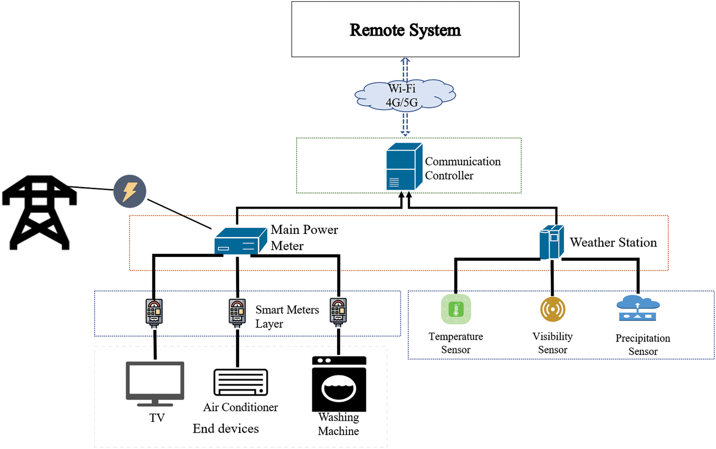
Figure 1: The illustrative diagram of the platform

3.2 Time-Series Analysis

This section presents a synthetic overview of the analysis and processing of the time-series for forecasting. By definition, a time-series refers to a succession of time-based reading recorded at regular spans. For a set of discrete-samples ,..., , where (with ) is the observation at the time , we may then frame the time-series prediction problem as the task of forecasting the values of ,..., , having the preceding samples ,..., (), to nullify the gap between the estimated value and the groungtruth observation ().

Three essential components need to be introduced regarding the time series:

•   Trend—The increasing or decreasing linear behavior of the series over time. A trend can be rising (upward), falling (downward), or flat (stationary).

•   Seasonality—The repeating patterns or cycles of behavior over time. For example, an escalation of the use of the heater in winter because of the drop in temperature.

•   Residual—The variability in observations that cannot be explained by the model.

Other decomposition criteria can equally be included. A key criterion to validate the applicability of time-series data analysis is stationarity. This implies that the mean, variance, and auto-correlation profiles do not change with respect to the time. When a time-series is not stationary, several processing steps are required prior to the implementation of forecasting approaches.

The interaction between these variables must be evaluated to assess the relevance of the feature. The linear and non-linear methods can be investigated depending on the time-series patterns. We refer to the reader to [38–40] for further introduction to time-series analysis.

3.3 Dataset and Pre-Procession

To validate the solution presented in this paper, we have used the Smart* (pronounced smart star) dataset [41] which offers in addition to the records of the electrical loads the climate data of the experimental area. The Smart* dataset includes UMass Smart* Home Data Set and UMass Smart* Microgrid Data Set, which are all collected by installed sensors. Monitoring data from appliances such as the HVAC circulator, clothes dryer, refrigerator, and water heater are collected at a frequency ranging from 30 to 1 min. Weather information is recorded every hour. The data set contains measurements from 7 households for one to three years between 2014 and 2016. The weather station used in the house provides weather attributes such as precipitation, wind speed, temperature, pressure, humidity, etc. The sample size is about 8760 each year. To balance the two subsets of data, we rescaled the power measurement to match the number of records available in the weather information. The frequency was modified to 1 h by summing the consumption between each hour’s time windows.

3.4 Statistical Analysis and Time-Series Data Preparation

The experiment presented in this paper has two parts. The first part of the experiment is to evaluate the correlation between the attributes of the weather dataset and the electricity consumption of the appliances. For this reason, four common non-linear statistical ranking correlation coefficients namely the Maximal Information Coefficient (MIC), the Total Information Coefficient (TIC), Distance Correlation, and the Spearman’s rank correlation coefficient were computed between the two subsets of data. The result is shown in Fig. 2.

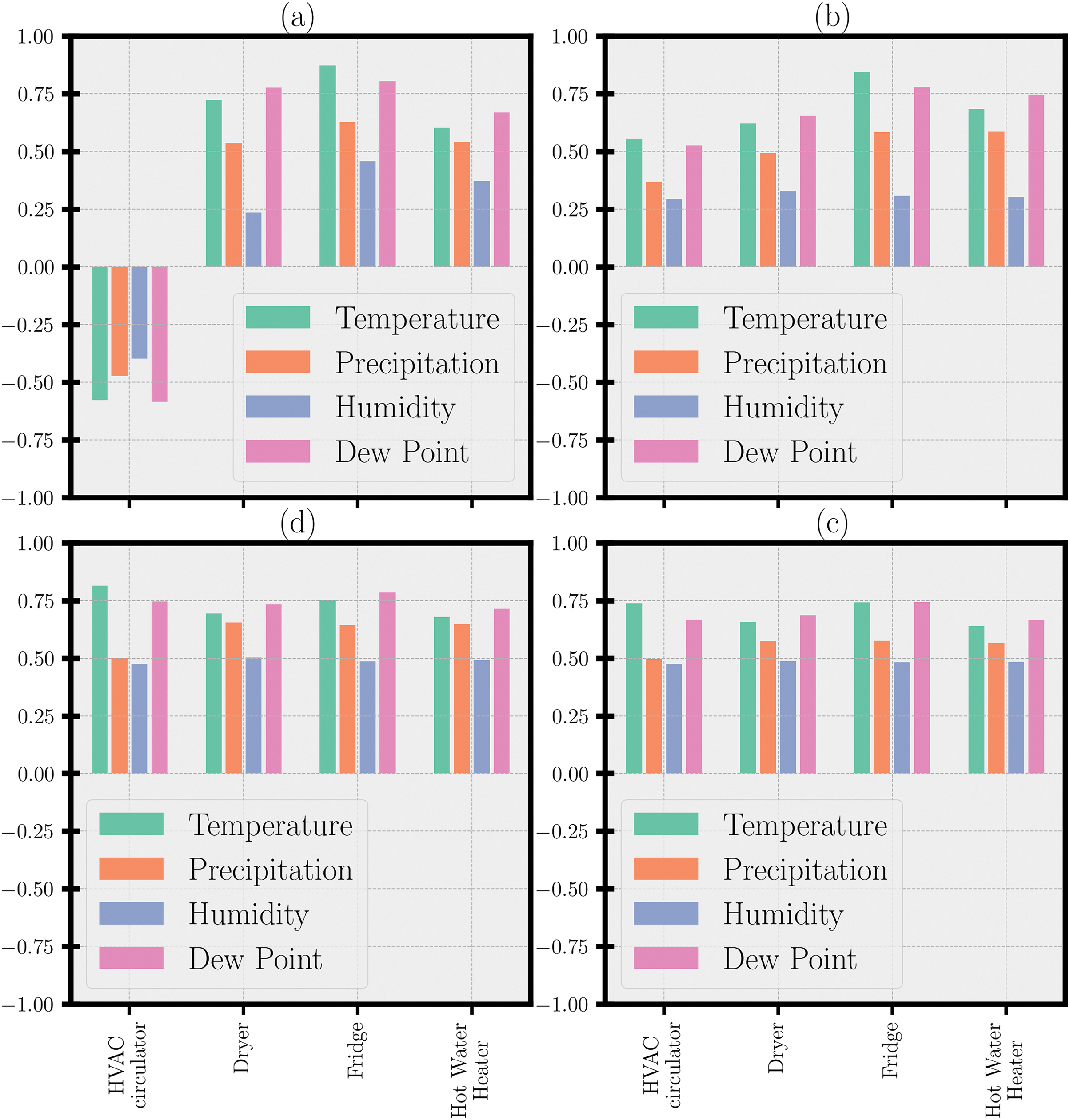
Figure 2: Statistical evaluation of correlation (a) Spearman correlation, (b) Distance correlation, (c) Maximal information coefficient, (d) Total information coefficient

Then a study of the electrical load graph was performed to identify the periodicity of events using the Fast Fourier Transform (FFT). The result can be appreciated in Fig. 3. According to the results, 3 other subsets were created using the most recurrent periods obtained from the FFT evaluation. Based on the frequency domain representation obtained by decomposition, we notice that most devices have their primitives at certain key intervals. The purpose of rescaling is to determine how much energy is consumed during this periodic interval. These are 4, 12, and 24 h. The data was then readjusted under these different frequencies, and the four subsets of data were considered in the continuation of the experiment.

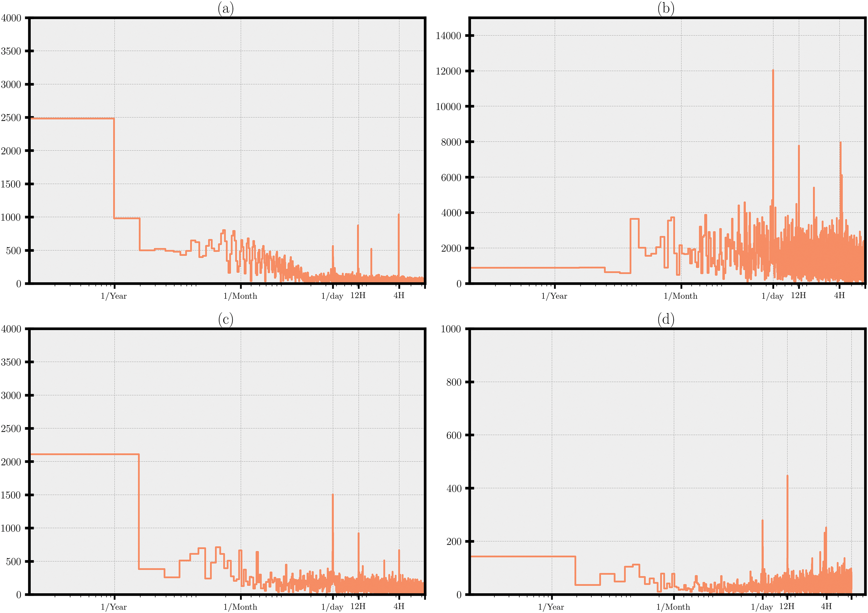
Figure 3: Discrete Fast Fourier transform of the electrical load of appliances (a) HVAC circulator, (b) Dryer, (c) Fridge, (d) Hot Water Heater

To perform the time-series analysis, a major condition is that the data must be stationary. The stationary differentiation and moving average processes with a lag of 5 were applied to the target variables to make them stationary. Then, we calculate the autocorrelation and partial autocorrelation to confirm the effectiveness of the previous process. The result for the HVAC circulator load is shown in Fig. 4.

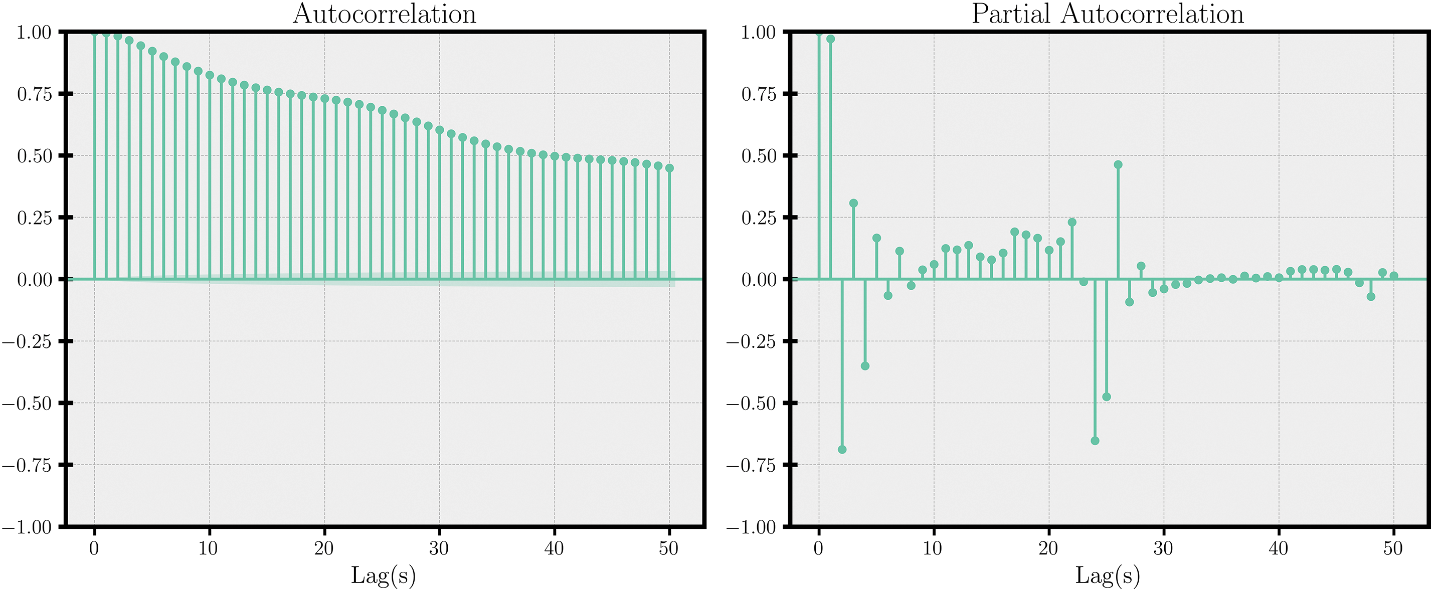
Figure 4: Autocorrelation and partial auto-correlation function on the HVAC circulator load

Feature engineering techniques were used to make raw data suitable for further analysis. The time, day, and month were extracted separately and converted into a periodic sequence using a cosine transform on the time, day, and month in the time-series temporal attribute. Features such as temperature, precipitation, or pressure do not span the same scale. Therefore, preprocessing is required to reduce them to a fixed, standard interval, as machine learning algorithms work best with uniform numerical values. For this reason, the standard scaler was used to transform the entire input axis. The transformation is done according to Eq. (1) where and represent the mean and standard deviation of the input value, respectively, and is the initial value.

(1)

The final step in data processing is data windowing. As mentioned earlier in Section 3.2, the model presented in this paper makes predictions based on a window of consecutive historical observations. The important parameters that drive our analysis are:

•   The size of the historical record is required as input to the algorithm.

•   The prediction horizon represents the distance into the future that the model must predict at one time.

The data must then be formatted into a vector to matrix format for the learning model. The structure is described below. Let be the input at time of feature , the dependent variable at time , the historical horizon, and the prediction horizon. The best performance during the experimental phase was obtained with an input width and prediction horizon set to 24 and 6 observations, respectively. An illustrative Fig. 5 is presented below:

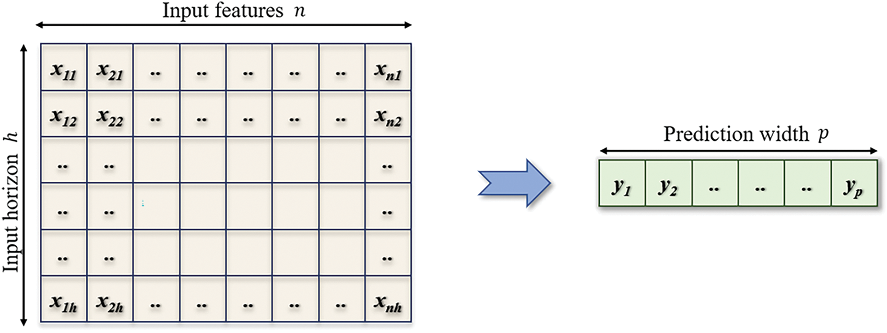
Figure 5: Data windowing format

3.5 Multi Attributes Convolutional Long Short-Term Memory Model

This section presents the sophisticated deep learning model implemented for appliance load prediction. Our base model is a fully connected neural network (FCNN). The model is built by stacking a series of dense layers followed by max-pooling layers and batch normalization layers. The last fully connected layer of our model uses a rectified linear unit as the activation function. The output is then transformed to zero if a negative value is emitted from the previous layers, but for a value greater than zero, no change is made. We also use L2 regularization on the hidden layer for a smoother training phase.

As is shown in Fig. 6.

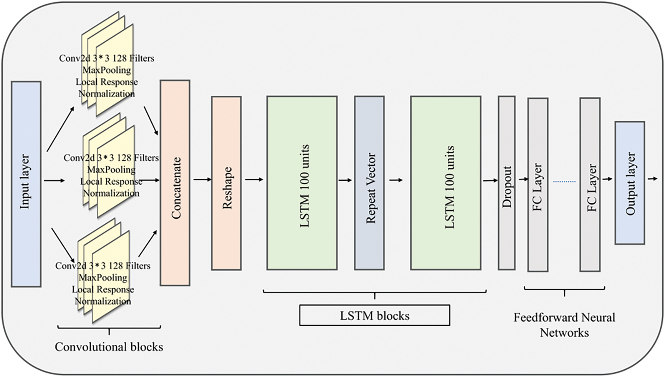
Figure 6: MACLSTM model architecture

This model predicts consumption over a fixed time (relatively short) period in the future. A deep auto-regressive model is derived from this architecture to make long-term forecasting. Using an iterative process, the output of the model at time is reused to produce the prediction at time . This allows for making a medium- and long-term prediction of consumption.

Based on the results of the basic model and various other models, such as convolutional neural network (CNN), long-short term memory (LSTM), bi-directional LSTM (bi-LSTM), Gated Recurrent Units (GRU), and Recurrent Neural Network (RNN), explored in the experimental setting, we designed the proposed Multi Attributes Convolutional Long Short-term Memory (MACLSTM) model in three parts, including convolutional blocks, long short-term blocks and feedforward neural networks.

3.5.1 Convolutional Blocks

The first part of the model uses an improved convolutional architecture for pattern extraction. This model is built using 3 parallel blocks of convolutional layers followed by max-pooling layers [42] and local response normalization (LRN) layers [43]. The convolutional layers use 128 filters and a kernel of size 3 * 3. Convolutional blocks are employed at the beginning of our model to automatically detect the importance of each input feature and the patterns that can be extracted from all input features at once. Local response normalization (LRN) was introduced to improve the generalization ability of CNN blocks and encourage lateral inhibition. We assume that this enables the algorithm to narrow its focus to spatial locations and perform local contrast enhancement so that local maximum values are used as excitation for subsequent layers. The data transfer in the convolutional blocks designed in this paper is depicted in the Fig. 7.

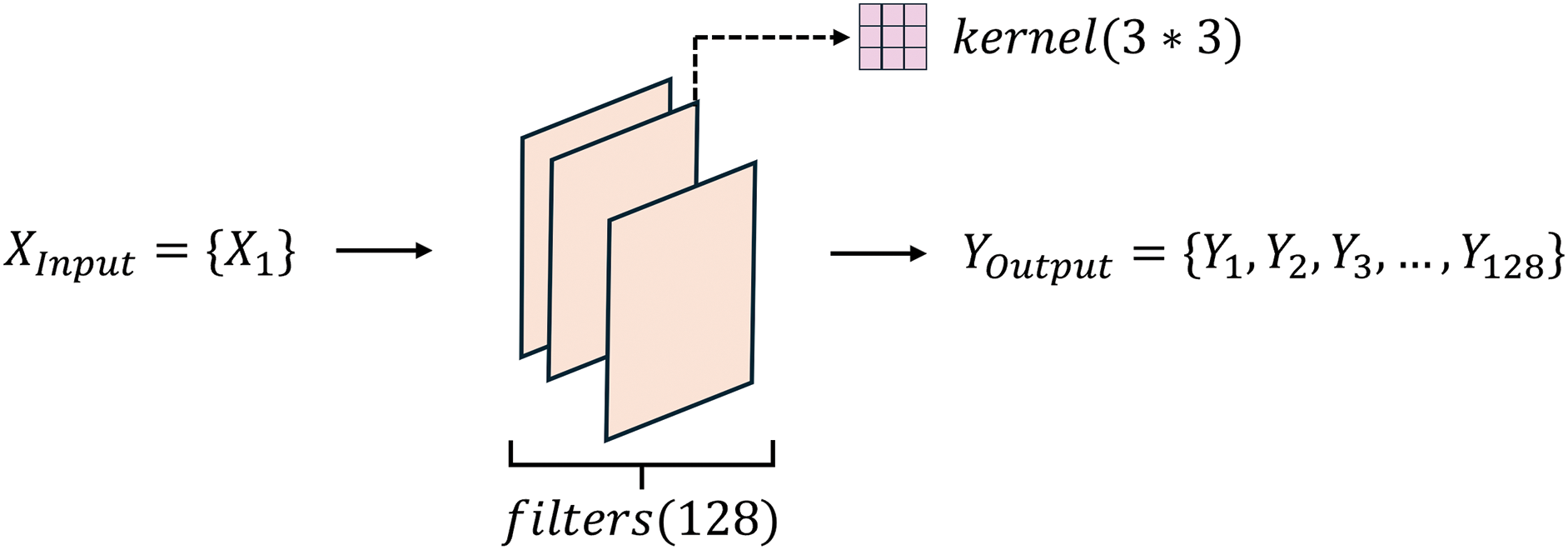
Figure 7: Proposed convolutional blocks architecture

Here, denotes the input sequence, filters (128) indicate the number of kernels in the convolutional layer, kernel (3 * 3) signifies the kernel shape, and denotes the output sequence.

3.5.2 Long Short-Term Memory Blocks

The output of the convolutional blocks is concatenated and reshaped into a 4-dimensional tensor. This tensor is then fed into 100-unit LSTM blocks. A dropout at 0.2 is used at the output of the LSTM block to avoid overfitting. The load inference problem is modeled here as a temporal sequence where connections between consecutive measurements are established. The data transfer process in the LSTM blocks designed in this paper is illustrated in the Fig. 8.

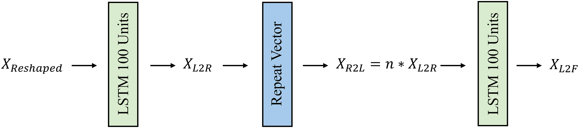
Figure 8: Proposed long short-term memory blocks architecture

Here, signifies the processed data initially extracted from the CNN layer. refers to the data passed from the first LSTM layer to the repeat vector, refers to the data derived after n repetitions by the repeat vector, and refers to the data that continues to propagate forward from the second LSTM layer.

3.5.3 Feedforward Neural Networks

The output tensor is rooted through 4 fully connected layers that have 100, 50, 20, and 1 units, respectively. The rectified linear unit is used throughout the network as the activation function to eliminate any negative values. The model is compiled using the Adam optimizer and the mean square error as the loss function. The data transfer process in the Feedforward networks designed in this paper is shown in the formula below:

(2)

Here, denotes the output data, represents the activation function, denotes the weights, denotes the input data, and denotes the bias.

Define , , , and , and the transfer process of the feedforward network in this paper can be expressed through the following matrix computation.

(3)

4  Experiment Results and Performance

In this section, we present the experimental environment, and the results obtained from various experimental contexts. The experiment was conducted using Python 3.7 and TensorFlow v2.

4.1 Comparative Experiments

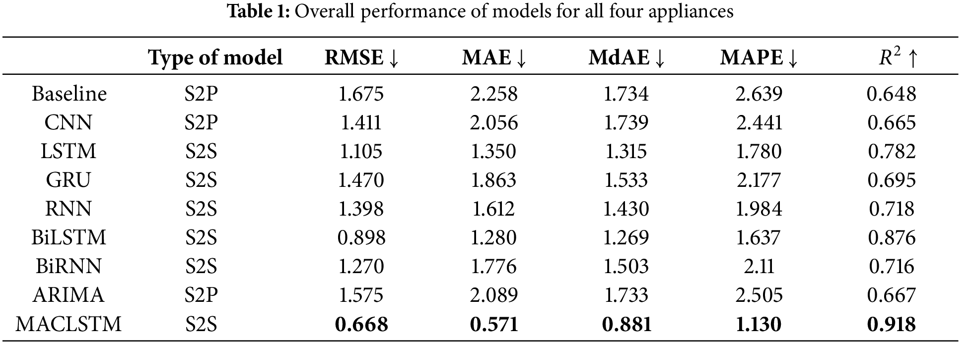
Four appliances from Houses A, G, and H of the Smart* dataset was used for validation. The data is split into 3 subsets named training set, development set, and testing set with respectively 0.8, 0.1, and 0.1 percent of the data. We introduced the preprocessed data in the models designed for this purpose. The batch size was set to 128 and the shuffle was set to False since the relation between consecutive values is important in time-series analysis. An early stop with a patience of 5 was implemented to avoid overtraining the model. The maximum epoch was set to 300 epochs. During the training process, we used a time-based learning rate decay to reduce the learning rate until local minima is obtained. Several common prediction metrics are used to evaluate the model: the Root Mean Squared Error (RMSE) in Eq. (2), the Mean Absolute Error (MAE) in Eq. (3), the Median Absolute Error (MdAE) in Eq. (4), the Mean Absolute Percentage Error (MAPE) in Eq. (5), and the Coefficient of determination (R2) in Eq. (6) defines how well the changes in the input data is reflected in the models’ output. The average training results for all models at various frequencies are presented in Table 1 where two types of model architectures were evaluated: the sequence-to-sequence (S2S) models and the sequence-to-point (S2P) models. In Table 1, “” represents that the larger the value is, the better the performance will be. The bold value represents that the model achieves the best performance.

(4)

(5)

(6)

(7)

(8)

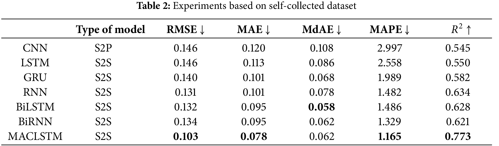
A self-collected dataset was also used. The dataset included load data from 10 rooms in a building from 01 September 2020 to 01 September 2022, collected with a frequency of once a day. The parameter settings of the model remained the same. As shown in Table 2, MACLSTM achieved the best performance in terms of RMSE, MAE, MAPE and . Among them, increased by 21.9%, compared to RNN model.

4.2 Ablation Experiments

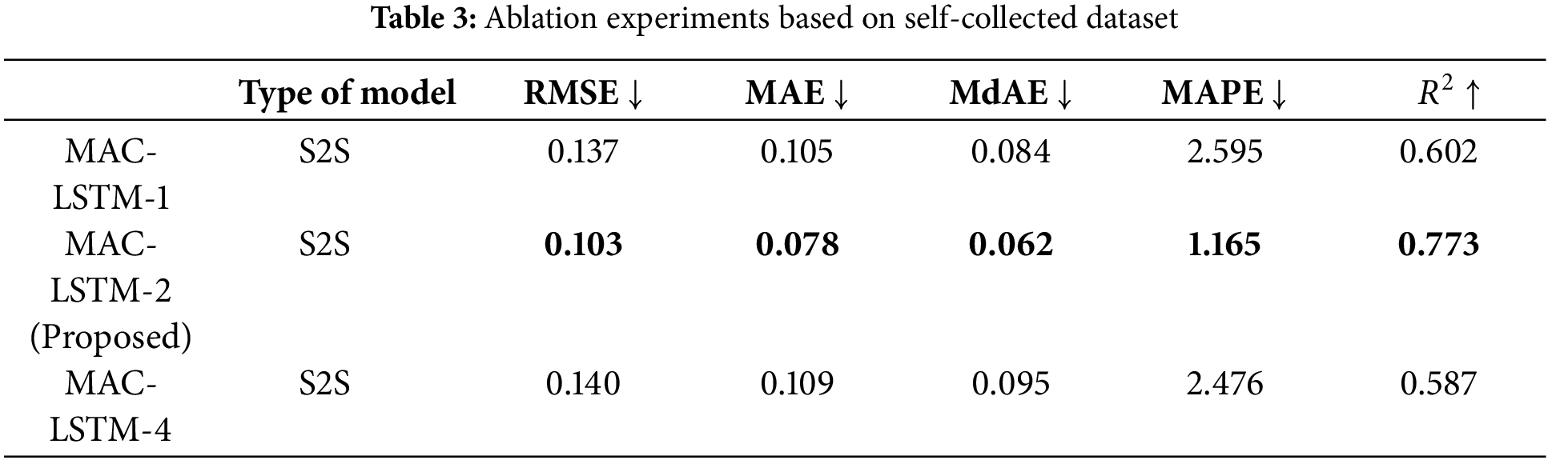
The ablation experiments were used to set the number of LSTM layers. The number of layers in the model needs to be limited to prevent overfitting, so the number is set to 1, 2, and 4. MAC-LSTM-1 represent that the model consisted of 1 LSTM layer. As shown in Table 3, MAC-LSTM-2 achieved the best performance, so we set the number of LSTM layers to 2.

5  Discussion

In this study, we present an innovative method to predict the consumption of household appliances. The experiments were conducted on redefined data into four different frequencies and the deduction of the waveforms that constitute the load of each appliance. In general, the most successful results were achieved when the frequency was in the range of 1 to 4 h for most of the devices. This could be explained by the fact that these durations are consequent enough to contain a complete cycle of all the operating modes of the device. When the experiments are performed on the daily data, the performance decreased the most because this transformation not only concealed several patterns that occurred during the day but also considerably reduced the amount of information fed to the model. The model proposed in this paper outperforms commonly used approaches. We hypothesize that this could be explained by the increased ability to generalize offered by the improved CNN blocks used to detect modalities in the data. A comparison using RMSE and R-squared of the models is presented in Fig. 9. A loss of performance is however observed for some appliances such as the Dryer, and it may be caused by the periodic use of the devices. Indeed, the operating mode of these appliances would not be strongly linked to climate factors. Nevertheless, the existing relations between the successive observations made it possible to detect most of the sequences of the utilization of these devices.

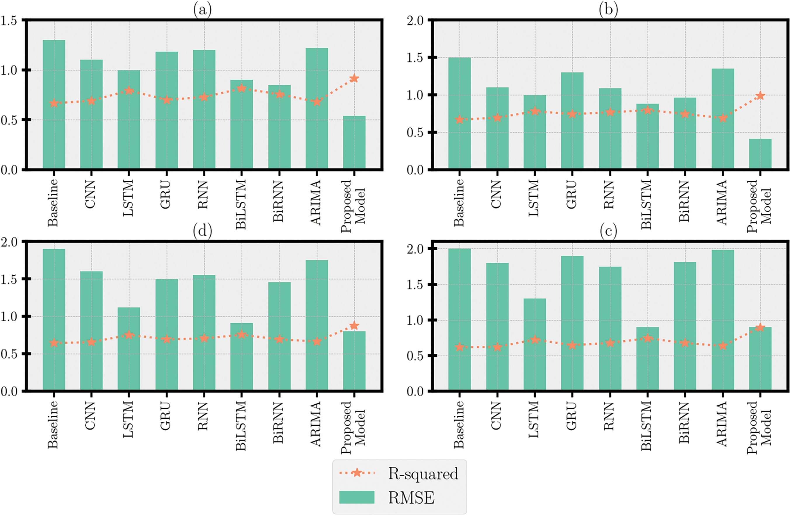
Figure 9: Comparison of the RMSE and obtained by all models for each subset of data. The sampling frequencies were (a) 1 h, (b) 4 h, (c) 12 h, (d) 24 h

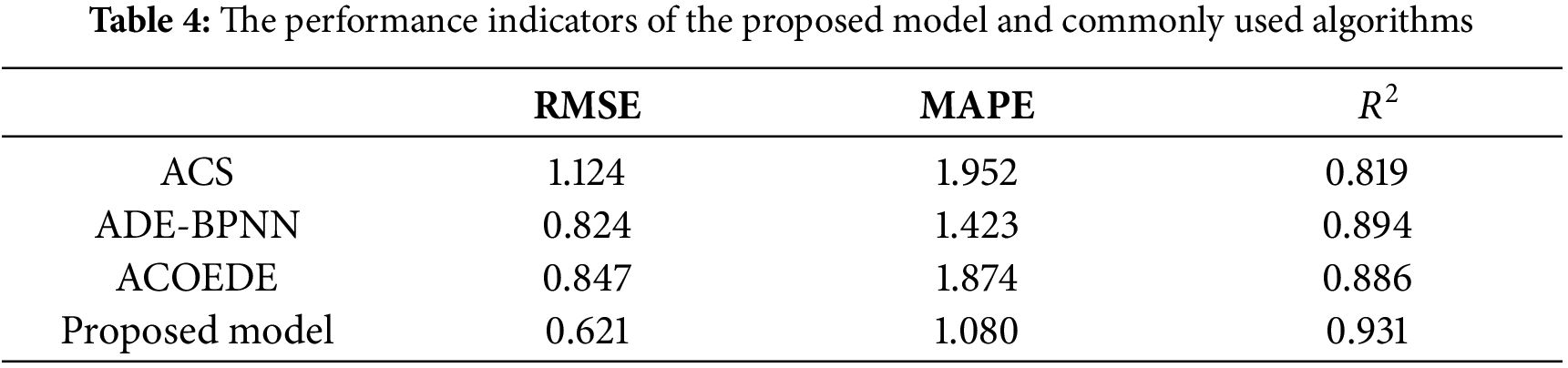
The scores of the proposed model were benchmarked against the performance of the Artificial Cooperative Search (ACS) [44], Adaptive Differential Evolution-back-propagation neural network (ADE–BPNN) [45], and the ant colony optimization energy demand estimation (ACOEDE). During this process, the entire data set was used to carry out performance testing of the model. Table 4 summarized the performance indicators based on RMSE, MAPE, and R2.

Although the experiments focused more on short-term forecasting, the solution proposed in this work is also suitable for medium and long-term forecasting when the historical data frequency is properly formatted. This could be the subject of future investigation.

6  Summary and Future Work

This study focused on the proposal of an ingenious method for electric energy prediction using climate data. The paper presents a statistical study to establish the degree of relationship between climate variables and the electrical consumption of appliances. A decomposition of the graph obtained from the monitored electrical load was then carried out. A deep learning model was subsequently implemented and evaluated on data from real households. The experimental results showed that the proposed method offers better performance than the state-of-the-art models in most cases. Since not all devices have the same internal structure, some devices seem not to respond favorably to the proposed solution. Compared to current popular models, MACLSTM did not achieve the best performance on all indicators in the experiments based on self-collected datasets, but its prediction accuracy was more stable. In addition, the performances of our proposed MACLSTM are different based on the two data sets. Therefore, the generalization of the model needs further testing, and we will test our model on more data sets. The future research can be directed towards the development of a collaborative method that will combine the strengths of several existing solutions.

Acknowledgment: All authors would like to express thanks to the editors.

Funding Statement: This research was funded by NARI Group’s Independent Project of China (Grant No. 524609230125) and the Foundation of NARI-TECH Nanjing Control System Ltd. of China (Grant No. 0914202403120020).

Author Contributions: The authors confirm contribution to the paper as follows: study conception and design: Ruoxin Li, Shaoxiong Wu; data collection: Fengping Deng, Hua Cai; analysis and interpretation of results: Zhongli Tian, Xiang Li, Xu Xu; draft manuscript preparation: Qi Liu, Fengping Deng. All authors reviewed the results and approved the final version of the manuscript.

Availability of Data and Materials: The data that support the findings of this study are openly available in Smart* in reference [41].

Ethics Approval: Not applicable.

Conflicts of Interest: The authors declare no conflicts of interest to report regarding the present study.

References

1. Abdulla N, Demirci M, Ozdemir S. Smart meter-based energy consumption forecasting for smart cities using adaptive federated learning. Sustainable Energy Grids Netw. 2024;38:101342. doi:10.1016/j.segan.2024.101342. [Google Scholar] [CrossRef]

2. Bowa KC, Mwanza M, Sumbwanyambe M, Ulgen K, Pretorius JH. Comparative sustainability assessment of electricity industries in SADC region: the role of renewable energy in regional and national energy diversification. In: 2019 IEEE 2nd International Conference on Renewable Energy and Power Engineering (REPE); 2019; Toronto, ON, Canada. p. 260–8. [Google Scholar]

3. Stratman A, Hong T, Yi M, Zhao D. Net load forecasting with disaggregated behind-the-meter PV generation. IEEE Trans Ind Appl. 2023;59(5):5341–51. doi:10.1109/TIA.2023.3276356. [Google Scholar] [CrossRef]

4. Luo Z, Peng J, Tan Y, Yin R, Zou B, Hu M, et al. A novel forecast-based operation strategy for residential PV-battery-flexible loads systems considering the flexibility of battery and loads. Energy Convers Manage. 2023;278:116705. doi:10.1016/j.enconman.2023.116705. [Google Scholar] [CrossRef]

5. Liu Y, Zhang D, Gooi HB. Optimization strategy based on deep reinforcement learning for home energy management. CSEE J Power Energy Syst. 2020;6(3):572–82. [Google Scholar]

6. Biswal B, Deb S, Datta S, Ustun TS, Cali U. Review on smart grid load forecasting for smart energy management using machine learning and deep learning techniques. Energy Rep. 2024;12:3654–70. doi:10.1016/j.egyr.2024.09.056. [Google Scholar] [CrossRef]

7. Ali S, Bogarra S, Riaz MN, Phyo P, Flynn D, Taha A. From time-series to hybrid models: advancements in short-term load forecasting embracing smart grid paradigm. Appl Sci. 2024;14(11):4442. doi:10.3390/app14114442. [Google Scholar] [CrossRef]

8. Hnin SW, Karnjana J, Kohda Y, Jeenanunta C. A hybrid K-means and KNN approach for enhanced short-term load forecasting incorporating holiday effects. Energy Rep. 2024;12:5942–59. doi:10.1016/j.egyr.2024.11.050. [Google Scholar] [CrossRef]

9. Han L, Wang X, Yu Y, Wang D. Power load forecast based on CS-LSTM neural network. Mathematics. 2024;12(9):1402. doi:10.3390/math12091402. [Google Scholar] [CrossRef]

10. Fan J, Zhuang W, Xia M, Fang W, Liu J. Optimizing attention in a transformer for multihorizon, multienergy load forecasting in integrated energy systems. IEEE Trans Ind Inform. 2024;20(8):10238–48. doi:10.1109/TII.2024.3392278. [Google Scholar] [CrossRef]

11. Chujai P, Kerdprasop N, Kerdprasop K. Time series analysis of household electric consumption with ARIMA and ARMA models. Proc Int Multiconf Eng Comput Sci. 2013;1:295–300. [Google Scholar]

12. Han D, Bai H, Wang Y, Bu F, Zhang J. Day-ahead aggregated load forecasting based on household smart meter data. Energy Rep. 2023;9(8):149–58. doi:10.1016/j.egyr.2023.04.317. [Google Scholar] [CrossRef]

13. Moreno Jaramillo AF, Laverty DM, Morrow DJ, del Rincon MJ, Foley AM. Load modelling and non-intrusive load monitoring to integrate distributed energy resources in low and medium voltage networks. Renew Energy. 2021;179:445–66. doi:10.1016/j.renene.2021.07.056. [Google Scholar] [CrossRef]

14. Chen T, Wan W, Li X, Qin H, Yan W. Flexible load multi-step forecasting method based on non-intrusive load decomposition. Electronics. 2023;12(13):2842. doi:10.3390/electronics12132842. [Google Scholar] [CrossRef]

15. Kaneko N, Okazawa K, Zhao D, Nishikawa H, Taniguchi I, Murayama H, et al. Non-intrusive thermal load disaggregation and forecasting for effective HVAC systems. Appl Energy. 2024;367:123379. doi:10.1016/j.apenergy.2024.123379. [Google Scholar] [CrossRef]

16. Mengistu MA, Girmay AA, Camarda C, Acquaviva A, Patti E. A cloud-based on-line disaggregation algorithm for home appliance loads. IEEE Trans Smart Grid. 2018;10(3):3430–9. doi:10.1109/TSG.2018.2826844. [Google Scholar] [CrossRef]

17. Cha SC, Chuang MS, Yeh KH, Huang ZJ, Su C. A user-friendly privacy framework for users to achieve consents with nearby BLE devices. IEEE Access. 2018;6:20779–87. [Google Scholar]

18. Ruano A, Hernandez A, Ureña J, Ruano M, Garcia J. NILM techniques for intelligent home energy management and ambient assisted living: a review. Energies. 2019;12(11):2203. [Google Scholar]

19. Marah BD, Jing Z, Ma T, Alsabri R, Anaadumba R, Al-Dhelaan A, et al. Smartphone architecture for edge-centric IoT analytics. Sensors. 2020;20(3):892. [Google Scholar] [PubMed]

20. Liu Y, Peng M, Shou G, Chen Y, Chen S. Toward edge intelligence: multiaccess edge computing for 5G and Internet of Things. IEEE Internet Things J. 2020;7(8):6722–47. [Google Scholar]

21. Brody P, Pureswaran V. Device democracy: saving the future of the internet of things—IBM global business services executive report. IBM Glob Bus Serv Exec Rep. 2015:3–25. [Google Scholar]

22. Ma W, Wei X, Wang L. A security-oriented data-sharing scheme based on blockchain. Appl Sci. 2024;14(16):6940. [Google Scholar]

23. Chen Z, Cai L. User-preference-aware private-preserving average consensus. In: 2019 IEEE Pacific Rim Conference on Communications, Computers and Signal Processing (PACRIM); 2019; Victoria, BC, Canada; IEEE. p. 1–6. [Google Scholar]

24. Shen J, Zhou T, He D, Zhang Y, Sun X, Xiang Y. Block design-based key agreement for group data sharing in cloud computing. IEEE Trans Dependable Secure Comput. 2017;16(6):996–1010. [Google Scholar]

25. Xu X, Fang Z, Qi L, Zhang X, He Q, Zhou X. TripRes: traffic flow prediction driven resource reservation for multimedia IoV with edge computing. ACM Trans Multimed Comput Commun Appl. 2021;17(2):41. [Google Scholar]

26. Li X, Wang Q, Lan X, Chen X, Zhang N, Chen D. Enhancing cloud-based IoT security through trustworthy cloud service: an integration of security and reputation approach. IEEE Access. 2019;7:9368–83. [Google Scholar]

27. Wei X, Wang S, Zhou A, Xu J, Su S, Kumar S, et al. MVR: an architecture for computation offloading in mobile edge computing. In: 2017 IEEE International Conference on Edge Computing (EDGE); 2017; Honolulu, HI, USA. p. 232–5. [Google Scholar]

28. Osathanunkul K, Osathanunkul K. Different sampling rates on neural NILM energy disaggregation. In: 2019 Joint International Conference on Digital Arts, Media and Technology with ECTI Northern Section Conference on Electrical, Electronics, Computer and Telecommunications Engineering (ECTI DAMT-NCON); 2019; Nan, Thailand: IEEE. p. 318–21. doi:10.1109/ECTI-NCON.2019.8692281. [Google Scholar] [CrossRef]

29. Kaselimi M, Doulamis N, Voulodimos A, Protopapadakis E, Doulamis A. Context aware energy disaggregation using adaptive bidirectional LSTM models. IEEE Trans Smart Grid. 2020;11(4):3054–67. [Google Scholar]

30. Makonin S, Ellert B, Bajić IV, Popowich F. Electricity, water, and natural gas consumption of a residential house in Canada from 2012 to 2014. Sci Data. 2016;3:160037. [Google Scholar] [PubMed]

31. Kane T, Firth SK, Hassan TM, Dimitriou V. Heating behaviour in English homes: an assessment of indirect calculation methods. Energy Build. 2017;148:89–105. [Google Scholar]

32. Johnson MJ, Kolter JZ. REDD: A public data set for energy disaggregation research. In: Workshop on Data Mining Applications in Sustainability (SIGKDD); 2011; San Diego, CA, USA. [Google Scholar]

33. Hart GW. Nonintrusive appliance load monitoring. Proc IEEE. 1992;80(12):1870–91. [Google Scholar]

34. Komatsu H, Kimura O. A combination of SOM-based operating time estimation and simplified disaggregation for SME buildings using hourly energy consumption data. Energy Build. 2019;201:118–33. [Google Scholar]

35. Pipattanasomporn M, Chitalia G, Songsiri J, Aswakul C, Pora W, Suwankawin S, et al. CU-BEMS, smart building electricity consumption and indoor environmental sensor datasets. Sci Data. 2020;7(1):241. [Google Scholar] [PubMed]

36. Lee TK, Kim JU. A cost-effective and heuristic approach for building energy consumption prediction: BES model calibration and forecasting algorithm. Energy Build. 2024;303:113800. [Google Scholar]

37. Faiq M, Geok Tan K, Pao Liew C, Hossain F, Tso CP, Li Lim L, et al. Prediction of energy consumption in campus buildings using long short-term memory. Alex Eng J. 2023;67:65–76. [Google Scholar]

38. Martins A, Lagarto J, Canacsinh H, Reis F, Cardoso MGMS. Short-term load forecasting using time series clustering. Optim Eng. 2022;23(4):2293–314. [Google Scholar]

39. Gan J, Zeng L, Liu Q, Liu X. A survey of intelligent load monitoring in IoT-enabled distributed smart grids. Int J Ad Hoc Ubiquitous Comput. 2023;42(1):12–29. doi:10.1504/ijahuc.2023.127781. [Google Scholar] [CrossRef]

40. Dab K, Henao N, Nagarsheth S, Dubé Y, Sansregret S, Agbossou K. Consensus-based time-series clustering approach to short-term load forecasting for residential electricity demand. Energy Build. 2023;299:113550. doi:10.1016/j.enbuild.2023.113550. [Google Scholar] [CrossRef]

41. Barker S, Mishra A, Irwin D, Cecchet E, Albrecht J. Smart*: an open data set and tools for enabling research in sustainable homes. In: ACM SustKDD’12; 2012; Beijing, China. [Google Scholar]

42. Jaśkowski M, Świątkowski J, Zając M, Klimek M, Potiuk J, Rybicki P, et al. Improved GQ-CNN: deep learning model for planning robust grasps. arXiv:1802.05992. 2018. [Google Scholar]

43. Krizhevsky A, Sutskever I, Hinton GE. ImageNet classification with deep convolutional neural networks. Commun ACM. 2017;60(6):84–90. doi:10.1145/3065386. [Google Scholar] [CrossRef]

44. Kaboli SHA, Selvaraj J, Rahim NA. Long-term electric energy consumption forecasting via artificial cooperative search algorithm. Energy. 2016;115:857–71. doi:10.1016/j.energy.2016.09.015. [Google Scholar] [CrossRef]

45. Zeng YR, Zeng Y, Choi B, Wang L. Multifactor-influenced energy consumption forecasting using enhanced back-propagation neural network. Energy. 2017;127:381–96. doi:10.1016/j.energy.2017.03.094. [Google Scholar] [CrossRef]