Two-Phase Software Fault Localization Based on Relational Graph Convolutional Neural Networks

1  Introduction

With the increasing size and complexity of software, unexpected faults may occur due to programming errors or immature development processes. Developers need to invest a lot of time and resources to debug the software, find out the specific location of the faults and solve them. According to statistics, the cost of debugging software faults may account for 80% of the total cost of software [1]. In the debugging process, fault localization is extremely expensive and time-consuming. Therefore, high-precision and efficient fault localization techniques are needed to simplify the debugging process.

In recent decades, researchers have proposed a variety of automated fault localization techniques, among which spectrum-based fault localization (SBFL) has become one of the most widely studied techniques due to its effectiveness and lightweight. However, SBFL has a significant issue where all statements within a basic block have the same suspicion value, making it impossible to locate the faulty statement more precisely in the program. Previous studies addressed this issue by generating a large number of mutated programs, also known as mutation-based fault localization (MBFL) [2]. With the rapid development of machine learning and deep learning, many researchers have adopted neural network-based methods to mine the potential features of code elements [3], aiming to achieve precise localization.

Graph neural network (GNN) is a kind of deep learning model designed to process graph data. Different from traditional neural networks that can only handle euclidean space data, GNNs can deal with graph data in non-euclidean space. In recent years, GNNs-based fault localization techniques have achieved promising results. These methods employ intermediate data representations such as abstract syntax trees (ASTs) [4], control flow graphs (CFGs) [5], or program dependence graphs (PDGs) [6] to abstract source code into graph structures. However, these graph representations do not include inter-class dependencies, and research has shown that over 20% of faults belong to inter-class method call type [7]. In addition, in widely used fault localization datasets (e.g., Defects4J), projects code can span tens of thousands of lines. Directly constructing graph representations of such extensive source code would result in an overly large graph, leading to a waste of computational resources and increasing the training burden of GNNs.

This paper proposes a novel two-phase software fault localization based on relational graph convolutional neural networks (Two-RGCNFL). This method aims to address the issue of parallel ranking of suspicious elements in traditional SBFL technology. Additionally, this work also comprehensively considers the data and control dependencies within and between classes, which can locate more inter-class method call type faults. Specifically, in Phase 1, this work constructs a method call dependency graph (MCDG) with methods as nodes and control dependencies and data dependencies as edges. This graph is cross-class, thereby containing rich intra-class and inter-class dependencies. Then relational graph convolutional neural network (RGCN) is employed to extract node features from the MCDG and utilize a classifier to identify faulty methods. Since MCDG is a multi-relational graph with extremely unbalanced classes, we also improve the GraphSMOTE algorithm to mitigate the impact of class imbalance on classification accuracy. Finally, in Phase 2, this work constructs a RankNet model with shared weight siamese multi-layer perceptron (MLP) as the main frame structure. With the ability of MLP to capture subtle differences in node features, we can effectively distinguish suspicious values of statements in the same basic block. The main contributions of this paper are as follows:

1.    In view of the fact that previous researchers only considered intra-class dependencies when abstractive the source code as a graph structure, this paper proposes MCDG. MCDG is simplified from system dependence graph (SDG), which can not only reduce the training burden of GNN, but also contain rich intra-class and inter-class method call dependencies, so that GNN can mine more abundant node feature information.

2.    Aiming at the problem that GraphSMOTE algorithm can only deal with a single relational graph structure, this paper improves it to solve the class imbalance problem of multi-relational graphs.

3.    Two-RGCNFL is proposed, which can achieve more accurate localization by gradually narrowing the localization range in a phased manner. In addition, Two-RGCNFL can effectively solve the problem of parallel ranking of suspicious elements in traditional SBFL technology.

4.    This paper conducted experiments on 5 projects in the Defects4J benchmark and evaluated the experimental results using two evaluation metrics: Top-K and mean reciprocal rank. The results indicate that Two-RGCNFL can achieve better performance compared with all the baseline methods in this paper.

The remaining organization of this paper is as follows: Section 2 reviews the related research on fault localization and introduces the tools used in this paper. Section 3 details the methodological framework of this paper. Section 4 introduces the main research questions, experimental datasets, evaluation metrics and parameter setting. Section 5 analyzes the experimental results in detail. Section 6 discusses statistical significance test and potential threats to validity. Section 7 provides a brief summary of the paper and future perspectives.

2  Related Work

2.1 Spectrum-Based Fault Localization

SBFL is a typical method in dynamic analysis. The input of SBFL is the code coverage information of all test cases, while its output is a descending list of suspicious values calculated by code elements according to their specific formulas. The “spectrum” in SBFL refers to the set of runtime code coverage information, which is a description form of dynamic behavior characteristics of program runtime [8].

SBFL has become one of the most widely studied techniques due to its ease of obtaining program spectra and its intuitive reflection of program runtime information. Zhang et al. [9] proposed to use PageRank algorithm to analyze the relationship between test cases and the program under test, thereby taking into account the contributions of different test cases and recalculating the spectra. The traditional SBFL technique was then applied to the recalculated spectra. Experiments showed that the performance of this method was significantly better than the state-of-the-art SBFL techniques. By introducing the local influence calculation of software entities, Zhao et al. [10] proposed a spectrum-enhanced fault localization method, which could make full use of the internal interaction information between software entities. They also proposed a new suspicion measure, namely fault centrality, which is used to comprehensively evaluate the suspicion level of methods. Widyasari et al. [11] took into account two facts. The first is that not all failing test cases contribute equally to the fault under consideration. The second is that program units cooperate in different ways causing test cases to fail. So, they propose to use interpretable artificial intelligence (AI) techniques to learn the local relationship between program units and the fail/pass outcome of each test case. The unique contribution of failed test cases to the suspiciousness of a program unit is automatically learned by learning the different and collaborative contributions of a program unit to the execution outcome of each test case. However, the statistical formulas relied upon by SBFL techniques do not always yield satisfactory results in multi-fault programs, so Callaghan et al. [12] proposed fault localization by iterative test suite reduction (FLITSR). For programs with multiple faults, the location of fault elements is influenced by the density of failed tests executing each fault. To accurately locate faults one by one from a multi-fault program, FLITSR can increase the relative density of failed tests executing the remaining faulty elements by removing the failed tests executing the most suspicious elements from the test suite, thus improving the ranking of these faults. Although many SBFL techniques proposed by researchers demonstrate good performance to some extent, modern software programs are increasingly complex and large-scale, making it difficult to accurately locate faults solely through spectra and statistical formulas. On this basis, we also delve into the fault propagation contexts and potential features of code elements.

2.2 Deep Learning-Based Fault Localization

Fault localization methods based on deep learning can extract and mine the potential features of code elements, accomplishing the localization task through feature learning. Li et al. [13] utilized the image classification and pattern recognition capabilities of convolutional neural networks (CNN) to achieve localization through code coverage representation learning and data dependence of program statements. Cao et al. [14] proposed DeepFD, a learning-based fault diagnosis and localization framework, which maps the fault localization task to a learning problem. Specifically, DeepFD diagnoses and locates faults in deep learning programs by inferring suspicious fault types using features extracted during model training, and then locates the faults diagnosed in deep learning programs. Zhang et al. [15] used test cases to train CNN, leveraging weight-sharing of CNN to significantly reduce the number of parameters in the model. However, this method requires high-quality test cases. Yang et al. [16] proposed a fault localization method that does not require running any test cases. They utilize the representations learned from pre-trained language models, which already contain abundant knowledge about statement suspicious, to identify faults. Meng et al. [17] proposed TRANSFER, which exploits deep semantic features and knowledge transferred from open-source data to improve fault localization and program repair. Firstly, two large-scale error datasets are constructed to learn the deep semantic features of sentences, respectively. The semantic-based, mutation-based and mutation-based features are then combined and the MLP-based model is used for fault localization. In addition, GNNs have demonstrated powerful graph structural learning capabilities in recent years. Lou et al. [18] proposed a new graph representation of programs that uses gated graph neural networks to learn useful features from the graph and rank program entities. Qian et al. [4] used graph convolutional neural network to collect the static and dynamic features of nodes from the AST and coverage information. They then used GraphSAGE to obtain the node representations of the source code, and finally applied an MLP to output the suspicious values of program entities. Gou et al. [19] proposed a fault location method based on network spectrum that combined test data and software network. This method analyzes and tests software source code to obtain software network and program spectra, then establishes network spectra and carries out feature dimension reduction and class imbalance processing on it, and finally utilizes GNN model to construct a multiple fault location model based on network spectra. Rafi et al. [20] integrate inter-procedural method calls and historical code evolution into the graph representations, enhancing code representations with dependency-augmented coverage graphs and providing GNNs with historical code evolution information, achieving superior performance results. Numerous studies have shown that deep learning can also obtain excellent performance in the field of software fault localization, and thus, we also employ deep learning in our research to accomplish fault localization tasks.

2.3 System Dependence Graph

SDG and PDG are intermediate program representations. PDG was first introduced by Mantovani et al. [21] in 1987, which explicitly defines the data dependency and control dependency of each operation within the program. In a PDG, nodes represent statements or predicate expressions, while edges represent dependency relationships. SDG extends the PDG of a single program to effectively analyze the dependency relationships across different classes. In addition to the nodes and edges in the PDG, the SDG contains dependency edges that represent the context of procedure calls. Due to the rich information about source code structure and dependency relationships contained within SDG, they have been widely used in vulnerability detection and program slicing.

Karuthedath et al. [22] proposed a method to generate test cases for Java programs based on SDG to test whether there is an array index boundary overflow in the program. During parsing the input Java source code, a separate node is created for each class, and the control flow graph in SDG is used to generate a path for each method in the source code, and the data dependence graph is used to track the last definition of the array index variable and obtain the expression that causes the change of the index variable value. Wang et al. [23] proposed a subsentence-level dependency graph (SSLDG) based on system dependency graph, which is built from fine-grained dependencies of object-oriented programs. With SSLDG, they also proposed a new slicing algorithm that can exploit fine-grained dependencies to compute accurate slicing results. To our knowledge, most current research on fault localization mainly obtains the intra-class dependencies through PDG, but few researchers consider the dependency relationship between different classes. This relationship contained in SDG can provide important information for fault localization.

3  Approach

This paper proposes Two-RGCNFL, which comprises two phases: the method classification phase and the statement ranking phase. The former considers both intra-class and inter-class method call dependencies, while the latter addresses the limitations of traditional SBFL technology and realizes a finer-grained fault localization. This section will introduce Two-RGCNFL in detail.

The Two-RGCNFL framework is shown in Fig. 1, which is divided into three main steps. (1) Data preparation: Firstly, the project source code is extracted from Defects4J. The traditional SBFL technique is applied to obtain the suspicious values of each method and sort them. The MCDG is constructed and then pruned according to the ranking of suspicious values to narrow down the localization range. The improved GraphSMOTE [24] is used to address the issue of node class imbalance. (2) Method-level classification phase: The RGCN model is trained to predict whether a method is faulty or not. (3) Statement-level ranking phase: For methods that may contain faults, Doc2Vec [25] is utilized to convert each statement within the method into a low-dimensional vector representation. These vectors are concatenated with the statement spectrum information to form the feature vector of the statements. By training the siamese MLP within the RankNet model, the suspicious values of the statements are output and sorted.

Figure 1: The overall framework of Two-RGCNFL

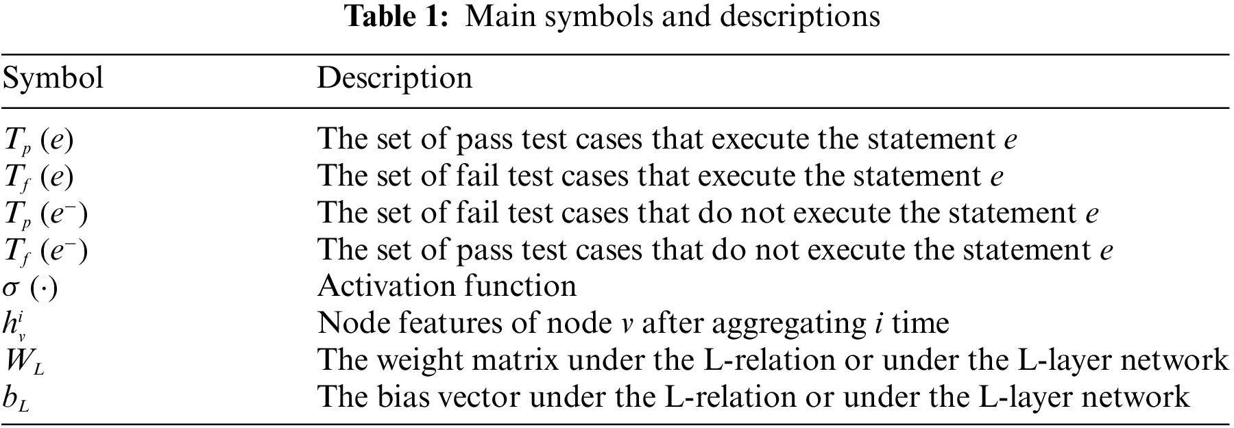
In addition, to facilitate the understanding of the proposed approach, we provide the main formula symbols used in this paper and their descriptions, as shown in Table 1.

3.1 Data Preparation

3.1.1 Program Spectrum

Firstly, we check out the source code of the 5 projects from the Defects4J. For each faulty version, this paper employed SBFL technique to calculate the suspicious value for each method. The cornerstone of SBFL technology lies in program spectra, which can be classified into statement coverage, branch coverage and method coverage. To achieve statement-level localization in Phase 2, this paper adopted the statement coverage spectrum. In this section, statement coverage data is collected by executing test cases, and the execution results of these test cases are recorded simultaneously. The mainstream SBFL technique primarily relies on the following factors to calculate the suspicious value of the statements: , , and . According to the above four values, the suspicious value of each statement is calculated using specific formulas such as Dstar [26], Ochiai [27]. Compared with the three others, Dstar has been proved to have the best and most effective comprehensive ranking performance [28], so we choose Dstar, whose formula is shown in Eq. (1):

(1)

(2)

For a method that contains statements, each of which has a suspicious value. The suspicious value of the method can be expressed by Eq. (2), which is the maximum value of suspicious value of all statements within the method.

3.1.2 Method Call Dependency Graph

An SDG includes a program dependence graph of the system’s main program, the process dependence graph of the system’s auxiliary program and some additional edges. An SDG of a complete software system can be extremely vast, containing numerous irrelevant information that can interfere with the training of GNN. In this section, this paper proposes a new graph representation of programs, namely MCDG. Derived from the simplification of SDG, MCDG utilizes methods as nodes and the dependencies between methods as edges. This graph structure excludes the internal structure information of each method, which can effectively reduce the noise in the graph during the method-level classification phase. Next, we describe the construction of MCDG.

In the original SDG, there are 6 kinds of nodes. In fact, the call node belongs to the control flow node. The actual-in, actual-out, formal-in, and formal-out nodes are used for information transfer and thus fall under the data flow nodes. However, MCDG is constructed at the method granularity, and the internal implementation of method is opaque. So, for most nodes in the graph, the same node may simultaneously belong to actual-in, actual-out, formal-input, and formal-out categories. For ease of understanding, this paper simplifies the node types in MCDG into two categories: control flow nodes and data flow nodes. Regarding edges, the control flow edges between methods in the original SDG only consist of directed edges from each call vertex to the corresponding called node. But in MCDG, we refine these into three types: (1) Execution of the next edge is controlled by a True statement within the method. (2) Execution of the next edge is controlled by a False statement within the method. (3) A directly executed called method within the method. Data flow edges include the following two types: (4) If there is parameter transfer in the called method, a parameter input edge is added from the data flow call node to the data flow callee nide. (5) If the called method has a return value, a parameter output edge is added from the data flow callee node to the data flow call node. Fig. 2 illustrates the MCDG of an example program. To facilitate understanding of the nodes and edges in the graph, we stratify the MCDG into control flow node layer and data flow node layer according to the node types. By constructing MCDG, the call dependencies between program methods can be more clearly reflected. The structural information of source code can be fully utilized to analyze and locate faults in software systems.

Figure 2: Sample programs and their MCDG

By applying SBFL technology, we have discovered that for different fault versions, executing test cases will only cover the class associated with the fault. Class files in the overall software system that remain uncovered can be deemed as containing no fault-related information. Consequently, it becomes necessary to prune the MCDG. According to the statement coverage spectrum obtained in Section 3.1.1, the coverage spectrum of each method can be derived. For those method nodes that are not covered, we remove both the nodes and their connecting edges. It ensures that the nodes and edges in the MCDG are centered around the fault, thereby eliminating interference from redundant information.

3.1.3 Class Imbalance

In this paper, if there is a fault in any single statement within a method, the method is defined as faulty. However, within a program, the number of faulty statements is far fewer than the correct ones, which means that the number of methods containing faults is significantly lower than those that are completely correct. If training is conducted directly on this data, the results would tend to favor the correct category. To avoid such a bias, this paper needs to process the data and address the issue of class imbalance.

Currently, there are two primary approaches to tackling class imbalance: over-sampling and under-sampling. Under-sampling is to reduce the number of majority samples to match the number of minority samples. However, this method may lead to the loss of valuable information. Therefore, this paper adopts the over-sampling method to handle our data. SMOTE [29] is a classical over-sampling algorithm, but it’s only suitable to data in euclidean space. GraphSMOTE [24] is an extension of SMOTE, which can effectively address the issue of class imbalance in graph data structure. In [24], Zhao et al. adopted GraphSAGE as the backbone model structure. However, the network studied in this paper is a multi-relational graph network, where GraphSAGE cannot be directly used for training. Inspired by RGCN [30], we modify GraphSAGE into R-GraphSAGE, which can aggregate node features of multi-relational graph. Following the design and ideas in GraphSMOTE, only one R-GraphSAGE block is adopted as the feature extractor in this paper, and the MEAN Aggregator is used for feature aggregation. The message passing and fusion process is shown in Eq. (3).

(3)

where represents relationship types in the graph, represents neighbor nodes of the node under the relationship . To ensure that the newly generated nodes have similar representations to the minority class nodes. The first step is to find the nearest node that belongs to the same class as the minority class nodes, denoted as , as shown in Eq. (4).

(4)

(5)

The Eq. (5) represents the newly synthesized node, where denotes a random variable uniformly distributed within [0, 1]. Since both and belong to the minority class samples, should also belong to the same class.

Edge generators should not merely about simulating the existence of edges between nodes, but also about simulating the existence of edges under different relationship types, meaning that nodes may establish connections under various types of relationships. In this section, an MLP is adopted as the primary framework for the edge generator, because it can well capture the nonlinear relationship of node features and is sensitive to subtle details [31]. The implementation of this edge generator is shown in Eq. (6).

(6)

where represents whether there exists an edge of the relationship type between nodes and , and represents a separate MLP model built for each relationship type, which is used to predict the existence of a connection between node pairs under different relationships. The MLP with hidden layers are constructed as shown in Eqs. (7) to (9).

(7)

(8)

(9)

where represents the concatenated vector of and , under relation , to represent the output of each fully connected layer in the hidden layer.

The training of the edge generator is performed on the existing nodes and edges. Therefore, under the relationship , the loss between the edge predicted by the edge generator and the adjacency matrix of the original graph can be expressed by Eq. (10).

(10)

Since there may exist multiple types of relationship connections between nodes, the threshold is set to judge the edge situation between the synthesis node and . When , there exists an edge with relationship type , otherwise, no such edge exists.

Algorithm 1 is the detailed process of the improved GraphSMOTE algorithm for handling the imbalance of multi-relational graph class imbalance.

3.2 Phase 1: Classification of Methods

After constructing the MCDG and synthesizing minority class nodes using GraphSMOTE, we choose to reuse the node features extracted and trained in Section 3.1.3 as the initial node features for this phase. This is because in Section 3.1.3, only the first-order neighborhood nodes of the target node were aggregated, while deeper neighbors were not considered. As a result, the aggregated node features may lose some important graph structural information. Additionally, the RGCN model is constructed to predict whether faults exist within the methods, thereby achieving node classification.

RGCN is a type of graph neural network that extends the traditional graph convolutional networks (GCN) to deal with the multiple complex relationships between nodes in graph data [30]. Its core idea is to combine different types of relational information into node representation learning by learning a relation representation matrix for each type of relationship. In this way, RGCN enables more precise information propagation and node feature learning within graph data, thus improving the performance of graph data mining tasks. Specifically, for each node under different types of relationships, Eq. (11) is used to carry out message passing to its neighbor node .

(11)

where represents the node representation of node after aggregating times; when , and are the feature representation extracted in Section 3.1.3. represents the number of neighbor nodes of node under relation ; and represents the trainable weight matrix at the l-th layer under relation . The classifier is implemented as shown in Eq. (12).

(12)

where represents the probability distribution of node over class labels. The optimizer uses binary cross entropy loss (BCELoss) for loss optimization as shown in Eq. (13).

(13)

where represents the true label set of a node and represents the total number of samples.

The optimized classifier can be applied to the nodes with unknown categories to output the predicted probability values for different categories. These probability values are used to determine whether a node (i.e., a method) is faulty. Finally, the methods are ranked according to the magnitude of the probability values, where a higher value indicates a higher suspicion of a fault in the method and thus a higher ranking.

3.3 Phase 2: Statements Ranking

After Phase 1, we obtain the fault localization results at the method level. For most programs, method-level fault localization technology is already quite effective in completing the localization task. However, if there are a large number of statements within a method, and it is not possible to quickly determine which line contains the fault, significant manual effort is still required to inspect each line individually. This paper provides an approach to further analyze and rank the suspicious values of each statement based on Phase 1. This phase primarily consists of two parts: feature extraction and ranking model.

In the feature extraction module, this paper adopts Doc2Vec to convert each statement into a low-dimensional vector representation. Doc2Vec [25] is a technique for text representation learning, which is used to learn vector representations for documents (such as sentences, paragraphs, and documents). The Doc2Vec model enables documents to be represented as vectors of fixed length, which capture the semantic information and context of the documents. In addition, besides semantic features, this paper incorporates dynamic features of each statement during runtime. In Section 3.1.1, this paper has already collected the coverage spectrum of each statement during executing all test cases. Through the coverage spectrum information of statements, the values of , , and can be counted. These four values are concatenated to form the dynamic features of the statement.

The two types of features mentioned above are simply concatenated to form a combined feature for each statement. To avoid the negative impact of the differences between different features on the subsequent ranking model, this paper normalizes the combined feature of each statement as shown in Eq. (14).

(14)

In the ranking module, the most commonly used approach for ranking algorithms is Learning-to-Rank (LTR), which is a machine Learning approach that aims to train a model to predict the relevance of items. At the algorithmic level, LTR is generally divided into three categories: PointWise, PairWise and ListWise. The PointWise only considers the absolute relevance of a single item under a given query, without considering the relevance of other items to the given query. The PairWise considers the relative relevance between a pair of items under a given query. The ListWise takes a list of all search results for each query as a training instance. Since the PairWise not only considers the relevance between items, but also reduces the computational cost, the PairWise LTR model RankNet is selected in this paper. The structure of RankNet is based on a traditional artificial neural network, with its core being a siamese network composed of two neural network streams sharing weights [32]. When extracting the combined features of statements, we observed that statements within the same basic block have identical coverage features, while the semantic features of statements are similar to some extent, especially for statements containing similar functions or logics. When the feature differences between a pair of input statements are very small, the prediction probabilities of RankNet will be very close, making it difficult to distinguish the relative ordering of the statements. Therefore, in order to better exploit the differences between feature vectors, MLP is adopted to form the siamese network in this section.

As shown in Fig. 3, firstly, all the statements in a method are paired pairwise, and they are fed in pairs into the siamese MLP, which shares weights. The two MLPs output two prediction scores for each pair of inputs separately, and these two scores are then concatenated together via hinge loss function to train the model.

Figure 3: Training process of RankNet ranking model

Before introducing the loss function, let’s first demonstrate how to obtain the target ranking of suspicious values for statements. In fact, we have already labeled the faulty statements in each method, but if we simply label the faulty statements as 1 and the other correct statements as 0, the model would struggle to learn and discern their relative ranking when two correct statements or two faulty statements are paired as a sample. In previous studies, SBFL technologies have been widely acknowledged by researchers for their lightweight and efficient characteristics [8,14]. Therefore, in this section, the suspicious value of each statement is calculated by SBFL technique (i.e., Eq. (1)) to rank all samples. Instead of focusing on the specific values, we utilize their relative magnitudes. Due to the issue of parallel ranking of suspicious values in SBFL technology, for statements with equal suspicious values and not containing faults, we will randomly sort them. Because it does not affect the ranking of faulty codes. To enable the model to identify faulty statements during training, here, the faulty statements will be listed at the front.

In the choice of loss function, there may be cases where the differences between input sample pairs are minimal, the cross-entropy loss function may not effectively distinguish between statements with equal suspicious values. So, hinge loss is selected as the loss function in Phase 2. Assuming a method contains statements, then a total of inputs need to be processed. The hinge loss is shown in Eq. (15).

(15)

where represents that the suspicious value of statement is ranked in front of , represents the safety factor of hinge loss, and represent the suspicious scores obtained by inputting the sample pairs respectively into the siamese MLP. The loss function means that the loss is 0 when the value of exceeds . With this design, when the model is trained, the score of the statement with faulty will be the highest.

After sufficient training, the input for the test dataset is no longer in the form of pairs, but is instead input individually into either of the siamese MLP, because they share the same parameters. Finally, all the statements within the method are ranked according to the scores output by the MLP.

4  Experimental Design

This paper chooses the most widely used Defects4J (v2.0.1) benchmark in the field of software fault localization to conduct our experiments. To evaluate the effectiveness of Two-RGCNFL, this paper proposes four research questions. And Two evaluation metrics, Top-N and Mean Reciprocal Rank, are used to evaluate the performance of Two-RGCNFL. Finally, the parameter setting of the experiment is introduced.

4.1 Research Questions

RQ1: What is the performance of Two-RGCNFL?

To address this issue, this paper will evaluate the two phases of Two-RGCNFL separately. Firstly, Phase 1 will be compared with the state-of-the-art method-level localization techniques. Then phase 2 will be compared with two classical SBFL techniques and two state-of-the-art statement-level localization methods.

RQ2: Does the construction of MCDG contribute to the localization of the Phase 1, and what extent can it bring benefits?

This paper will design ablation experiment to explore the effectiveness of inter-class dependencies on Phase 1 of Two-RGCNFL, and calculated the percentage of improvement through comparison.

RQ3: How does the number of hidden layers of the MLP affect the statement level localization of Two-RGCNFL in the modified GraphSMOTE?

In this paper, the number of hidden layers H of MLP is set to {1, 2, 3, 4} to observe the fault localization performance of Two-RGCNFL on Phase 1.

RQ4: How do different loss functions affect the localization performance in the second phase?

This paper will use the cross-entropy loss function and hinge loss function respectively to compare the results of fault localization.

4.2 Datasets

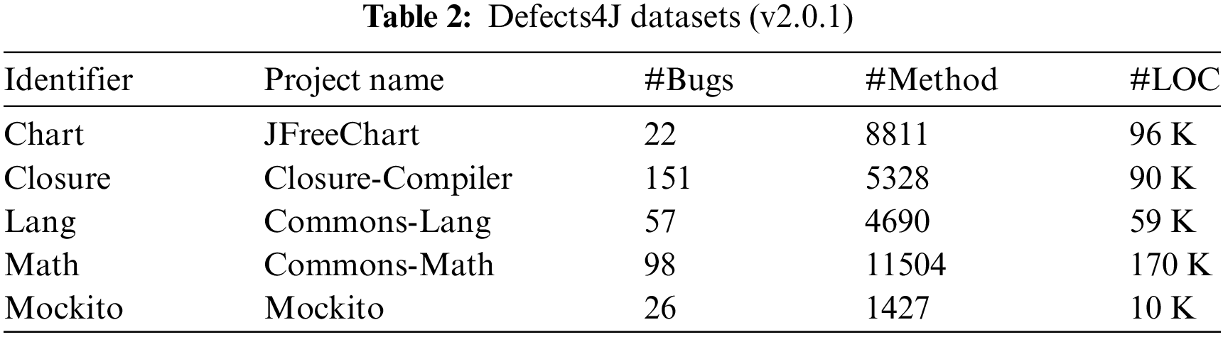
This paper chooses Defects4J (v2.0.1) benchmark to evaluate the effectiveness of Two-RGCNFL. Defects4J is a widely used dataset in software fault research, which contains a series of real-world software fault projects to evaluate and compare the performance of different fault localization and repair techniques. This paper has utilized 5 open-source Java projects from the Defects4J (v2.0.1) benchmark, including Chart, Closure, Lang, Math and Mockito, which contain 408 real bugs in total. Among these, this paper has considered 354 bugs because the remaining 51 bugs do not reside within any method. Table 2 provides a brief statistical overview of this dataset, where the last two columns are the average number of methods and the average number of lines of code per project, respectively.

The reason we choose this dataset is that it contains data from real-world open-source projects. Not only that, it has been widely used in the field of software fault localization in previous studies. This indicates that the dataset can verify the effectiveness of Two-RGCNFL for real fault localization and facilitate evaluation and comparison with other methods.

4.3 Evaluation Metrics

This paper utilizes widely adopted evaluation metrics in the field of software fault localization: Top-K and mean reciprocal rank (MRR).

Top-K represents that at least one faulty method or statement has been localized among the top k ranked positions. In practice, it is extremely time-consuming to examine all the methods or statements in a faulty program. Considering the limited time and resources, this paper uses Top-K to evaluate Two-RGCNFL. In the experimental design, this paper follows majority of previous studies [3,16,18] by setting K to 1, 3 and 5.

MRR represents the reciprocal rank of each fault among all faulty elements. The MRR of each project is the average of the sum of the reciprocal ranks of all its faults. A higher MRR value indicates better model performance. The MRR is calculated as shown in Eq. (16), where denotes the number of faulty versions of each project and denotes the ranking of fault in the faulty version .

(16)

4.4 Parameters Setting

The experiments are carried out in the hardware environment of Intel Core i5-12490F, NVIDIA GeForce RTX4060 8 G and 32 G*2 dual-channel memory, and implemented in the software environment of Python3.8 and PyTorch2.0. For all models, the learning rate is initialized to 0.001, the dropout is set to 0.1, the default epoch is 100, and the Adam optimizer is used for training. In unbalanced processing, since the number of majority samples and minority samples changes according to the actual situation of the project, the imbalance ratio is not set in the experiment, the over-sampling ratio is set to , and the number of MLP hidden layers in the edge generator is set to 2. In the Phase 1 classification model, the data set is randomly divided, the ratio of training set and test set is set to 8:2, and the experiment is repeated three times using cross validation to take the average result. In the ranking model in Phase 2, words with embedding vector size of 100 are used to train the Doc2Vec model.

5  Analysis of Results

5.1 RQ1: What Is the Performance of Two-RGCNFL?

The first phase of Two-RGCNFL implements classification at the method level and the second phase implements ranking at the statement level. This paper will evaluate the performance of the model in these two phases separately. For different fault versions of each project, after processing into the pruned MCDG, the nodes will coincide. As such, in Phase 1, this paper performs cross-validation on the faults of each project. To ensure the accuracy of the statement-level ranking in Phase 2, this paper employs leave-one-out cross validation to evaluate the effectiveness of Two-RGCNFL in statement-level localization. In addition, for RQ1, we compare the Top-K (K = 1, 3, 5) and MRR two measures, using to calculate the percentage improvement of Two-RGCNFL.

5.1.1 RQ1.1: How Accurate Is Two-RGCNFL Localization at the Method Level?

In order to measure the effectiveness of Two-RGCNFL in method-level localization, the following three method-level fault localization methods are used for comparison:

(1) GRACE [18] is a coverage-based localization technique that leverages coverage information thoroughly by constructing a graph representation of the program, and employ graph neural networks to rank faults.

(2) CNN-FL [15] is a fault localization method based on convolutional neural network, which evaluates the suspicion of each program entity by testing the trained model with a virtual test set.

(3) DEEPRL4FL [13] is a deep learning method that classifies faults by treating fault localization as an image pattern recognition problem.

Fig. 4 shows the performance between the proposed Two-RGCNFL and the three baseline methods in terms of method-level fault localization in the overall case. As can be seen from the figure, Two-RGCNFL consistently outperforms all baseline methods on Top-K (K = 1, 3, 5). Specifically, Two-RGCNFL improves by 30~94, 36~102 and 39~92 faults over the baseline methods on Top-K (K = 1, 3, 5), respectively. On the whole, our approach can locate 290 faults on Top-5, accounting for 81.92% of the total number of faults in the experiment. It is effectively verified that Two-RGCNFL can locate more faults at the top of the list in Phase 1.

Figure 4: Comparison of different techniques for method-level fault localization on Top-K (K = 1, 3, 5)

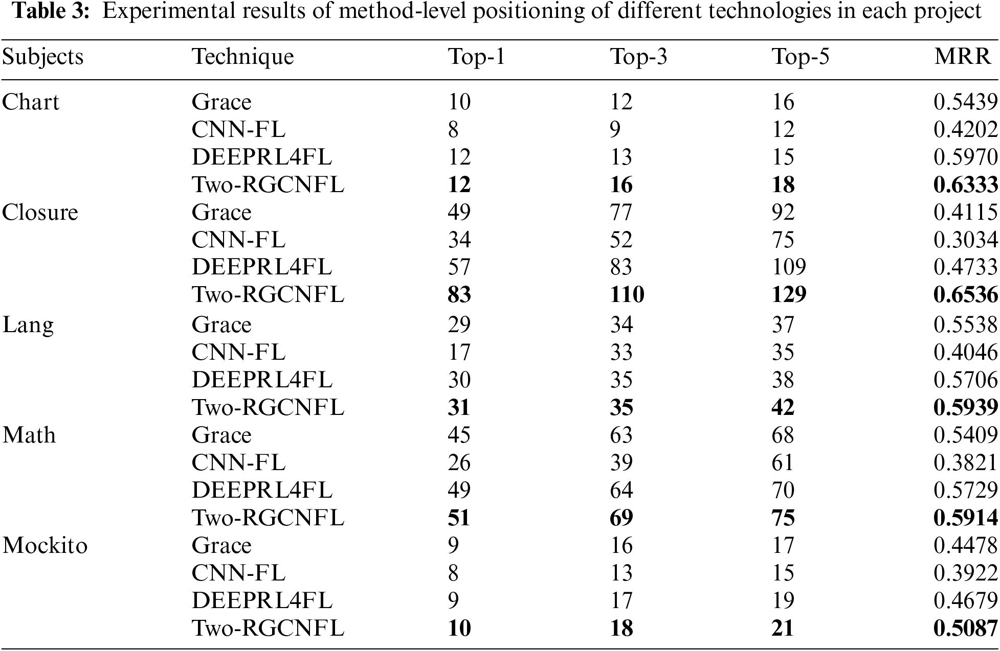
Next, this paper will explore the impact of different projects on the performance of Two-RGCNFL. From Table 3, it can be observed that Two-RGCNFL exhibits the best performance across all projects. In particular, Two-RGCNFL demonstrates significant improvement over CNN-FL. This is because CNN-FL is a deep learning method that relies on test cases to train convolutional neural networks, which makes full use of code coverage information, but ignores the role of code context. Furthermore, we notice that Two-RGCNFL improves the best in the most complex Closure project. Compared with the baseline methods, Two-RGCNFL improves the Top-K (K = 1, 3, 5) accuracy by 45.61%~144.12%, 32.53%~111.54%, and 18.35%~72%, respectively. Notably, the most pronounced improvement is seen at Top-1, indicating that for the Closure project, Two-RGCNFL can localize 54.97% of faults by examining just one method. At the same time, the MRR score increases by 38.09% compared to DEEPRL4FL, the best performing in the baseline method, whereas the improvement in the Math project is only 3.23%. This indicates that Two-RGCNFL has greater confidence in handling complex projects.

5.1.2 RQ1.2: How Accurate Is Two-RGCNFL Localization at the Statement Level?

In order to measure the effectiveness of Two-RGCNFL in statement-level localization, the following two classical SBFL techniques and two statement-level fault localization methods are used for comparison:

(1) SupConFL [3] combines AST with statement sequence, and extracts the features of buggy code through contrastive learning. It employs an attention-based LSTM to locate faulty elements.

(2) LLMAO [16] is a localization technique based on a language model, which is capable of localizing faulty elements without any test coverage information.

(3) Ochiai [27] and Dstar [26] are two classical spectrum-based fault localization techniques, which have been widely used in previous research works.

Fig. 5 shows the performance between the proposed Two-RGCNFL and the four baseline methods in terms of statement-level fault localization in the overall case. As can be seen from the figure, Two-RGCNFL consistently outperforms all baseline methods on Top-K (K = 1, 3, 5). Compared with the traditional SBFL techniques (Ochiai and Dstar), Two-RGCNFL improves the Top-1 accuracy by 262.86%. This is because the traditional SBFL techniques only rely on the program execution spectra to calculate the suspicious values of the statement, neglecting the role of the program’s internal code context. Additionally, the issue of numerous identical suspiciousness values significantly affects the accuracy of ranking. Compared with the two baseline methods (i.e., SupConFL and LLMAO), Two-RGCNFL locates 29 and 44 more faults at Top-1. And at Top-5, it can locate 221 faults, accounting for 64.2% of the total number of faults in the experiment. This result indicates that with a fixed number of inspections, Two-RGCNFL can locate more faulty statements than other methods, effectively saving developers time and effort.

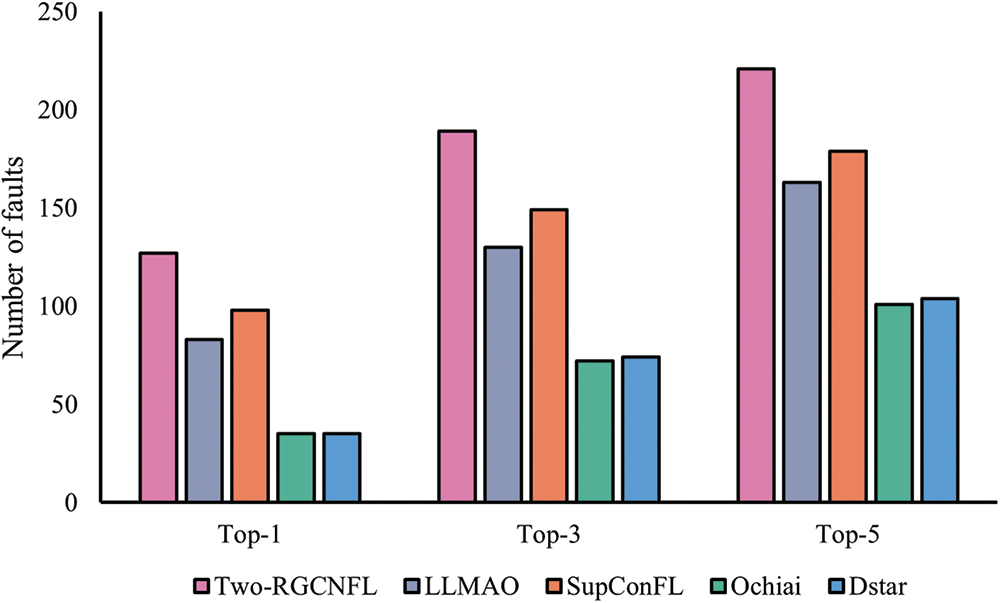
Figure 5: Comparison of different techniques for statement-level fault localization on Top-K (K = 1, 3, 5)

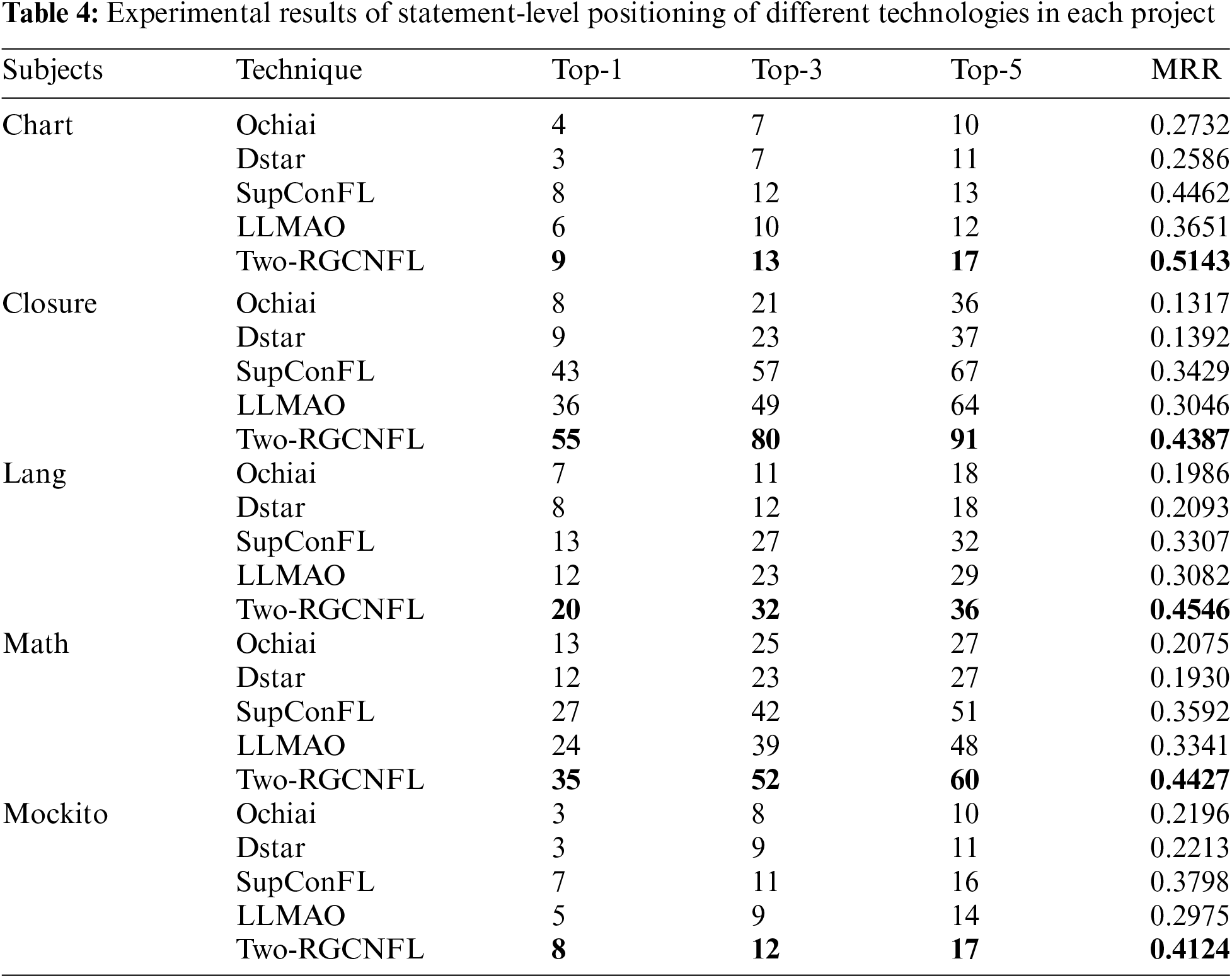
Table 4 shows the performance of different technologies in statement-level localization across various projects. We observe that the traditional SBFL technology exhibits the poorest performance in all projects. One of the key reasons is that they only consider the coverage information of test cases to the code, and assign identical suspiciousness scores to statements within the same basic block. This limitation is particularly evident in more complex projects like Closure, where the MRR decreases by 51.79% and 46.17% respectively compared to the better-performing Chart project. Secondly, LLMAO performs better than the traditional SBFL technique in all projects. For example, in the Math project, LLMAO achieves average improvements of 92.31%, 62.78%, and 77.78% in Top-K (K = 1, 3, 5) accuracy, respectively. This is attributed to the fact that the representations learned by the pre-trained language model already encapsulate extensive knowledge about suspiciousness of the statement, which allows it to locate the fault without executing any test cases. However, this also prevents it from achieving optimal performance. Finally, compared with SupConFL, the best performing method among all baseline methods, Two-RGCNFL improves the Top-K (K = 1, 3, 5) accuracy by 12.5%~53.85%, 8.33%~40.35% and 9.09%~35.82% respectively in all projects. It improves the MRR score by 8.58%~37.47%. The reason why SupConFL works best among the baseline methods is that it can learn richer features of faulty elements. However, only the static information of the code is contained in this feature. In contrast, Two-RGCNFL uses both static and dynamic information of code, and Phase 2 of Two-RGCNFL is based on Phase 1. The completion of Phase 1 greatly reduces the location range of faulty statements for Phase 2, so Two-RGCNFL achieves even better performance.

5.2 RQ2: Does the Construction of MCDG Contribute to the Localization of Two-RGCNFL at the Method Level, and What Extent Can It Bring Benefits?

Although the ultimate goal of this paper is to achieve statement-level localization, the accuracy of method-level localization serves as a prerequisite for the accuracy of statement-level localization. Therefore, this paper has compared the effectiveness of MCDG at the method level. In this paper, a comparison is made by constructing a PDG without inter-class dependencies. In the following, we use MCDG and PDG to denote the construction of MCDG and PDG in Phase 1, respectively.

For RQ2, this paper still adopts Top-K (K = 1, 3, 5) and MRR as the evaluation metric. As can be seen from Fig. 6, MCDG outperforms PDG in both two evaluation metrics. Specifically, MCDG improves Top-K (K = 1, 3, 5) accuracy by 15.91%~40.68%, 20.67%~30.19% and 11.76%~31.25%, respectively, and improves MRR score by 12.56%~32.79%. It is worth noting that from Fig. 3d, we find that MCDG has the most obvious improvement compared with PDG in the Closure project, while it is relatively gentle in the Math project. It indicates that the performance improvement of MCDG varies according to the number of inter-class faults contained in the project. Thus, by additionally considering inter-class dependency relations, fault localization performance can be enhanced to a certain extent, which also demonstrates that the construction of MCDG is effective.

Figure 6: PDG and MCDG are constructed in Two-RGCNFL for comparative experiments. (a) Their performance comparison on Top-1; (b) Their performance comparison on Top-3; (c) Their performance comparison on Top-5; (d) Their performance comparison on MRR

5.3 RQ3 How Does the Number of Hidden Layers of the MLP Affect the Statement Level Localization of Two-RGCNFL in the Modified GraphSMOTE?

In the improved GraphSMOTE algorithm, the feature extractor and edge generator are the main components, and their performance will directly affect the performance of the classification model in Phase 1, and indirectly affect the performance of the ranking model in Phase 2. In the experiment, they are trained by . In Section 3.1.3, is obtained by calculating the error of the actual adjacency matrix and the adjacency matrix predicted by the edge generator, MLP is the main framework structure of the edge predictor, so this paper needs to discuss the number of hidden layers of MLP. In the experiment, is set to {1, 2, 3, 4} to observe the statement-level fault localization performance.

For RQ3, Fig. 7 presents the experimental results for the local Top-1 accuracy and the overall MRR ranking. From the figure, we can see that for five projects, Two-RGCNFL shows the worst localization performance when is 1. This is because when using a shallow network, MLP cannot effectively learn the mutual contributions between nodes and the complex relationships between them, which leads to large errors in the predicted edges, resulting in poor localization results. When is increased to 2, we can find that the localization performance of Two-RGCNFL is improved on different projects. Specifically, the improvement is most obvious on the Closure project, which shows that for complex projects, the increase in the number of hidden layers enables MLP to show its advantages. However, as increases from 2 to 4, the localization performance of Two-RGCNFL begins to decline, and the model will overfit at this time, and the complex relationship between nodes learned may contain a lot of noise, while ignoring more general features or rules. Therefore, in the subsequent task of this work, we fix the number of MLP hidden layers of the edge generator to 2.

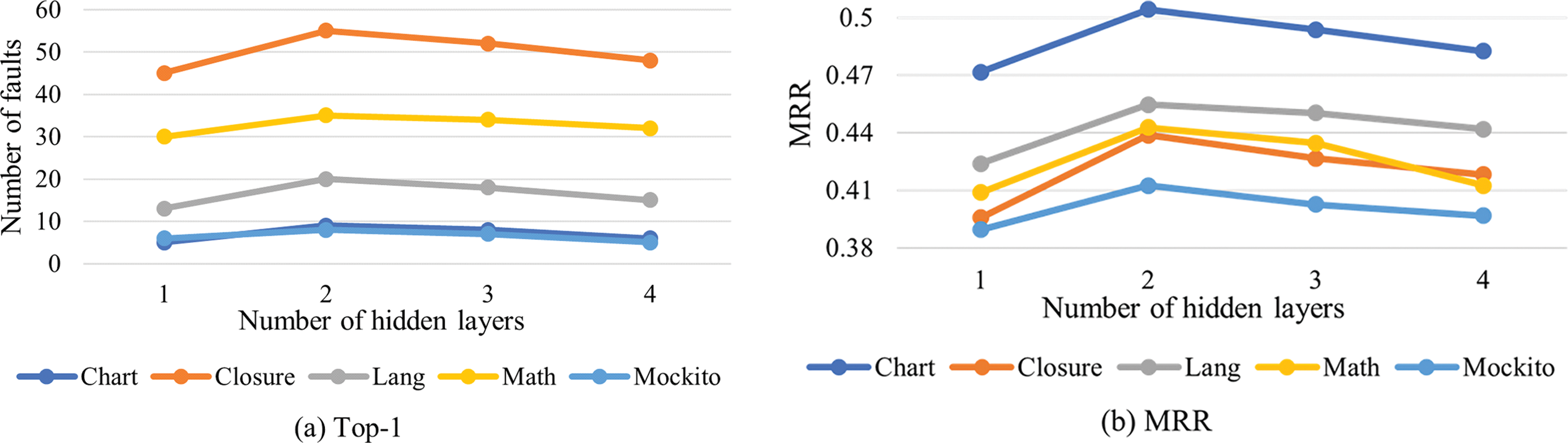
Figure 7: Influence of the number of hidden layers of MLP on Two-RGCNFL (a) comparison of different numbers of hidden layers in Top-1 (b) comparison of different numbers of hidden layers in MRR

5.4 RQ4: What Is the Impact of Different Loss Functions on the Localization of Two-RGCNFL at the Statement Level?

The commonly used loss function in RankNet is the cross-entropy loss function. However, as mentioned in Section 3.3, the features of statements in the same basic block may be very similar, which means that a pair of similar statement features will get very close scores when input into RankNet. This results in the cross-entropy loss function having difficulty distinguishing between them. Therefore, this paper uses hinge loss function in our ranking model. To validate this idea, we conduct a comparison between these two loss functions.

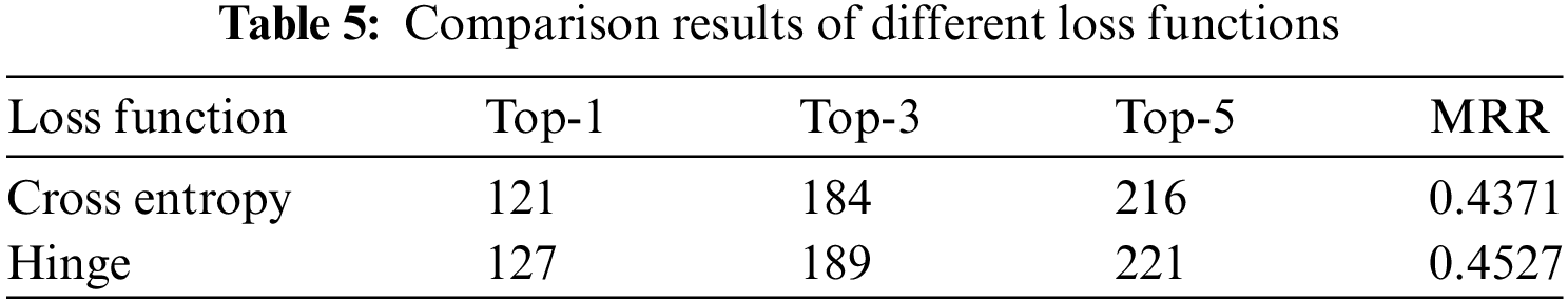
Table 5 presents the experimental results using different loss functions. As can be observed from the table, the hinge loss function outperforms the cross-entropy loss function when used in the ranking model. Specifically, employing the hinges loss function achieved 35.88%, 53.39%, and 62.43% accuracy in Top-K (K = 1, 3, 5), while using the cross-entropy loss function achieved 34.18%, 51.98%, and 61.02% accuracy in Top-K (K = 1, 3, 5). In terms of the MRR score, the hinge loss function improves by 0.0156 compared to the cross-entropy loss function. These data suggest that, although the improvement from using the hinge loss function over the cross-entropy loss function in our approach is modest, it can still aid in localization to a certain extent. It also indicates that the hinge loss function has a stronger discrimination ability for statements with high pairwise similarity in our task.

6  Discussion

6.1 Statistical Significance Test

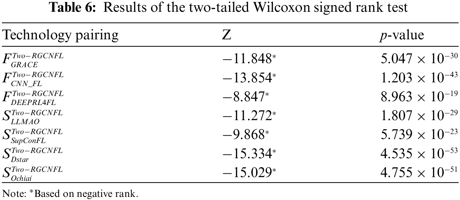
This section discusses whether there is a significant difference between the fault localization performance of Two-RGCNFL and the baseline methods by performing statistical significance tests. We used Wilcoxon signed ranks test for this task because the sample data of this work did not satisfy normal distribution and nonparametric techniques should be chosen to test the data. Wilcoxon signed ranks test is a nonparametric test used to compare the median differences of two related samples. In this paper, the localization results of Two-RGCNFL are set as the front data, and the localization results of other baseline methods are set as the back data. The null hypothesis is that there is no significant difference between the localization performance of Two-RGCNFL and the baseline methods. The alternative hypothesis is a significant difference between the localization performance of Two-RGCNFL and the baseline methods. In addition, two-tailed test is used in the experiment.

The significance experiment considers 354 faults of Defects4J dataset, applying different techniques to rank each fault. Wilcoxon signed ranks test is used to confirm the difference between the two groups of ranking results. As shown in Table 6, represents the significance test of localization results of techniques and at the method level, and represents the significance test of localization results of techniques and at the statement level. The table shows that the p-values for all pairs are extremely small, so the null hypothesis is rejected and the alternative hypothesis is accepted at a significance level greater than 99%. That is, there is a statistically significant difference between the localization performance of Two-RGCNFL and the baseline methods.

6.2 Threats to Validity

Threats to internal validity are mainly feature collection. Feature collection involves the integrity of the datasets and the correctness of the tools. This paper uses Doc2Vec and Gzoltar to extract the semantic information and spectral information of the programs, respectively. Both of these tools have been verified by the majority of researchers and are widely used in various applications.

Threats to external validity are mainly from the dataset. The dataset used in our experiments is 5 projects from the Defects4J (v2.0.1) benchmark. In the future, we will conduct experiments using different datasets to verify the generality of our approach. In addition, Defects4J is a dataset based on Java language, which limits the universality and applicability of the experimental results to a certain extent. Firstly, the Java language has its unique syntax and runtime features, which may make the proposed approach challenging when applied to other programming languages. Secondly, in the proposed method, the construction of MCDG is a key step, and in this work, the Soot tool is used to build MCDG. Soot is a bytecode analysis framework designed specifically for Java. Its functions and optimization strategies are closely centered on the features of Java language. Therefore, it may be necessary to find or develop similar code analysis tools when applying the methods of this study to other programming languages. In the future, we will choose a variety of representative programming languages, such as C++ or Python, etc. For these programming languages, explore and develop code analysis tools or alternatives suitable for these languages. Thus, the generality and applicability of the proposed method can be more comprehensively evaluated.

7  Conclusion and Future Work

This paper introduces Two-RGCNFL, a deep learning approach that integrates inter-class and intra-class dependencies into MCDG, and then uses RGCN to extract node features of MCDG, which enables it to locate inter-class method call type faults. In addition, this paper uses the RankNet model to address the issue of equal suspicious values of statements within the same basic block. The experimental results demonstrate that Two-RGCNFL significantly outperforms traditional SBFL techniques in statement-level fault localization, and it maintains its superiority compared to other baseline methods presented in this paper. Furthermore, this paper experimentally demonstrates that additionally considering inter-class method dependencies gives better results than only considering intra-class method dependencies. In the future, for Phase 1, we will investigate the construction of MCDG on different programming languages to enhance the applicability of Two-RGCNFL. For Phase 2, in the feature extraction module, we will study the impact of other different feature dimensions on localization performance, aiming to maximize localization performance.

Acknowledgement: The authors would like to express our sincere appreciation to the Youth Fund of the National Natural Science Foundation of China for their financial support. We would like to thank the School of Software, Nanchang Hangkong University for providing resources for this research.

Funding Statement: This research was funded by the Youth Fund of the National Natural Science Foundation of China (Grant No. 42261070).

Author Contributions: The authors confirm contribution to the paper as follows: study conception and design: Xin Fan, Zhenlei Fu, Jian Shu; data collection: Zhenlei Fu, Zuxiong Shen; analysis and interpretation of results: Xin Fan, Zhenlei Fu, Jian Shu; draft manuscript preparation: Xin Fan, Zhenlei Fu, Zuxiong Shen, Yun Ge; fund support: Yun Ge. All authors reviewed the results and approved the final version of the manuscript.

Availability of Data and Materials: The data that support the findings of this study are openly available in https://github.com/Jan0813/Two-RGCNFL/tree/master (accessed on 06 November 2024).

Ethics Approval: Not applicable.

Conflicts of Interest: The authors declare no conflicts of interest to report regarding the present study.

References

1. Y. Du and Z. Yu, “Pre-training code representation with semantic flow graph for effective bug localization,” in Proc. 31st ACM Joint ESEC/FSE, New York, NY, USA, 2023, pp. 579–591. [Google Scholar]

2. H. Wang et al., “Can higher-order mutants improve the performance of mutation-based fault localization?” IEEE Trans. Reliab., vol. 71, no. 2, pp. 1157–1173, 2022. doi: 10.1109/TR.2022.3162039. [Google Scholar] [CrossRef]

3. W. Chen, W. Chen, J. Liu, K. Zhao, and M. Zhang, “SupConFL: Fault localization with supervised contrastive learning,” in Proc. 14th Asia-Pacific Sym. Internetware, New York, NY, USA, 2023, pp. 44–54. [Google Scholar]

4. J. Qian, X. Ju, and X. Chen, “GNet4FL: Effective fault localization via graph convolutional neural network,” Autom. Softw. Eng., vol. 30, no. 2, 2023, Art. no. 16. doi: 10.1007/s10515-023-00383-z. [Google Scholar] [CrossRef]

5. Y. Ma and M. Li, “The flowing nature matters: Feature learning from the control flow graph of source code for bug localization,” Mach. Learn., vol. 111, no. 3, pp. 853–870, 2022. doi: 10.1007/s10994-021-06078-4. [Google Scholar] [CrossRef]

6. Z. Zhang, Y. Lei, X. Mao, M. Yan, X. Xia and D. Lo, “Context-aware neural fault localization,” IEEE Trans. Softw. Eng., vol. 49, no. 7, pp. 3939–3954, 2023. doi: 10.1109/TSE.2023.3279125. [Google Scholar] [CrossRef]

7. Y. Yan, S. Jiang, Y. Zhang, S. Zhang, and C. Zhang, “A fault localization approach based on fault propagation context,” Inf. Softw. Technol., vol. 160, 2023, Art. no. 107245. doi: 10.1016/j.infsof.2023.107245. [Google Scholar] [CrossRef]

8. Y. Li and P. Liu, “A preliminary investigation on the performance of SBFL techniques and distance metrics in parallel fault localization,” IEEE Trans. Reliab., vol. 71, no. 2, pp. 803–817, 2022. doi: 10.1109/TR.2022.3165195. [Google Scholar] [CrossRef]

9. M. Zhang et al., “An empirical study of boosting spectrum-based fault localization via PageRank,” IEEE Trans. Softw. Eng., vol. 47, no. 6, pp. 1089–1113, 2021. doi: 10.1109/TSE.2019.2911283. [Google Scholar] [CrossRef]

10. G. Zhao, H. He, and Y. Huang, “Fault centrality: Boosting spectrum-based fault localization via local influence calculation,” Appl. Intell., vol. 52, no. 7, pp. 7113–7135, 2022. doi: 10.1007/s10489-021-02822-4. [Google Scholar] [CrossRef]

11. R. Widyasari, G. A. A. Prana, S. A. Haryono, Y. Tian, H. N. Zachiary and D. Lo, “XAI4FL: Enhancing spectrum-based fault localization with explainable artificial intelligence,” in Proc. 30th IEEE/ACM Int. Conf. Program Comprehension, New York, NY, USA, 2022, pp. 499–510. [Google Scholar]

12. D. Callaghan and B. Fischer, “Improving spectrum-based localization of multiple faults by iterative test suite reduction,” in Proc. 32nd ACM SIGSOFT Int. Sym. Softw. Testing Anal., New York, NY, USA, 2023, pp. 1445–1457. [Google Scholar]

13. Y. Li, S. Wang, and T. Nguyen, “Fault localization with code coverage representation learning,” in IEEE/ACM 43rd Int. Conf. Softw. Eng., Madrid, Spain, 2021, pp. 661–673. [Google Scholar]

14. J. Cao et al., “DeepFD: Automated fault diagnosis and localization for deep learning programs,” in Proc. 44th Int. Conf. Softw. Eng., New York, NY, USA, 2022, pp. 573–585. [Google Scholar]

15. Z. Zhang, Y. Lei, X. Mao, and P. Li, “CNN-FL: An effective approach for localizing faults using convolutional neural networks,” in IEEE 26th Int. Conf. SANER, Hangzhou, China, 2019, pp. 445–455. [Google Scholar]

16. A. Z. H. Yang, C. Le Goues, R. Martins, and V. Hellendoorn, “Large language models for test-free fault localization,” in Proc. IEEE/ACM 46th Int. Conf. Softw. Eng., New York, NY, USA, 2024, pp. 1–12. [Google Scholar]

17. X. Meng, X. Wang, H. Zhang, H. Sun, and X. Liu, “Improving fault localization and program repair with deep semantic features and transferred knowledge,” in Proc. 44th Int. Conf. Softw. Eng., New York, NY, USA, 2022, pp. 1169–1180. [Google Scholar]

18. Y. Lou et al., “Boosting coverage-based fault localization via graph-based representation learning,” in Proc. 29th ACM Joint Meeting ESEC/FSE, New York, NY, USA, 2021, pp. 664–676. [Google Scholar]

19. X. Gou, A. Zhang, C. Wang, Y. Liu, X. Zhao and S. Yang, “Software fault localization based on network spectrum and graph neural network,” IEEE Trans. Reliab., pp. 1–15, 2024. doi: 10.1109/TR.2024.3374410. [Google Scholar] [CrossRef]

20. M. N. Rafi, D. J. Kim, A. R. Chen, T. P. Chen, and S. Wang, “Towards better graph neural network-based fault localization through enhanced code representation,” in Proc. ACM Softw. Eng., New York, NY, USA, 2024, pp. 1937–1959. [Google Scholar]

21. A. Mantovani, A. Fioraldi, and D. Balzarotti, “Fuzzing with data dependency information,” in 2022 IEEE 7th Eur. Sym. Secur. Priv. (EuroS&P), 2022, pp. 286–302. [Google Scholar]

22. A. V. Karuthedath, S. Vijayan, and K. S. Vipin Kumar, “System dependence graph based test case generation for object oriented programs,” in 2020 Int. Conf. Power, Instrum. Control Comput. (PICC), 2020, pp. 1–6. [Google Scholar]

23. L. L. Wang, B. X. Li, and X. L. Kong, “Type slicing: An accurate object oriented slicing based on sub-statement level dependence graph,” Inf. Softw. Technol., vol. 127, 2020, Art. no. 106369. doi: 10.1016/j.infsof.2020.106369. [Google Scholar] [CrossRef]

24. T. Zhao, X. Zhang, and S. Wang, “GraphSMOTE: Imbalanced node classification on graphs with graph neural networks,” in Proc. 14th ACM Int. Conf. Web Search Data Min., New York, NY, USA, 2021, pp. 833–841. [Google Scholar]

25. Q. Le and T. Mikolov, “Distributed representations of sentences and documents,” in Proc. 31st Int. Conf. Mach. Learn., Beijing, China, 2014, pp. 1188–1196. [Google Scholar]

26. W. E. Wong, V. Debroy, R. Gao, and Y. Li, “The DStar method for effective software fault localization,” IEEE Trans. Reliab., vol. 63, no. 1, pp. 290–308, 2014. doi: 10.1109/TR.2013.2285319. [Google Scholar] [CrossRef]

27. R. Abreu, P. Zoeteweij, and A. J. C. Van Gemund, “An evaluation of similarity coefficients for software fault localization,” in 12th Pacific Rim Int. Symp. Depend. Comput. (PRDC'06), Riverside, CA, USA, 2006, pp. 39–46. [Google Scholar]

28. R. Dharanappagoudar, P. Gupta, and S. Godboley, “CMHFL: A new Fault Localization technique based on Cochran–Mantel–Haenszel method,” in 2022 IEEE 19th India Council Int. Conf. (INDICON), Kochi, India, 2022, pp. 1–7. [Google Scholar]

29. N. V. Chawla, K. W. Bowyer, L. O. Hall, and W. P. Kegelmeyer, “SMOTE: Synthetic minority over-sampling technique,” J. Artif. Intell. Res., vol. 16, pp. 321–357, 2002. doi: 10.1613/jair.953. [Google Scholar] [CrossRef]

30. M. A. K. T. Schlichtkrull, “Modeling relational data with graph convolutional networks,” in The Semantic Web. Cham: Springer, 2018, pp. 593–607. [Google Scholar]

31. Y. Lecun, Y. Bengio, and G. Hinton, “Deep learning,” Nature, vol. 521, no. 7553, pp. 436–444, 2015. doi: 10.1038/nature14539. [Google Scholar] [PubMed] [CrossRef]

32. C. Burges et al., “Learning to rank using gradient descent,” in Proc. 22nd Int Conf. Mach. Learn., New York, NY, USA, 2005, pp. 89–96. [Google Scholar]