ACSF-ED: Adaptive Cross-Scale Fusion Encoder-Decoder for Spatio-Temporal Action Detection

1  Introduction

Spatio-Temporal Action Detection (STAD) is a crucial task in video understanding as it aims to locate the actor in space and classify the actions performed by the actor over time. This line of research finds applications in various fields, including the detection of workers’ abnormal safety behaviors in factories [1], the detection of illegal actions in public places [2,3], the detection of autonomous driving [4], and the detection of driver actions [5]. The existing methods proposed [6–8] all focus on enhancing the detection performance of human actions. Therefore, improving the learning and comprehension capabilities of detection models becomes a current research focus.

Currently, deep learning-based STAD can be categorized into two types based on the prediction form in the proposal: clip-level detection and frame-level detection.

1.1 Clip-Level Detection

The clip-level detection method is designed to extract 3D spatio-temporal tubelets. These tubelets are temporal and spatial 3D proposals that are obtained from video clips for prediction.

Inspired by Faster Region-based Convolutional Neural Networks (Faster-RCNN), Hou et al. proposed an end-to-end network called Tube Convolutional Neural Network (T-CNN) [9] that expanded 2D proposals to 3D proposals by 3D convolution. Kalogeiton et al. developed an Action Tubelet detector (ACT-Detector) [10] that introduces fixed anchored cuboids based on Single Shot MultiBox Detector (SSD) [11] to classify and regress the frame sequence. The detection methods mentioned above assume that the space range of action tubes is fixed. Those methods do not apply to video clips with large space displacement. Therefore, Yang et al. propose a Spatio-Temporal Progressive Learning framework called STEP [12], which uses spatial refinement to iteratively update bounding boxes. It refines 3D cuboid proposals over time and uses time expansion to adaptively add sequence lengths to obtain more context information. Zhao et al. designed a method called tubelet-transformer (TubeR) [7], which uses tubelet’s attention to allow tubelets to be unrestricted in their spatial location and scale over time without anchors. Li et al. proposed the MovingCenter Detector (MOC-Detector) [13] based on the idea of an anchor-free object detector, and Ma et al. developed the Self-Attention MovingCenter Detector (SAMOC) [14], which introduces a spatio-temporal non-local block using a self-attention mechanism. In addition, Duarte et al. proposed a video capsule network called VideoCapsuleNet [15] to remove anchors and use 3D convolutions and capsules to learn the semantic information. Apart from actions with significant magnitudes, there are some actions that are challenging to define and exhibit high false detection rates, such as actions of transitional states. In response to this scenario, Song and colleagues proposed the Transition-Aware Context Network (TACNet) [16].

It is evident that clip-level detection methods capitalize on the temporal continuity of the video. However, clip-level detection requires the extraction of video slices and only provides an action category for predicted spatio-temporal object tubelets, instead of assigning an action classification to each frame. This poses challenges in achieving frame-level precision classification.

1.2 Frame-Level Detection

Thus, there is another method. We know that object detection is also an image detection task. Therefore, it can be applied to STAD. Referring to the methods of object detection, frame-level action detection generates 2D proposals for action actors for each frame in the video, and subsequently classifies the action.

The traditional approach for frame-level spatio-temporal action detection is to directly determine the action object and category of each frame using object detection. The model based on R-CNN proposed by Gkioxari et al. [17] serves as the foundation for the development of the frame-level approach. The network obtains the Region of Interest (RoI) and then employs a dual-flow architecture to extract appearance features and motion features from RGB images and optical flows, respectively. Finally, a support vector machine is used to classify these features. Saha et al. [18] obtain RoI by replacing the unsupervised region proposal algorithm with a region recommendation algorithm and then utilizing a neural network to classify the RoI. In addition, Peng et al. [19] propose a multi-region dual-flow R-CNN model based on Faster R-CNN. The aforementioned methods offer a significant advantage in capturing the appearance information of individual frame images. However, these approaches fail to consider time context information, resulting in inadequate action information content. To address this problem, Yang et al. propose a Cascade Proposal and Location Anticipation (CPLA) model [20] which can infer the motion trend of actions between two consecutive frames. In addition to the optical flow, related researchers use 3D convolution neural networks to directly extract action information in multiple adjacent frames based on video content, simply obtaining spatio-temporal action information and achieving good extraction results. Gu et al. proposed an Interactive three Dimensions (I3D) model [21]. The SlowFast network [6] designed by Feichtenhofer et al. is a novel two-stream architecture consisting of a slow path and a fast path. However, while these methods can obtain better spatio-temporal information, they are affected by the complexity of 3D convolutional neural networks. Therefore, Feichtenhofer et al. designed the X3D network [22], which is similar to the high-resolution Fast Pathway. The network is constructed by incrementally expanding along multiple network axes, including time, space, width, and depth, to a compact 2D architecture. To simplify and unify the network, Chen et al. proposed an end-to-end video action detection framework called Watch Only Once (WOO) [23]. The performance decreases in tandem with the reduction in network complexity. Kopuklu et al. proposed You Only Watch Once (YOWO) [8], a two-branch single-stage network containing 2D-CNN features of key frame extraction and 3D-CNN space-time modeling of fragments. It finally outputs regression frames and action classification results of single frames. YOWOv2 [24] and YOWOv3 [25], building upon the YOWO dual-branch structure, utilize a pyramid structure to extract multi-scale features for capturing subtle motion behaviors. They also employ different architectures to optimize the network model structure. The detection accuracy of the YOWO series network still needs further improvement.

In summary, these STAD methods have demonstrated excellent performance. However, these algorithms may not fully extract spatio-temporal information features comprehensively, potentially missing out on detecting the same action information across different scales. Therefore, there is room for further improvement in detection performance. To address this, we continue to enhance the model’s understanding of behavioral objects based on current research, aiming to improve the model’s interpretative effectiveness for spatio-temporal action.

(1)   We propose an end-to-end Adaptive Cross-Scale Fusion Encoder-Decoder (ACSF-ED) for STAD tasks. This network consists of the ACSF Spatio-Temporal (ST)-Encoder and Shared-Head Decoder. It demonstrates robust representation and comprehension abilities for spatio-temporal action information, thereby enhancing predictive capabilities for actions and their corresponding positions.

(2)   Within the ACSF ST-Encoder, the Asymptotic Cross-scale Feature-fusion Module (ACCFM) is introduced. This module allows each scale to incorporate information weighting from high-level semantic spatial features. As a result, the negative impact of accuracy degradation caused by the deterioration of the highest semantic features is reduced. This information can then be utilized by subsequent decoders for comprehension and learning, thereby promoting the enhancement of detection accuracy.

(3)   Traditional methods often do not process the extracted spatio-temporal feature information thoroughly, and they may lack sufficient constraints during training, resulting in lower prediction accuracy. To address this issue, a shared classification and regression detection head is constructed within the Shared-Head Decoder, upon which a multi-constraint loss function is proposed. These components provide more comprehensive constraints for the model during training, enriching the learning process. As a result, the model’s prediction boxes are closer to the ground truth, improving the hit rate of predicted classification.

(4)   Our model was experimented with the popular UCF101-24 dataset and JHMDB-21 dataset, demonstrating excellent STAD capabilities in mainstream tasks.

2  Related Work

To achieve excellent prediction results in spatio-temporal action detection tasks, it is not only related to the process of feature extraction and fusion but also to the level of understanding of the extracted features during prediction.

Traditional STAD [17,18] extracts and fuses image and video features at a single scale for subsequent analysis and prediction, which can lead to overlooking the recognition of subtle actions and result in suboptimal accuracy in spatio-temporal action detection. To address this issue, many studies have proposed various multi-scale feature extraction methods, such as feature pyramids. Inception [26] utilizes a parallel multi-branch network structure, where branches employ convolution and pooling networks at different scales to obtain features at various scales, which are then fused. Spatial Pyramid Pooling Network (SPP-Net) [27] employs multiple pooling blocks of different sizes to capture distinct feature blocks, which are merged to obtain the required number of features. Pyramid Scene Parsing Network (PSP-Net) [28] ensures the weight information of global features by reducing the dimensionality of extracted features at different dimensions, performing bilinear interpolation on feature maps, and concatenating them as global features for pyramid pooling. These methods often employ parallel structures to obtain and fuse features from different receptive fields within the same level. However, such approaches tend to overlook the relationships between features at different scales. Feature pyramid networks (FPN) [29] uses a top-down approach to integrate high-level features into low-level features, guiding the fusion of low-level feature information. FPN enhances the correlation between features at different scales, yet such associations may still not be comprehensive, potentially leading to information loss during propagation. Therefore, the ASFF network [30] introduces an Adaptive Structure Feature Fusion module to merge multiple feature maps at different levels. In this study, feature extraction only involves self-attention calculations on high-level semantics. Hence, in the top-down fusion process of ACCFM in this paper, an adaptive structure is employed to ensure the integrity of feature information during sequential propagation, enabling the transmission of high-level semantic information to features at other scales. This enhances the encoder network’s feature fusion capabilities and overall feature representation.

The interpretive ability of extracted features is related to the processing structure of the model. STAD methods based on frame-level borrow from image object detection methods. Image object detection typically adopts a two-stage method like the R-CNN [31] series. On the contrary, single-stage methods such as the You Only Look Once (YOLO) series, SSD [11], and Fully convolutional one-stage object detection (FCOS) [32] can obtain prediction results for the input image faster, eliminating the step of Region Proposal Network (RPN). YOLO which is divided into anchor-based [33–35] and anchor-free [36,37] has rapidly developed. Transformer [38] has also started to be applied in images and other fields. Carion et al. proposed an end-to-end detector, Detection Transformer (DETR) [39], based on the transformer. Additionally, networks such as Dynamic Anchor Boxes Detection Transformer (DAB-DETR) [40] and DeNoising Detection Transformer (DN-DETR) [41] have made improvements in training strategies and other aspects. Due to the powerful feature understanding capabilities of DETR’s encoder-decoder, ACSF-ED also utilizes a simplified encoder-decoder structure, replacing the direct convolutional layer predictions of the original frame-level methods.

3  Our Method

The Adaptive Cross-Scale Fusion Encoder-Decoder (ACSF-ED) network, as illustrated in Fig. 1, consists of two main components: the Adaptive Cross-Scale Fusion Spatio-Temporal Encoder (ACSF ST-Encoder) and the Sharded-Head Decoder. The ACSF ST-Encoder comprises a two-branch module and a fusion module (Section 3.1). The upper branch of the two-branch module consists of a 2D Backbone and a 2D Adaptive Cross-Scale Fusion Spatial-Encoder (ACSF S-Encoder) composed of Attention-based Intra-scale Feature Interaction (AIFI) [42] and Asymptotic Cross-scale Feature-fusion Module (ACCFM), while the lower branch extracts 3D video information features using a 3D backbone. The channel fusion module concatenates the 2D features and 3D features extracted from the two branches in the channel dimension for fusion, thus obtaining a feature with temporal and spatial information. The Shared-Head Decoder decodes the feature vector with temporal and spatial information to progressively generate predictions of the position and category of action (Section 3.2). During training, a multi-constraint supervised loss calculation method is employed to impose constraints.

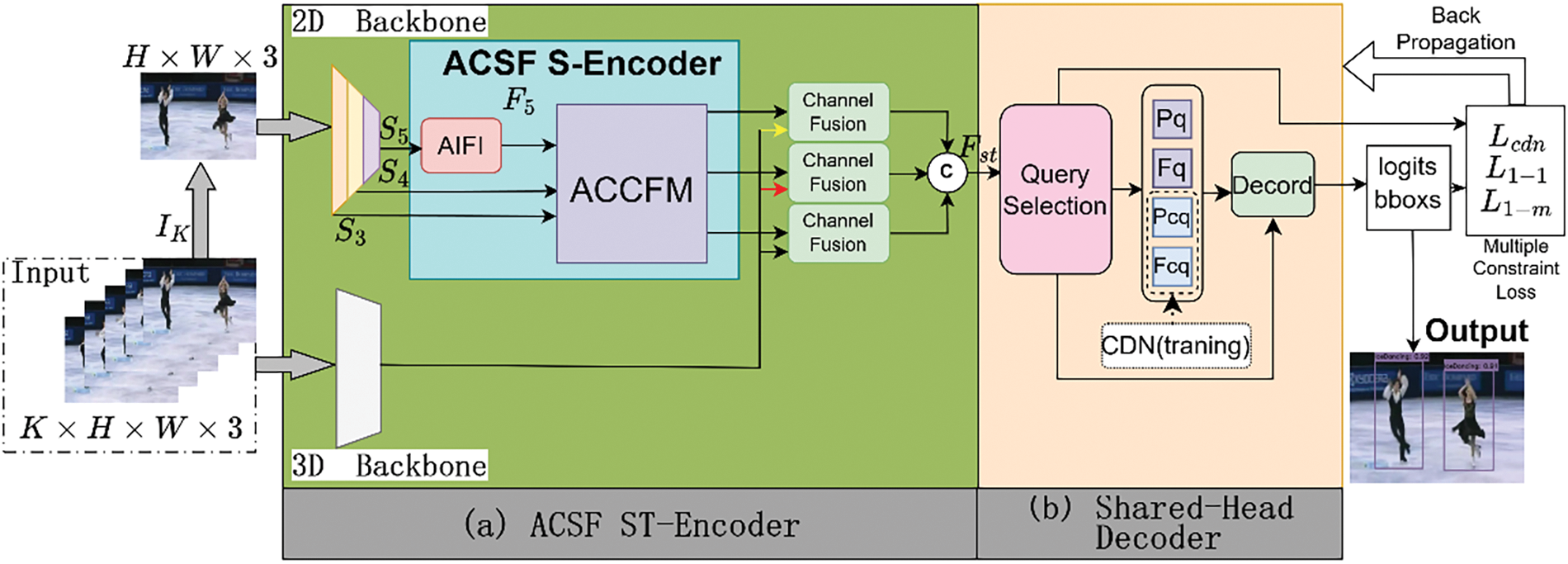
Figure 1: The adaptive cross-scale fusion encoder-decoder (ACSF-ED) network framework

3.1 Adaptive Cross-Scale Fusion Spatio-Temporal Encoder

The Adaptive Cross-Scale Fusion Spatio-Temporal Encoder is a module that integrates features extracted from behavior videos in images with features extracted from videos. This module can capture valuable action and positional information from high-quality behavior videos to be utilized by subsequent modules. The structure of the Adaptive Cross-Scale Fusion Spatio-Temporal Encoder comprises the 2D backbone ResNet [43], the Adaptive Cross-Scale Feature Fusion Spatial-Encoder, the 3D backbone spatio-temporal feature extractor ResNext, and the channel fusion, as depicted in Fig. 2. The 2D backbone analyzes the last frame of the video slice to extract 5-level multi-scale features, denoted as , , , , where the spatial sampling rate between adjacent scale features differs by a factor of 2. To ensure the model’s efficiency and effectiveness, the information-rich and appropriately sized last three scale features , , are selected for input into the ACSF S-Encoder. Due to the fact that the input to the ACSF S-Encoder consists of multi-scale features, improper handling of these features can lead to the spatial encoder becoming overly complex, occupying 49% of the computation load of the encoder-decoder [44]. , , and represent concatenated multi-scale features, and conducting feature interactions on concatenated multi-scale features is somewhat redundant, especially concerning intra-scale feature interaction computations involving self-attention. Intra-scale interactions of low-level features easily duplicate operations and confuse content with interactions of high-level features, making them unnecessary. Therefore, unlike traditional encoders, the ACSF ST-Encoder conducts intra-scale feature interactions only on the highest semantic information , rather than on all , , and . Furthermore, the AIFI reduces the number of self-attention layers from 6 to 1, further lowering computational complexity.

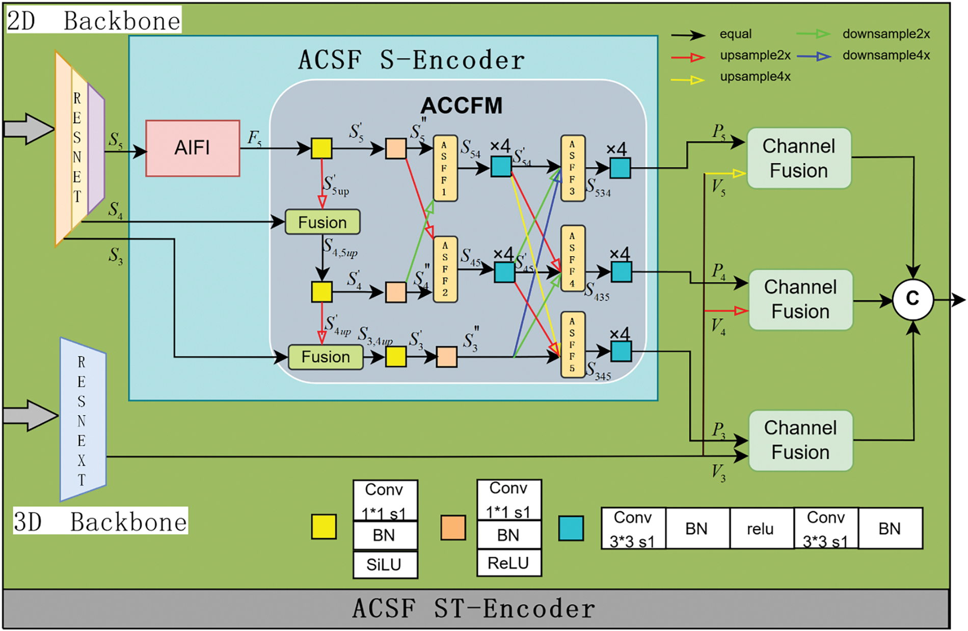
Figure 2: The adaptive cross-scale fusion spatio-temporal encoder (ACSF ST-Encoder) structure

The smallest scale high-level semantic feature is encoded using AIFI to derive . is then propagated to other scales and merged with them through the ACCFM gradually, leading to the extraction of high-quality image feature vectors. The 3D backbone leverages the ResNext-101-3D network [45] to capture spatio-temporal features from the 3D video. The channel fusion concatenates the 2D features and 3D features obtained from the two branches in the channel dimension, followed by convolution and channel self-attention fusion to enable the interactive fusion of spatio-temporal and spatial information, resulting in spatio-temporal features reflecting behavior characteristics.

In the context of this study, the ACCFM module plays a pivotal role in the network. This significance arises from the potential degradation of high-level semantic features during the process of semantic propagation when integrating actions across different scales. Similarly, lower-level semantic features are susceptible to information loss during the propagation phase. This scenario can lead to significant semantic information discrepancies between non-adjacent features, thereby substantially impacting the fusion outcomes. Consequently, the study introduces the ACCFM module. This module functions as a cross-scale fusion network incorporating fusion blocks composed of convolutional layer networks and multiple adaptive structural feature fusion blocks (labeled as , where ranges from 1 to 5). The input to this module comprises multiple scale features, with only the highest semantic feature being subjected to transformer attention operations for acquisition, while the other scale features do not require attention computation, thus alleviating the computational burden. The ACCFM module utilizes an adaptive structural feature fusion block to integrate attention information from the highest semantic features into features at other scales. This allows features at other scales to understand the weight distribution of information across the entire spatial feature, enabling the extraction of high-quality information at different scales.

(1)   Upsampling fusion

The semantic-rich feature extracted from the 2D backbone is enhanced through the AIFI module to derive the high-level feature incorporating attention information. For fusion with the lower-level feature (from the 4th stage), the feature needs to be upsampled to match the size of in subsequent same-size fusion operations. Therefore, undergoes operations including a convolutional layer, BatchNorm layer, and SiLU activation to obtain , as depicted in Eq. (1).

(1)

is upsampled using an interpolation method to obtain the feature at the same scale as , as illustrated in Eq. (2).

(2)

The feature obtained from Eq. (2) and the input are fed into the fusion block, resulting in the fused feature , as shown in Eq. (3).

(3)

The fusion block [42] is a dual-branch structure as illustrated in Fig. 3. Each branch comprises a convolution. The lower branch undergoes N layers of RepBlock processing (typically utilizing 3 layers of RepVgg [46]) after the convolution. Finally, the output feature vectors from both branches are element-wise added together. Assuming the inputs are denoted as and , the process can be represented as shown in Eq. (4):

(4)

where is and is for Eq. (4).

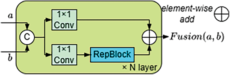
Figure 3: Fusion block structure

If the fused feature obtained from Eq. (3) is to be fused with , it needs to undergo a convolution and a upsampling process to obtain the feature at the same scale as , as described in Eqs. (5) and (6).

(5)

(6)

Subsequently, by fusing and as inputs and into Eq. (4), the feature is obtained as shown in Eq. (7). This feature then undergoes a convolution, Batch Normalization (BN), and SiLU activation operations to derive the feature inputted into the subsequent adaptive network for cross-scale feature propagation and fusion, as depicted in Eq. (8):

(7)

(8)

(2)   Cross-scale feature weight propagation fusion

The semantic gap between non-adjacent hierarchical features is greater than that between adjacent hierarchical features. For instance, the information gap between the bottom feature and the top feature with crucial information is much larger than the gap between and . In the bottom-up fusion approach, the feature enriched with semantic information is obtained through self-attention mechanisms. This feature, when applied to features at other scales, also helps other scale features to effectively focus on the feature positions corresponding to their scales. However, in the previous upsampling fusion propagation process, there may have been a certain degree of degradation in high-level semantic features. To address this, we utilize an asymptotic architecture to gradually propagate the attention weight information of the feature at its scale to all other scale features. Simultaneously, the model, through adaptive methods, determines the weights allocated to each scale during fusion, enabling the features at each scale to incorporate both the attentional feature information from and the attentional information from neighboring scales. This also prevents loss due to information degradation. The implementation process involves the following two steps: feature information extraction and adaptive cross-scale feature propagation fusion.

1)   Feature information extraction

Features , and at different scales undergo a convolution, BatchNorm, and ReLU activation to obtain features , , and for information extraction, as shown in Eq. (9).

(9)

2)   Adaptive cross-scale feature propagation fusion: it primarily corresponds to the process implemented for .

① The processing steps for and

According to the hierarchical architecture arrangement, is initially fused with the feature. The feature undergoes downsampling (convolution) and is merged with the feature in to obtain the feature . Concurrently, the feature undergoes upsampling (convolution combined with bilinear interpolation upsampling) and is fused with the feature in the module to yield the feature . This process is represented by Eqs. (10) and (11).

(10)

(11)

The and modules are adaptive structural feature fusion modules. ACCFM consists of modules. Their task is to learn the weight information corresponding to different-sized feature maps through the network’s learning and to fuse multiple scale features into a new feature map using a weighted fusion calculation method. Taking the fusion module shown in Fig. 2 as an example, the working principle of is introduced as depicted in Fig. 4.

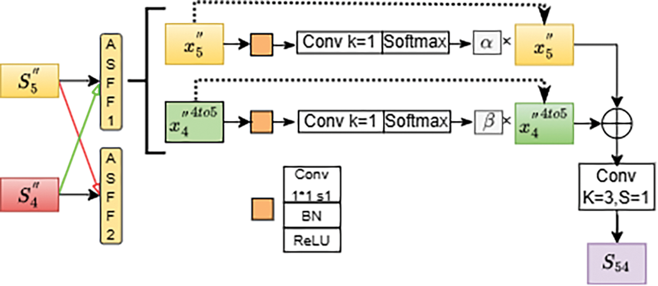
Figure 4: Working principle for

When using ASFF to fuse multiple features, it is necessary to ensure that all the features being fused are at the same scale. This means that features of different scales must be upsampled or downsampled to the same scale before being input into the ASFF module.

In the case of , the inputs are and the features of downsampled by a factor of two, denoted as . The scale of needs to be downsampled in order to match the scale of and generate (i.e., after undergoing downsampling, the scale of matches that of ) for fusion with . Both and are individually processed through a convolutional layer, BatchNorm layer, and ReLU activation, followed by a convolutional layer and Softmax operation to obtain the corresponding weight information and . By multiplying and with the respective original information of and , summing the products, and then passing through a convolution, the new adaptively fused feature is obtained. This process is described by Eq. (12).

(12)

After completing the ASFF operation, the fused feature needs to undergo further processing, including a convolution, BatchNorm, ReLU, another convolution, and BatchNorm, to obtain a new feature. The adaptively fused features and outputted by and respectively undergo the aforementioned steps to obtain and , as shown in Eqs. (13) and (14).

(13)

(14)

② The processing steps for and

Following a similar structure, the feature , the downsampled by a factor of 2 and the downsampled by a factor of 4 are input into the module for fusion to obtain , as described in Eq. (15).

(15)

The feature , the upsampled by a factor of 2 and the downsampled by a factor of 2 are input into the module for fusion to obtain , as described in Eq. (16).

(16)

The feature , the upsampled by a factor of 2 and the upsampled by a factor of 4 are input into the module for fusion to obtain , as described in Eq. (17).

(17)

, , and are further processed through steps involving a convolution, BatchNorm, ReLU, another convolution, and BatchNorm to obtain , and as described in Eqs. (18)–(20).

(18)

(19)

(20)

Detecting an action requires not only identifying the subject of the action but also determining the category of the action. This necessitates features that possess both spatial information to pinpoint the specific location of the object in space and temporal information to imbue the features with clear motion characteristics. The features obtained from the 2D branch, represented as , and , are rich in spatial feature information. Conversely, the multi-scale features , and obtained from the 3D backbone contain spatio-temporal information. This study utilizes an attention-based method [47] to concatenate the acquired 2D spatial features and 3D spatio-temporal features along their corresponding scale-specific features channels at multiple scales, followed by channel-wise concatenation, convolution operation, and channel attention calculation. After processing through the ACSF ST-Encoder, the model obtains spatio-temporal features with characteristics of action.

3.2 Shared-Head Decoder

The purpose of the Shared-Head Decoder proposed in this paper is to interpret the spatio-temporal encoding feature acquired through the ACSF ST-Encoder. It aims to deduce the behavior category and regression position based on this interpreted information. We provide its pseudocode in Algorithm 1 to facilitate a better understanding among readers.

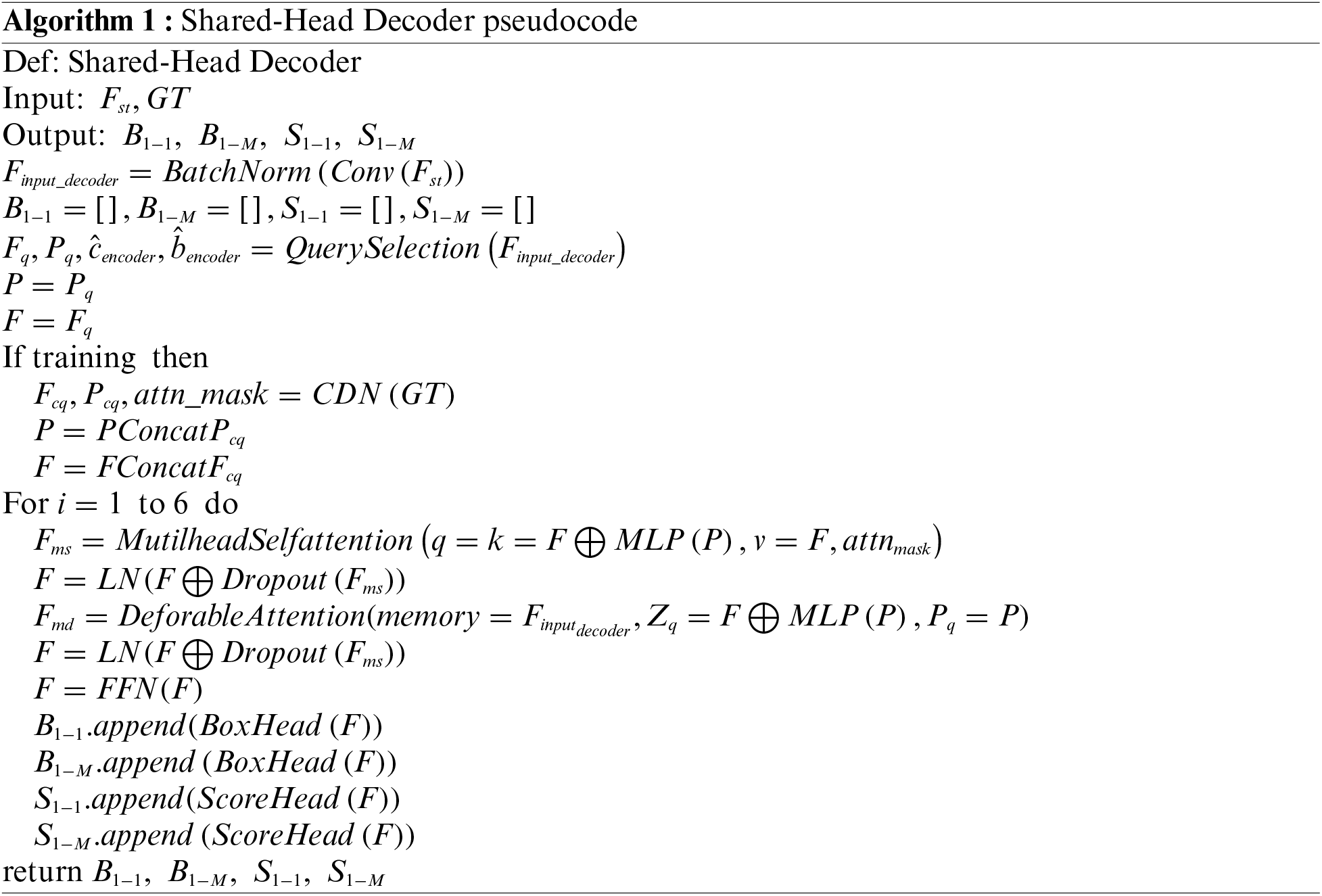
The data acquisition of decoder data involves two parts: Query Selection and Contrastive Denoising (CDN) [48]. Query Selection involves selecting the top-K features with the highest confidence from the output of the ACSF ST-Encoder for Object filtering. The Objects obtained through this process possess enhanced content query () and position query () information. The originally ambiguous “Object Query” has been expanded into two parts: content information and spatial information. Spatial information can be obtained from feature predictions from the encoder layers, while content information can be either statically embedded or dynamically acquired. Given that Object Query now holds practical significance, initializing it improperly can lead to increased training time. Before the selection process, the model passes the output of the last layer of the preceding encoder to a linear layer prediction head to predict confidence levels for each action. The model then selects the top-K (usually defaulting to 300 or 900) feature blocks with the highest classification confidence and records their top-K sequence numbers. The network utilizes the sequence numbers to convey the position predictions (derived from the regression results of the last layer of the encoder through the regression detection head) and the original features of the corresponding feature blocks to the decoder as the content and spatial information for initializing the query objects. The selection of these top-K query objects is constrained by subsequent loss functions (Section 3.2.1), focusing more on objects with high scores and high Intersection over Union (IoU). Before inputting into the decoder, Query Selection can acquire higher-quality query objects by filtering out insignificant ones. This aids in the decoder’s understanding and prediction, simplifying the network computational burden.

During the training phase, CDN generates contrastive denoising noise based on Ground Truth (GT). The task of CDN is to denoise the queries originally input into the decoder, incorporating noisy embeddings of class labels to support label denoising and noisy embeddings of coordinates to support coordinate query denoising, resulting in content queries and position queries . The information is subsequently concatenated with the corresponding queries after Query Selection to generate and . The content queries and position queries are respectively input into the self-attention and cross-attention modules within the decoder layer. CDN actively denoises and combines its corresponding loss function, calculating larger loss for denoised query objects (non-object targets) during training to iteratively update model parameters. Throughout the training, the model gradually improves its predictive capabilities for anchor points without nearby objects and “no-action” objects, enabling active rejective predictions for these objects and enhancing predictive performance. The structure of the Shared-Head Decoder is illustrated in Fig. 5. The main body of the decoder consists of six decoder layers, with each decoder layer comprising a multi-head self-attention mechanism [38] and a cross-attention mechanism [49]. The role of the multi-head self-attention mechanism is to calculate the content query embedding position information and its relationship with itself. Based on this attentional relationship information, the most probable candidate objects are selected, thereby inferring the object position. On the other hand, the cross-attention mechanism utilizes the position query and the output of the multi-head self-attention to further obtain or refine candidate objects. The multi-head self-attention mechanism employs the universal self-attention method used in the transformer. The cross-attention mechanism utilizes a deformable attention mechanism [49] that only interacts with a subset of pixels obtained through sampling. After passing through the self-attention and cross-attention mechanisms, the optimized object candidate objects are input into the Feed Forward Network (FFN) [38] module located in each layer, producing the corresponding output features .

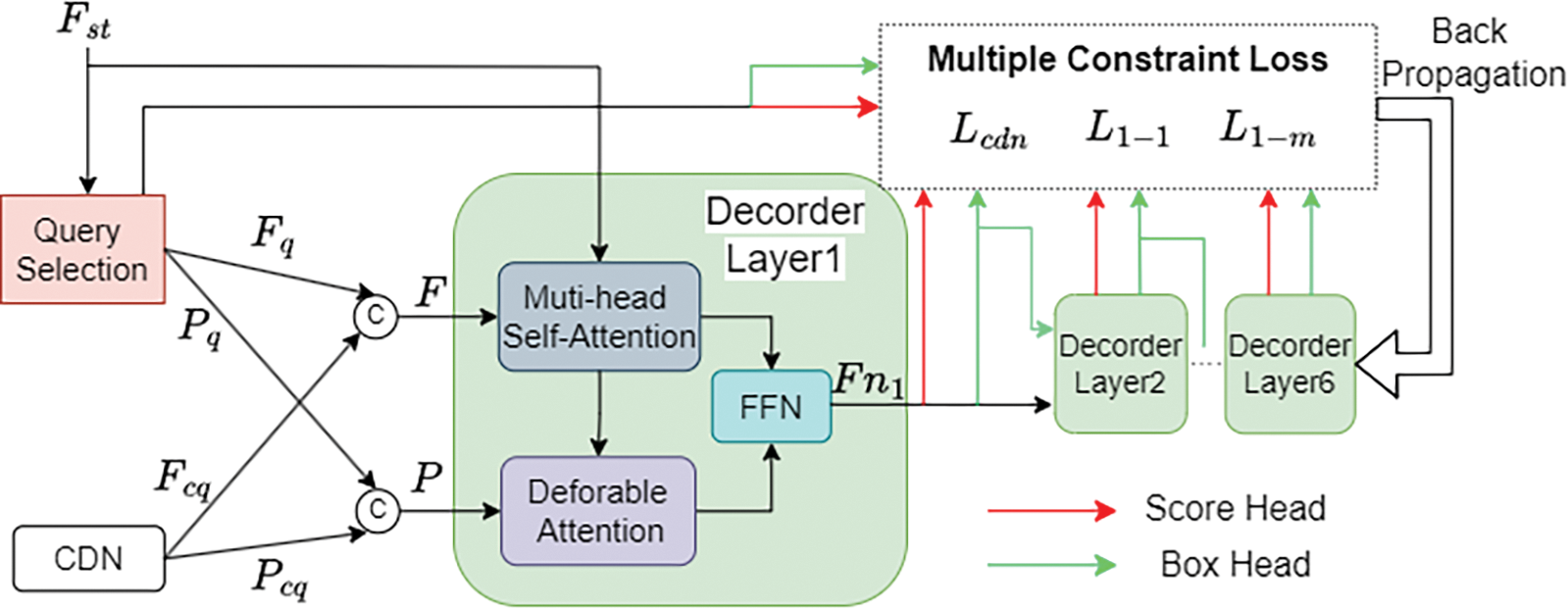
Figure 5: Shared-Head Decoder structure

The results for prediction based on output features necessitate feeding into both one-to-one and one-to-many loss functions. Typically, for these two distinct loss functions, the one-to-one loss function retrieves results from the one-to-one classification and regression detection heads, whereas the one-to-many loss function gathers results from different one-to-many classification and regression detection heads. Moreover, having separate detection heads in all 6 layers of the decoder would increase the computational load. To address this, the Shared-Head Decoder sets the detection heads to be shared, where both the one-to-one and one-to-many loss functions retrieve results from shared classification and regression heads, reducing the original 12 detection heads to 6. At each layer, the output feature is passed to the shared regression head of that layer to predict the coordinates of the behavioral objects, and to the shared classification head to predict confidence scores for multiple behavior categories. The output features and the prediction features of are used as inputs for the next layer . The results obtained from the two shared detection heads in each layer are compared with the GT using multiple loss functions such as , and , which are then incorporated into the final loss calculation. During behavior prediction, the final prediction results are based on the output by the last and . The predictive capabilities of these last two output detection heads are closely linked to various losses mentioned in the next section.

3.2.1 Multi-Constraint Loss Function

The past reliance solely on the one-to-one loss method based on bipartite graph matching has led to shortcomings in the understanding and adequacy of constraints during the learning process of spatio-temporal features by the Encoder-Decoder framework. This often leads to problems in pairing classification and regression, such as assigning high-confidence categories to predictions with low Intersection over Union (IoU) with the GT or to predictions that deviate from the GT objects. In response to this, this paper introduces a multi-constraint supervision method that not only utilizes the CDN method but also incorporates one-to-one and one-to-many supervision methods to enhance training speed and effectiveness, further optimizing the quality of candidate object generation.

In the Shared-Head Decoder, the employs shared and detection heads. After applying different matching algorithms, the one-to-one matching set = ( denotes the optimal permutation of indices) containing prediction results without CDN noise is obtained, along with the set of results from one-to-many matching and the set of prediction results with only CDN noise . In each , the score and box predictions each use a separate prediction head. This approach allows for obtaining prediction results at a lower cost. The one-to-one constrained loss function and the one-to-many constrained loss function are constructed accordingly.

During the training process, it is necessary to compute the corresponding loss function for the predicted results of object query noise by the CDN at each layer, due to the noise introduced by the CDN module before input to the decoder. During training, ACSF-ED will compute the three loss functions , , and for the predictions at each layer, and incorporate them into the overall loss value to enhance constraint supervision. Additionally, the prediction before input to Query Selection in the encoder is also used as an auxiliary loss parameter for one-to-one loss calculation . This leads to the formulation of a multi-constrained loss function , as described in Eq. (21).

(21)

(1)   The one-to-one loss function

The one-to-one constraint loss function completes the loss calculation under a one-to-one bipartite graph matching, where each candidate prediction corresponds to a fundamental ground truth object. In the decoding process, a set of candidate results are already predicted and undergoes a top-K filtering process after the object query passes through Query Selection. This filtering process selects the top-K queries with the highest classification scores, resulting in the selection of the best N queries (N = 300). Among these queries, some may have high classification scores, but if the IoU score between the predicted box and the ground truth box is low, they will be filtered out. Additionally, instances with high IoU scores but not within the top-K range of scores will also be discarded. This significantly impacts the detection performance. To address this issue, the one-to-one constrained loss function is proposed, as shown in Eq. (23). This loss function consists of two parts: the classification loss and the bounding box loss . The calculates the classification loss using the varifocal (VFL) loss function , replacing the Facol loss function, as shown in Eq. (22). introduces the IoU Score [42] to the model, which is “” in the Eq. (22). For positive samples, “q” represents the IoU between the GT classification object and the candidate box, while for negative samples, it defaults to 0. The value “p” denotes the IoU-aware Classification Scores (IACS) value predicted by the model. and are hyperparameters. It employs a loss calculated using IoU to constrain the model to generate high classification scores for features with high IoU and low classification scores for features with low IoU during training. This process aims to provide the decoder with higher quality initial object queries. The component incorporates both L1 loss and Generalized IoU (GIoU) loss to calculate regression loss.

(22)

(23)

In this setup, represents the -th ground truth object, where and denote the behavior category and bounding box, respectively. On the other hand, corresponds to the results after one-to-one matching between the -th layer and the -th GT object (excluding predictions with CDN noise). represents its predicted category, and represents its predicted bounding box. The parameters , , and correspond to the initialization weights associated with the loss, GIoU loss , and VFL loss function , respectively. Typically, these weights are set as follows: , , and

(2)   The one-to-many loss function

By solely employing one-to-one supervision, the detector initially assigns a unique candidate result for each GT object. This reduces the extent to which other duplicate candidates match the GT object. However, this detector lacks explicit direct supervision for the generated multiple action detection candidate objects. During actual predictions, the detector still generates multiple candidate objects for each GT. Therefore, while one-to-one matched candidates may closely align with the GT object, other candidates may deviate slightly compared to the GT object. Sometimes, the correct predictions may lie among these other candidates, which can affect the detection performance. To address this issue, the one-to-many loss function is introduced into the loss calculation. This helps further constrain the object query of the decoder and supervise the generation of candidate objects. Consequently, this approach guides the overall prediction regression closer to the GT object. It is beneficial in reducing overall prediction classification and candidate regression losses and optimizing the quality of candidate objects. Moreover, these constraints can enhance training efficiency.

The model initially employs a one-to-many matching principle for matching. Based on the matching score between the prediction results (s, b) from the shared prediction head and the GT (, ) in Eq. (24), a set of matching queries is formed by filtering out queries with matching scores below the threshold τ from the top-k query results selected through query selection, enabling the correspondence of one ground truth object with multiple predicted objects. Subsequently, the loss is calculated between the ground truth and the collection of multiple predicted matching results denoted as which includes the predicted regression boxes and the predicted categories. The model calculates losses between multiple predictions and ground truth, encouraging the model to predict more filtered query objects closer to the ground truth objects during training. A one-to-many loss function is formulated in Eq. (25), comprising the classification loss and the box regression loss , to handle the loss calculation between multiple predicted results and GT. The computation of these components aligns with the calculation method of and in the one-to-one loss.

(24)

(25)

In the above, represents the set of prediction results on the -th layer corresponding to the one-to-many matching with the -th GT object. Here, denotes the number of predictions in the matched prediction set for the -th GT object. and represent the predicted category obtained from the classification head and the predicted bounding box obtained from the regression head, respectively. signifies the predicted category result for the -th prediction corresponding to the -th GT object. signifies the predicted regression result for the -th prediction corresponding to the -th GT object.

(3)   The CDN loss function

The primary role of the CDN is to stabilize bipartite matching through denoising methods. This enables the model to recognize and predict “non-object behaviors”, filtering out predictions that do not correspond to actual objects and avoiding duplicate outputs for the same target. Due to the noisy query objects generated by CDN based on the existing ground truths, they correspond one-to-one with GT objects. These artificially introduced noises are significant non-objects. By incorporating these prominent non-objects into the loss function, the model effectively learns to recognize these non-behavioral objects. This enables the model to develop the capability to detect “non-behavioral objects” during supervised learning. Its loss function, denoted as , also employs consistent classification loss and bounding box loss in one-to-one loss.

4  Experiments

4.1 Implementation Details

The model proposed in this paper was trained and tested on a Linux system Ubuntu 18.04. The system is equipped with an Intel(R) Xeon(R) W-2245 CPU running at a speed of 3.90 GHz, with 8 cores and 16 threads. The GPU used is an NVIDIA GeForce RTX 3060 with 12 GB of VRAM. The RAM is 64 GB, and the external storage hard drive is 2 TB.

The model employs a linear warm-up mechanism for the first 500 iterations to adapt to the differences in data distribution at the beginning of training, with a warm-up factor of 0.000667. The batch size for model training is set to 8, and the length of video clips inputted into the model is set to 16. The input size was uniformly reshaped to dimensions of . Additionally, Model Exponential Moving Average (ModelEMA) is applied during model training to average the model’s weight parameters, enhancing the model’s robustness. For the UCF101-24 dataset, during the training process, an AdamW optimizer was utilized with a learning rate of 0.0001 and a weight decay term of 0.0001. A learning decay rate of 2 was set. The training procedure included 6 epochs, with the learning rate decay happening at the 3rd and 4th epochs. For the JHMDB-21 dataset, during the training process, an AdamW optimizer was utilized with a learning rate of 0.00001 and a weight decay term of 0.01. A learning decay rate of 2 was set. The training procedure included 8 epochs, with the learning rate decay happening at the 5th epoch.

4.2 Dataset

To further validate the efficacy of the STAD algorithm proposed in this paper, the UCF101-24 [50] dataset and JHMDB-21 [51] dataset were employed for both training and testing. UCF101 is a dataset specifically designed for action recognition, encompassing authentic action videos retrieved from YouTube. UCF101-24, on the other hand, is a subset of UCF101, comprising a total of 3207 untrimmed videos that represent 24 distinct motion action classes. The dataset underwent preprocessing, with 2290 videos used for training and the remaining 910 videos reserved for testing purposes. Each video in this dataset contains, at most, a single type of target action. While it is possible for multiple action instance objects to appear within certain frames of some videos, these instances are characterized by dissimilar spatial and temporal boundaries. J-HMDB consists of 21 classes of videos selected from the HMDB dataset. These curated videos include actions performed by individual actors, such as brushing hair, jumping, running, and more. Each action class comprises 36 to 55 clips, with each clip containing approximately 15–40 frames. In total, the dataset consists of 928 clips. Each clip is trimmed so that the first and last frames correspond to the start and end of the action. The frame resolution is 320 × 240, and the frame rate is 30 fps in this dataset.

4.3 Evaluation Metrics

For the STAD task, the evaluation follows the rules of the PASCAL VOC 2012 metric standard [52]. Typically, two evaluation metrics, Frame-mAP and Video-mAP, are used to assess the performance of models on datasets for this type of task. Frame-mAP and Video-mAP respectively represent the mean Average Precision (mAP) for frames and videos.

Frame-mAP is a metric used to measure the area under the precision-recall curve for predictions on a frame. A detection is considered correct if the bounding box of the detection has an IoU with the GT bounding box greater than a given threshold and the detection correctly predicts the action label. The threshold is typically set to 0.5. Video-mAP is a metric for evaluating action tube prediction, specifically the area under the precision-recall curve for action tube prediction. For a video action tube, if its IoU with the ground truth tube exceeds a threshold and the action label prediction is correct, the tube is considered a correct instance. The IoU between two action tubes is calculated based on their temporal overlap and the average IoU of bounding boxes across all intersecting frames. Frame-mAP evaluates the detection capability for classification and regression on individual frames, while Video-mAP primarily assesses detection performance in the temporal domain.

4.4 Performance Comparison and Analysis

4.4.1 Result Visualization

To visually demonstrate the excellent performance of our proposed ACSF-ED algorithm in spatio-temporal action detection, this paper conducted experiments comparing the visualization of continuous frame spatio-temporal action detection and target bounding box prediction among the YOWO [8], YOWOv2 [24] and ACSF-ED algorithms based on the UCF101-24 dataset. Fig. 6 compares the results of the YOWO, YOWOv2, and ACSF-ED algorithms on videos of actions such as Basketball, BasketballDunk, and Fencing from the UCF101-24 dataset (with a confidence score greater than 0.5 and IoU = 0.5). In the visual comparisons of consecutive frames for each class of action videos, the first row in each category displays the spatio-temporal action detection results by YOWO for that specific action, while the following rows display the results by YOWOv2 and ACSF-ED for the same action. Through the comparison in Fig. 6, it is evident that ACSF-ED outperforms YOWO in predicting confidence scores. Taking basketball as an example, the predictive results by ACSF-ED for the 3 frames could all be identified. The detection confidence is consistently higher, hovering around 0.9, whereas YOWO achieves a maximum confidence of only around 0.8 at best. Furthermore, due to instances where YOWO exhibits lower confidence in detecting certain action sequences, there are occurrences where specific frames are missed or filtered out in the detection results. YOWOv2 demonstrates excellent performance in confidence prediction. However, compared to ACSF-ED, it still encounters instances of false positives, such as in the case of the basketball shooting action in the second row, first column, where YOWOv2 is recognized as a golf swing action. Our proposed ACCFM, utilizing an adaptive cross-scale fusion module, enables features at each scale to capture attention information in feature extraction. This approach aids in comprehending actions of varying sizes and dimensions, effectively mitigating occurrences like missed or filtered frames during detection, which are commonly encountered in YOWO.

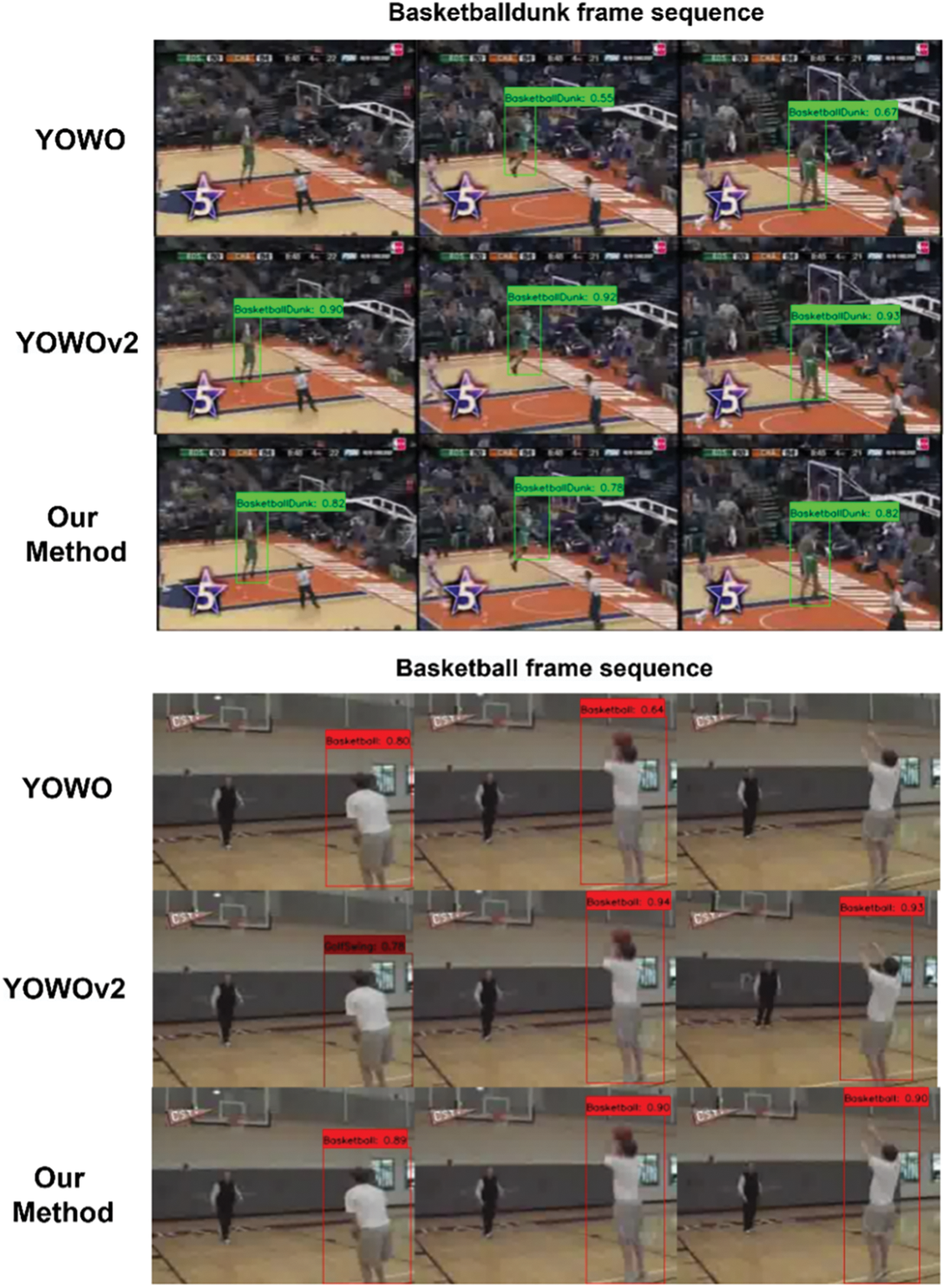
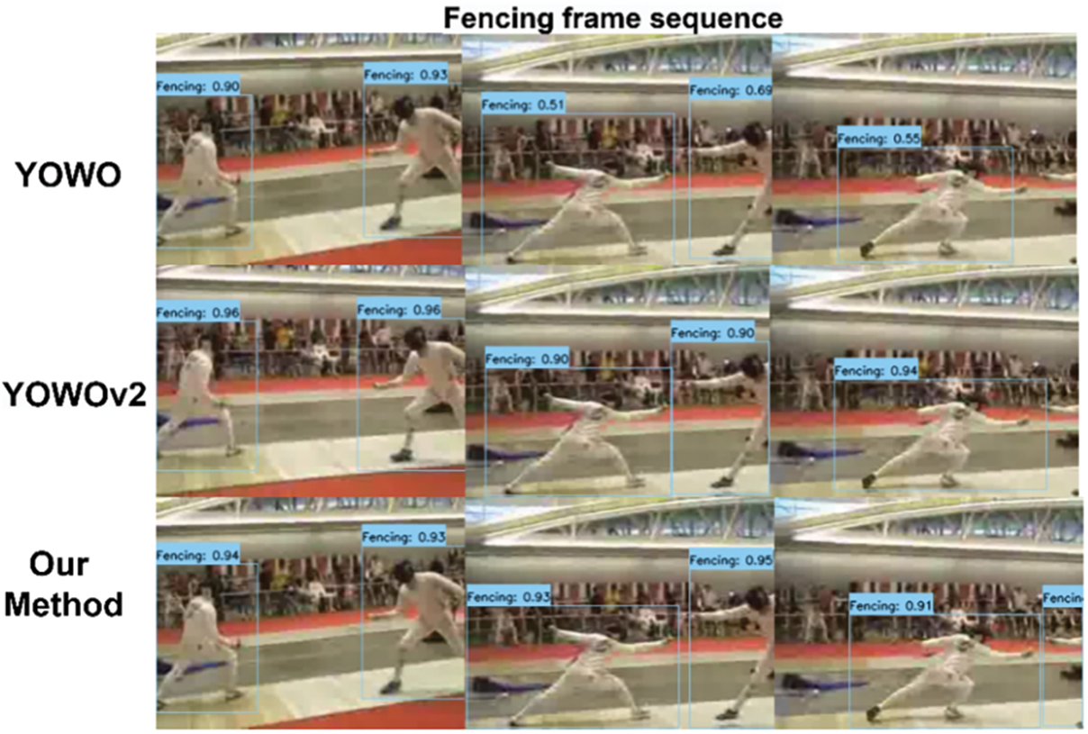
Figure 6: Comparison of continuous frame visualization results for STAD

Fig. 7 is a visualization comparison of predicted object locations in STAD for the Basketball, Biking, LongJump, SalasSpin, and IceDancing actions from the UCF101-24 dataset using the YOWO, YOWOv2 and ACSF-ED algorithms (without applying maximum threshold). The black boxes represent GT objects, while the green boxes represent predicted objects. The first row displays the position prediction results of behavior objects by YOWO, while the following rows show the position prediction results by YOWOv2 and ACSF-ED. It can be observed that when ACSF-ED performs bounding box predictions for the mentioned five behavior objects, more predicted boxes tend to aggregate near the GT objects, and these predicted boxes are closer to the GT annotations themselves. For example, in the LongJump scenario in Fig. 7, our method enables multiple predicted boxes (green) to concentrate more on the long-jumper object. On the other hand, the YOWO, due to its anchor-based approach, produces predicted boxes of more scattered and varied sizes. The YOWOv2 employs an anchor-free approach, leading to a noticeable improvement in the prediction box clustering compared to YOWO. However, in comparison to ACSF-ED, its clustering is still relatively loose. This phenomenon can be attributed to the fact that our proposed ACSF-ED does not rely on setting fixed anchor boxes of different sizes at the same position for prediction. Furthermore, ACSF-ED is trained using a multi-constraint loss function. Among these constraints, the one-to-many loss function is particularly effective in constraining unmatched candidates, resulting in a more concentrated distribution of predicted bounding boxes that closely approximate the GT.

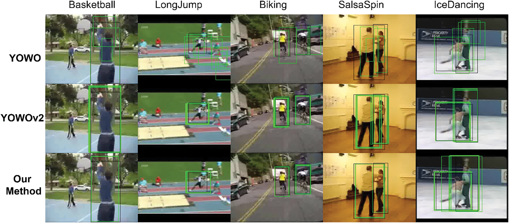
Figure 7: Comparison of visualizations for predicted bounding boxes in object regression (black box represents GT, green box represents predicted box)

4.4.2 Quantitative Performance Comparison

To objectively and fairly evaluate the performance superiority of our proposed algorithm, the ACSF-ED algorithm was compared with other excellent algorithms such as T-CNN [9], Action Tubelet Detector (ACT) [10], Multiple Path Search (MPS) [53], SAMOC [14], STEP [12], TubeR [7], YOWO [8], YOWOv2 [24], YOWOv3 [25] on the UCF101-24 dataset and JHMDB-21 dataset. This comparison was based on quantitative metrics including computational complexity (FLOPS), model parameters (Param), Frame-mAP (at an IoU threshold of 0.5), and Video-mAP (at an IoU threshold of 0.1), as shown in Table 1.

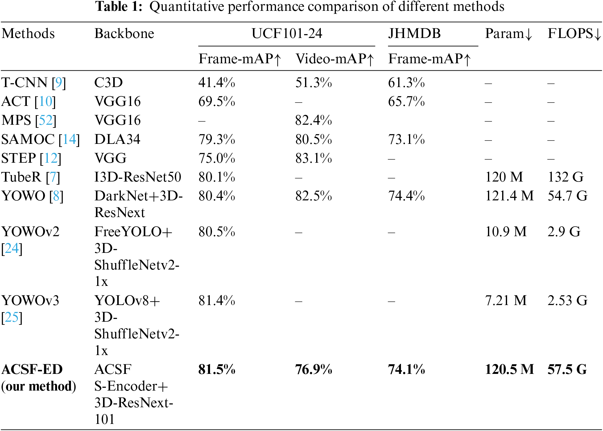
In terms of precision metrics comparison, our method ACSF-ED achieves a Frame-mAP detection result of 81.52% in the UCF101-24 dataset at an IoU threshold of 0.5. Among the algorithms listed above, most of those with performance below 80% are Clip-Level methods. These methods, as they predict action categories for the given tubelets, exhibit relatively lower performance on Frame-mAP evaluations. ACSF-ED outperforms these Clip-Level methods. YOWO and TubeR performed well, with scores of 80.4% and 80.1%, respectively on this metric. Our method surpassed YOWO by 1.1% and showed a 1.4% improvement compared to TubeR. Recently, variants of the YOWO series, YOWOv2, and YOWOv3, have achieved results of 80.5% and 81.4% on this metric. Our ACSF-ED still outperforms lightweight YOWOv2 by 1% and is 0.1% higher than the YOWOv3. Clearly, ACSF-ED demonstrates excellent performance on the UCF101-24 dataset in terms of Frame-mAP. In addition, ACSF-ED also achieved the Video-mAP metric on this dataset. It attained performance of 76.9% at an IoU threshold of 0.1, surpassing T-CNN by 15.6% and showing a 6% difference compared to Clip-Level methods like SAMOC. Overall, ACSF-ED demonstrates good performance relative to these comparisons. On another dataset JHMDB, the ACSF-ED algorithm also achieved a suboptimal result in terms of Frame-mAP among the compared algorithms. It obtained a detection result of 74.1% at an IoU threshold of 0.5, surpassing SAMOC by 1%. Its detection result is comparable to YOWO, differing by only 0.3%. This indicates that the ACSF-ED algorithm demonstrates excellent results on both the UCF101-24 and JHMDB datasets (particularly in terms of Frame-mAP), showcasing its consistently superior performance across different datasets. The reason why the algorithms mentioned perform well is closely related to our proposed ACCFM and its decoder. Through the ACCFM module, ACSF-ED can extract richer multi-scale feature information compared to YOWO, which uses a single-scale feature extraction method. The adaptive structure can also progressively propagate attention information from higher-level features to other scale features. This approach reduces losses in cross-scale propagation and fusion compared to the traditional pyramid structure used in the YOWOv2 method. Processing and detecting multi-scale information can significantly enhance detection capabilities across various scales. Additionally, compared to YOWO’s direct prediction after feature extraction, the decoder structure of ACSF-ED can provide a better understanding of the extracted features.

In terms of model complexity (specifically computational complexity FLOPS and model parameters Param), our ACSF-ED algorithm demonstrates a considerable reduction in computational complexity when compared to the pure 3D transformer method TubeR. Specifically, we observe a reduction of approximately 75 GFLOPS, while the number of model parameters is reduced by 0.9 M compared to YOWO. This reduction can be primarily attributed to the simplified Encoder-Decoder structure employed in ACSF-ED. In ACSF-ED, the encoder focuses solely on attention mechanism calculation for deep semantics, and the detection heads in the decoder are designed to be shared. However, compared to the latest lightweight versions of YOWOv2 and YOWOv3, our method still has a higher computational and parameter complexity. This is attributed to the lightweight 3D backbones employed in those two algorithms. This is an area where we can draw inspiration for future improvements and enhancements.

4.4.3 Comparison of the Frame AP in Each Action Class

To visually demonstrate the detection performance of ACSF-ED for each action class, this method was compared with the YOWO model on the UCF101-24 dataset in terms of average precision (AP) accuracy for each action class at the frame level. This comparison can be seen in Fig. 8. The UCF101-24 dataset comprises 24 action classes, hence the x-axis in Fig. 8 represents the class numbers, while the y-axis denotes the AP accuracy scores. As illustrated in Fig. 8, our model exhibits significantly improved AP for 13 action classes compared to YOWO, such as LongJump, Surfing, and BasketballDunk. For these particular classes, ACSF-ED achieved AP values of 62.89%, 91.32%, and 76.42%, respectively. Relative to the values obtained by YOWO, ACSF-ED shows enhancements of 5%, 5%, and 10% in AP for these classes. Furthermore, the detection performance for 7 additional action classes is comparable between ACSF-ED and YOWO. It is evident that our method demonstrates strong recognition and understanding capabilities across various action categories.

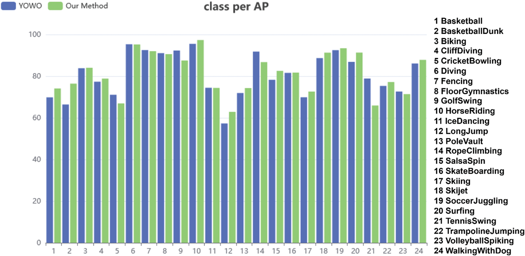
Figure 8: Comparison of the frame AP for each action class

4.5 Ablation Experiments

4.5.1 ACCFM Module Ablation Experiment

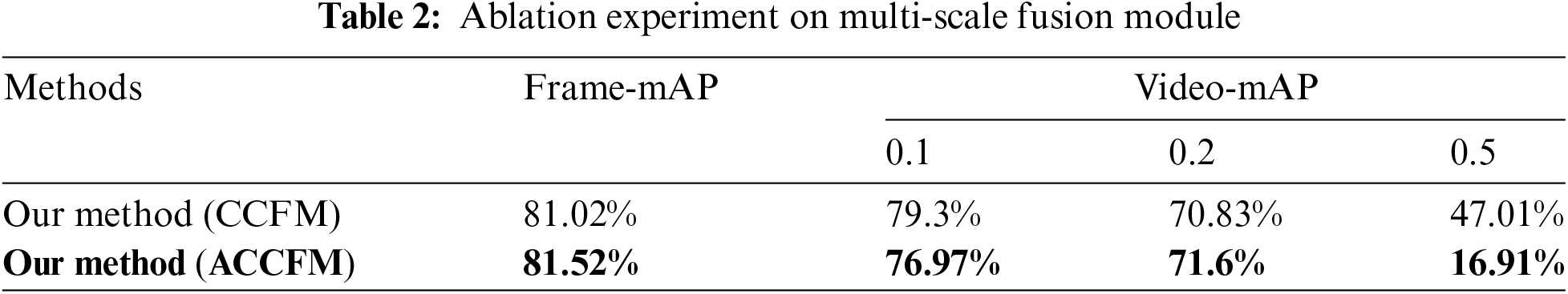
ACCFM plays a vital role in our methodology. To demonstrate its effectiveness, ablation experiments were conducted on the UCF101-24 dataset, using the main framework described in the paper, to validate both CCFM [42] and ACCFM. Analysis of Table 2 reveals that integration of the ACCFM module for cross-scale fusion in the main framework enables the entire model to achieve a detection performance metric of 81.52% in Frame-mAP with an IoU of 0.5. Compared to models that utilize the traditional feature pyramid fusion network CCFM as the fusion module, this approach effectively enhances detection accuracy by 0.5%. Moreover, the model employing the ACCFM module achieves Video-mAP metrics of 76.97% and 71.6% at IoU thresholds of 0.1 and 0.2, respectively, surpassing the model utilizing CCFM by 0.6% and 0.8%. These findings indicate that the adaptive cross-scale fusion module can significantly enhance the overall detection performance.

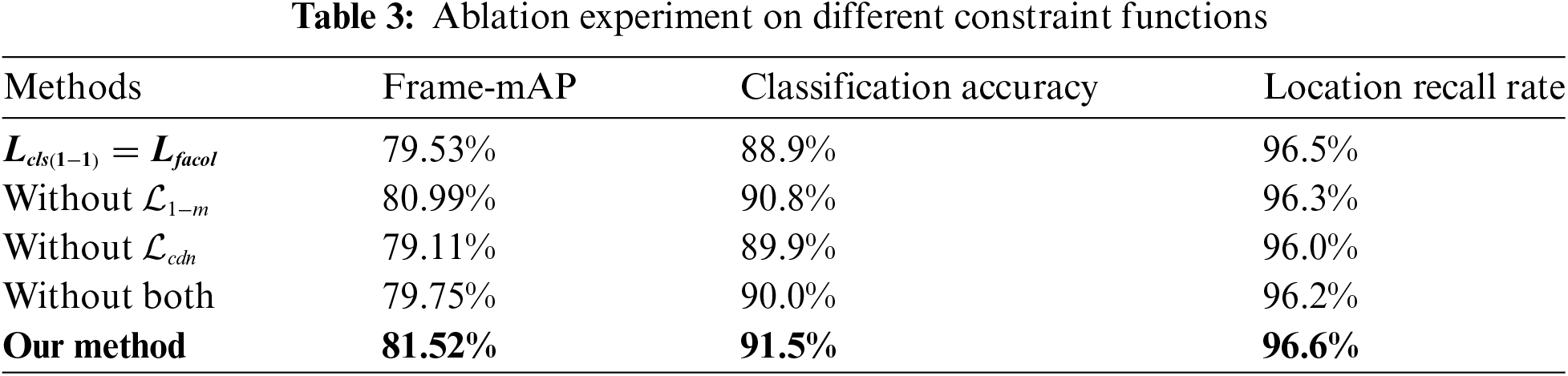
4.5.2 Multi-Constraint Loss Function Experiment

The multi-constraint function proposed for the Shared-Header Decoder plays an effective role in constraining the overall learning and understanding of the ACSF-ED model. In this context, a series of ablation experiments on the loss function of the main framework on the UCF101-24 dataset were conducted to showcase the predictive outcomes of the model under different constraint conditions, thereby demonstrating the advantages of our multi-constraint function. The experimental results in Table 3 illustrate that under the conditions of multiple constraint function, our model achieves the best classification and regression results: with a classification accuracy of 91.5%, a location recall rate of 96.6%, and a Frame-mAP (IoU = 0.5) of 81.52%. When the classification loss in the model’s one-to-one loss function is changed from VFL to Binary CrossEntropy (BCE), as indicated in the second row, the model’s Frame-map decreases by 1.99%, and the classification accuracy also drops by 2.6%. This indicates that without using the VFL loss function with IoU scores, some detections with high IoU but low scores will be filtered out, leading to a noticeable decrease in classification recall. When the model’s loss function lacks the one-to-many function, as indicated in the third row, the constraints of multiple candidate boxes being discarded result in the candidate boxes being solely subject to one-to-one constraints. Consequently, some regression boxes do not accurately localize to the ground truth, leading to the model’s location recall rate decreasing by 0.3%, classification accuracy decreasing by 0.7%, and the overall Frame-mAP decreasing by 0.53%. When the model’s loss function lacks the CDN constraint (i.e., removing the CDN module step), as shown in the fourth row, it means that the model does not learn the features of non-behavioral objects through additional denoising knowledge during training. This results in a decrease of 0.4% in location recall rate, 1.6% in classification accuracy, and 1.75% in Frame-mAP, leading to an overall performance decrease in Frame-mAP of 1.75%. When both the one-to-many constraint and the CDN constraint are not considered, the model’s location recall rate, classification accuracy, and Frame-mAP values are only 96.2%, 90.00%, and 79.75%, respectively, representing decreases of 0.4%, 1.5%, and 1.77%. This indicates that the model can enhance detection performance by learning and understanding on the training set through the multi-constraint loss function.

5  Conclusion

In this paper, we propose the end-to-end ACSF-ED network for the classification and localization of objects’ actions in videos. The ACCFM aids in extracting high-quality spatial information at each scale through adaptive cross-scale fusion, facilitating the fusion of spatial and spatio-temporal information for subsequent modules to learn and understand. Additionally, owing to the end-to-end network design, we introduce a multi-constraint loss function to jointly constrain the training of the entire model. This optimization not only enhances the selection results of the encoder but also improves the understanding and learning of the selection results by the decoder. Compared to some advanced spatio-temporal action detection algorithms, ACSF-ED achieves superior performance in the Frame-mAP metric. As a result, the ACSF-ED network can be applied to scenarios such as behavior detection in CCTV videos in public places, including detecting theft, fights, assaults, and armed robberies. It can also be used in production environments for detecting violations, or in identifying dangerous driving behaviors of motor vehicle drivers. Improved detection capabilities can enable people to confidently rely on automated technical surveillance rather than manual video monitoring in these scenarios. The practical applications of STAD can assist individuals, enhance work efficiency, and simplify daily life.

ACSF-ED demonstrates good performance on the UCF101-24 and JHMDB datasets, particularly in distinguishing individual action movements. However, the model’s detection capability for segments containing multiple different actions, such as in AVA, requires further investigation. Additionally, there is room for improvement in ACSF-ED. The 3D backbone in ACSF-ED bears the heaviest computational burden within the entire network architecture, consuming significant memory and computation resources, making the spatio-temporal feature extractor network somewhat bulky. To deploy detection on edge devices or achieve more efficient real-time performance, a more compact network design is necessary for the spatio-temporal feature extractor. Future works will focus on researching lighter spatio-temporal detection networks, as lightweight network holds greater practical value for real-world applications.

Acknowledgement: The authors would like to thank the Center for Research in Computer Vision at the University of Central Florida and the MPI for Intelligent Systems set used in this study.

Funding Statement: The financial support for this work was supported by Key Lab of Intelligent and Green Flexographic Printing under Grant ZBKT202301.

Author Contributions: All authors made significant contributions to this work. The contribution to the paper as follows: study conception and design: Zehua Gu, Wenju Wang; analysis and interpretation: Zehua Gu, Bang Tang; analysis tools: Sen Wang, Jianfei Hao. All authors reviewed the results and approved the final version of the manuscript.

Availability of Data and Materials: Our source code will available at https://github.com/Gu-ZH-cn/ACSF-ED (accessed on 05 November 2024). The UCF101-24 and JHMDB-21 data used in this study were obtained from public domain and are available online at https://www.crcv.ucf.edu/research/data-sets/ucf101/ (accessed on 05 November 2024) and http://jhmdb.is.tue.mpg.de/dataset (accessed on 05 November 2024).

Ethics Approval: Not applicable.

Conflicts of Interest: The authors declare no conflicts of interest to report regarding the present study.

References

1. W. S. Kim and K. K. Kim, “Abnormal detection of worker by interaction analysis of accident-causing objects,” in 32nd IEEE Int. Conf. Robot Human Interact. Commun., RO-MAN 2023, Busan, Republic of Korea, IEEE Computer Society, Aug. 28–31, 2023, pp. 884–889. doi: 10.1109/RO-MAN57019.2023.10309578. [Google Scholar] [CrossRef]

2. C. Yang, D. Chen, and Z. Xu, “Action recognition system for security monitoring,” in 2021 Int. Conf. Artif. Intell., Virtual Real. Visual., AIVRV 2021, Sanya, China, Academic Exchange Information Center (AEICNov. 19–21, 2021, vol. 12153. doi: 10.1117/12.2626689. [Google Scholar] [CrossRef]

3. M. Liang, X. Li, S. Onie, M. Larsen, and A. Sowmya, “Improved spatio-temporal action localization for surveillance videos,” in 2021 Int. Conf. Digital Image Comput.: Tech. Appl., DICTA 2021, Gold Coast, QLD, Australia, Nov. 29–Dec. 1, 2021, pp. 1–8. doi: 10.1109/DICTA52665.2021.9647106. [Google Scholar] [CrossRef]

4. M. A. S. Khan, M. J. B. Showmik, T. Ahmed, and A. F. M. S. Saif, “A constructive review on pedestrian action detection, recognition and prediction,” in 2nd Int. Conf. Comput. Adv. ICCA 2022, Dhaka, Bangladesh, Association for Computing Machinery, Mar. 10–12, 2022, pp. 367–376. doi: 10.1145/3542954.3543007. [Google Scholar] [CrossRef]

5. F. Ma, G. Xing, and Y. Liu, “Video-based driver action recognition via spatial-temporal and motion deep learning,” in 2023 Int. Joint Conf. Neural Netw., IJCNN 2023, Gold Coast, QLD, Australia, Jun. 18–23, 2023, pp. 1–9. doi: 10.1109/IJCNN54540.2023.10191918. [Google Scholar] [CrossRef]

6. C. Feichtenhofer, H. Fan, J. Malik, and K. He, “Slowfast networks for video recognition,” in 17th IEEE/CVF Int. Conf. Comput. Vis., ICCV 2019, Seoul, Republic of Korea, Institute of Electrical and Electronics Engineers Inc., Oct. 27–Nov. 2, 2019, pp. 6201–6210. doi: 10.1109/ICCV.2019.00630. [Google Scholar] [CrossRef]

7. J. Zhao et al., “TubeR: Tubelet transformer for video action detection,” in 2022 IEEE/CVF Conf. Comput. Vis. Pattern Recognit., CVPR 2022, New Orleans, LA, USA, IEEE Computer Society, Jun. 19–24, 2022, pp. 13588–13597. doi: 10.1109/CVPR52688.2022.01323. [Google Scholar] [CrossRef]

8. O. Kopuklu, X. Wei, and G. Rigoll, “You only watch once: A unified CNN architecture for real-time spatiotemporal action localization,” 2019, arXiv:1911.06644. [Google Scholar]

9. R. Hou, C. Chen, and M. Shah, “Tube convolutional neural network (T-CNN) for action detection in videos,” in 16th IEEE Int. Conf. Comput. Vis., ICCV 2017, Venice, Italy, Institute of Electrical and Electronics Engineers Inc., Oct. 22–29, 2017, pp. 5823–5832. doi: 10.1109/ICCV.2017.620. [Google Scholar] [CrossRef]

10. V. Kalogeiton, P. Weinzaepfel, V. Ferrari, and C. Schmid, “Action tubelet detector for spatio-temporal action localization,” in 16th IEEE Int. Conf. Comput. Vis., ICCV 2017, Venice, Italy, Institute of Electrical and Electronics Engineers Inc., Oct. 22–29, 2017, pp. 4415–4423. doi: 10.1109/ICCV.2017.472. [Google Scholar] [CrossRef]

11. W. Liu et al., “SSD: Single shot multibox detector,” in 14th European Conf. Comput. Vis., ECCV 2016, Amsterdam, Netherlands, Springer Verlag, Oct. 8–16, 2016, pp. 21–37. doi: 10.1007/978-3-319-46448-0_2. [Google Scholar] [CrossRef]

12. X. Yang, X. Yang, M. -Y. Liu, F. Xiao, L. S. Davis and J. Kautz, “STEP: Spatio-temporal progressive learning for video action detection,” in 32nd IEEE/CVF Conf. Comput. Vis. Pattern Recognit., CVPR 2019, Long Beach, CA, USA, IEEE Computer Society, Jun. 16–20, 2019, pp. 264–272. doi: 10.1109/CVPR.2019.00035. [Google Scholar] [CrossRef]

13. Y. Li, Z. Wang, L. Wang, and G. Wu, “Actions as moving points,” in 16th Eur. Conf. Comput. Vis., ECCV 2020, Glasgow, UK, Springer Science and Business Media Deutschland GmbH, Aug. 23–28, 2020, pp. 68–84. doi: 10.1007/978-3-030-58517-4_5. [Google Scholar] [CrossRef]

14. X. Ma, Z. Luo, X. Zhang, Q. Liao, X. Shen and M. Wang, “Spatio-temporal action detector with self-attention,” in 2021 Int. Jt. Conf. Neural Netw., IJCNN 2021, Shenzhen, China, Jul. 18–22, 2021, pp. 1–8. doi: 10.1109/IJCNN52387.2021.9533300. [Google Scholar] [CrossRef]

15. K. Duarte, Y. S. Rawat, and M. Shah, “VideocapsuleNet: A simplified network for action detection,” in 32nd Conf. Neural Inf. Process. Syst., NeurIPS 2018, Montreal, QC, Canada, Neural Information Processing Systems Foundation, Dec. 2–8, 2018, pp. 7610–7619. [Google Scholar]

16. L. Song, S. Zhang, G. Yu, and H. Sun, “TACNet: Transition-aware context network for spatio-temporal action detection,” in 32nd IEEE/CVF Conf. Comput. Vis. Pattern Recognit., CVPR 2019, Long Beach, CA, USA, IEEE Computer Society, Jun. 16–20, 2019, pp. 11979–11987. doi: 10.1109/CVPR.2019.01226. [Google Scholar] [CrossRef]

17. G. Gkioxari and J. Malik, “Finding action tubes,” in IEEE Conf. Comput. Vis. Pattern Recognit., CVPR 2015, Boston, MA, USA, IEEE Computer Society, Jun. 7–12, 2015, pp. 759–768. doi: 10.1109/CVPR.2015.7298676. [Google Scholar] [CrossRef]

18. S. Saha, G. Singh, M. Sapienza, P. H. S. Torr, and F. Cuzzolin, “Deep learning for detecting multiple space-time action tubes in videos,” in 27th British Mach. Vis. Conf., BMVC 2016, York, UK, Sep. 19–22, 2016, pp. 58.1–58.13. doi: 10.5244/C.30.58. [Google Scholar] [CrossRef]

19. X. Peng and C. Schmid, “Multi-region two-stream R-CNN for action detection,” in 21st ACM Conf. Comput. Commun. Secur., CCS 2014, Scottsdale, AZ, USA, 2016, Springer Verlag, Nov. 3–7, 2014, pp. 744–759. doi: 10.1007/978-3-319-46493-0_45. [Google Scholar] [CrossRef]

20. Z. Yang, J. Gao, and R. Nevatia, “Spatio-temporal action detection with cascade proposal and location anticipation,” in 28th British Mach. Vis. Conf., BMVC 2017, London, UK, Sep. 4–7, 2017. doi: 10.48550/arXiv.2308.01618. [Google Scholar] [CrossRef]

21. C. Gu et al., “AVA: A video dataset of spatio-temporally localized atomic visual actions,” in 31st Meet. IEEE/CVF Conf. Comput. Vis. Pattern Recognit., CVPR 2018, Salt Lake City, UT, USA, IEEE Computer Society, Jun. 18–22, 2018, pp. 6047–6056. doi: 10.1109/CVPR.2018.00633. [Google Scholar] [CrossRef]

22. C. Feichtenhofer, “Expanding architectures for efficient video recognition,” in 2020 IEEE/CVF Conf. Comput. Vis. Pattern Recognit., CVPR 2020, Seattle, WA, USA, IEEE Computer Society, Jun. 14–19, 2020, pp. 200–210. doi: 10.1109/CVPR42600.2020.00028. [Google Scholar] [CrossRef]

23. S. Chen et al., “Watch only once: An end-to-end video action detection framework,” in 18th IEEE/CVF Int. Conf. Comput. Vis., ICCV 2021, Montreal, QC, Canada, Institute of Electrical and Electronics Engineers Inc., Oct. 11–Oct. 17, 2021, pp. 8158–8167. doi: 10.1109/ICCV48922.2021.00807. [Google Scholar] [CrossRef]

24. J. Yang and K. Dai, “YOWOv2: A stronger yet efficient multi-level detection framework for real-time spatio-temporal action detection,” 2023, arXiv:2302.06848. [Google Scholar]

25. N. D. D. Manh, D. V. Hang, J. C. Wang, and B. D. Nhan, “YOWOv3: An efficient and generalized framework for human action detection and recognition,” 2024, arXiv:2408.02623. [Google Scholar]

26. C. Szegedy et al., “Going deeper with convolutions,” in IEEE Conf. Comput. Vis. Pattern Recognit., CVPR 2015, Boston, MA, USA, IEEE Computer Society, Jun. 7–12, 2015, pp. 1–9. doi: 10.1109/CVPR.2015.7298594. [Google Scholar] [CrossRef]

27. K. He, X. Zhang, S. Ren, and J. Sun, “Spatial pyramid pooling in deep convolutional networks for visual recognition,” IEEE Trans. Pattern Anal. Mach. Intell., vol. 37, no. 9, pp. 1904–1916, 2015. doi: 10.1109/TPAMI.2015.2389824. [Google Scholar] [PubMed] [CrossRef]

28. H. Zhao, J. Shi, X. Qi, X. Wang, and J. Jia, “Pyramid scene parsing network,” in 30th IEEE Conf. Comput. Vis. Pattern Recognit., CVPR 2017, Honolulu, HI, USA, Jul. 21–26, 2017, pp. 6230–6239. doi: 10.1109/CVPR.2017.660. [Google Scholar] [CrossRef]

29. T. -Y. Lin, P. Dollar, R. Girshick, K. He, B. Hariharan and S. Belongie, “Feature pyramid networks for object detection,” in 30th IEEE Conf. Comput. Vis. Pattern Recognit., CVPR 2017, Honolulu, HI, USA, Jul. 21–26, 2017, pp. 936–944. doi: 10.1109/CVPR.2017.106. [Google Scholar] [CrossRef]

30. S. Liu, D. Huang, and Y. Wang, “Learning spatial fusion for single-shot object detection,” 2019, arXiv:1911.09516. [Google Scholar]

31. R. Girshick, J. Donahue, T. Darrell, and J. Malik, “Rich feature hierarchies for accurate object detection and semantic segmentation,” in 27th IEEE Conf. Comput. Vis. Pattern Recognit., CVPR 2014, Columbus, OH, USA, IEEE Computer Society, Jun. 23–28, 2014, pp. 580–587. doi: 10.1109/CVPR.2014.81. [Google Scholar] [CrossRef]

32. Z. Tian, C. Shen, H. Chen, and T. He, “FCOS: Fully convolutional one-stage object detection,” in 17th IEEE/CVF Int. Conf. Comput. Vis., ICCV 2019, Seoul, Republic of Korea, Institute of Electrical and Electronics Engineers Inc., Oct. 27–Nov. 2, 2019, pp. 9626–9635. doi: 10.1109/ICCV.2019.00972. [Google Scholar] [CrossRef]

33. J. Redmon and A. Farhadi, “YOLOv3: An incremental improvement,” 2018, arXiv:1804.02767. [Google Scholar]

34. A. Bochkovskiy, C. -Y. Wang, and H. -Y. M. Liao, “YOLOv4: Optimal speed and accuracy of object detection,” 2020, arXiv:2004.10934. [Google Scholar]

35. C. -Y. Wang, A. Bochkovskiy, and H. -Y. M. Liao, “YOLOv7: Trainable bag-of-freebies sets new state-of-the-art for real-time object detectors,” in 2023 IEEE/CVF Conf. Comput. Vis. Pattern Recognit. (CVPR), Vancouver, BC, Canada, 2023, pp. 7464–7475. doi: 10.1109/CVPR52729.2023.00721. [Google Scholar] [CrossRef]

36. C. Li et al., “YOLOv6 v3.0: A full-scale reloading,” 2023, arXiv:2301.05586. [Google Scholar]

37. Z. Ge, S. Liu, F. Wang, Z. Li, and J. Sun, “YOLOX: Exceeding YOLO series in 2021,” 2021, arXiv:2107.08430. [Google Scholar]

38. A. Vaswani et al., “Attention is all you need,” in 31st Annual Conf. Neural Inf. Process. Syst., NIPS 2017, Long Beach, CA, USA, Neural Information Processing Systems Foundation, Dec. 4–9, 2017, pp. 5999–6009. doi: 10.48550/arXiv.1706.03762. [Google Scholar] [CrossRef]

39. N. Carion, F. Massa, G. Synnaeve, N. Usunier, A. Kirillov and S. Zagoruyko, “End-to-end object detection with transformers,” in Comput. Vis.-ECCV 2020: 16th Eur. Conf., 2020, pp. 213–229. doi: 10.1007/978-3-030-58452-8_13. [Google Scholar] [CrossRef]

40. S. Liu et al., “Dynamic anchor boxes are better queries for detr,” in 10th Int. Conf. Learn. Representations, ICLR 2022, Apr. 25–29, 2022. [Google Scholar]

41. F. Li, H. Zhang, S. Liu, J. Guo, L. M. Ni and L. Zhang, “DN-DETR: Accelerate DETR training by introducing query DeNoising,” IEEE Trans. Pattern Anal. Mach. Intell., vol. 46, no. 4, pp. 2239–2251, 2024. doi: 10.1109/TPAMI.2023.3335410. [Google Scholar] [PubMed] [CrossRef]

42. Y. Zhao et al., “DETRs beat YOLOs on real-time object detection,” in 2024 IEEE/CVF Conf. Comput. Vis. Pattern Recognit. (CVPR), Seattle, WA, USA, 2024, pp. 16965–16974. doi: 10.1109/CVPR52733.2024.01605. [Google Scholar] [CrossRef]

43. N. D. S. Battula, H. R. Kambhampaty, Y. Vijayalata, and R. N. Ashlin Deepa, “Deep-learning residual network based image analysis for an efficient two-stage recognition of neurological disorders,” in 2nd Int. Conf. Innov. Technol., INOCON 2023, Bangalore, India, Institute of Electrical and Electronics Engineers Inc., Mar. 3–5, 2023. doi: 10.1109/INOCON57975.2023.10101037. [Google Scholar] [CrossRef]

44. J. Lin, X. Mao, Y. Chen, L. Xu, Y. He and H. Xue, “D2ETR: Decoder-only DETR with computationally efficient cross-scale attention,” 2022, arXiv:2203.00860. [Google Scholar]

45. S. Xie, R. Girshick, P. Dollar, Z. Tu, and K. He, “Aggregated residual transformations for deep neural networks,” in 30th IEEE Conf. Comput. Vis. Pattern Recognit., CVPR 2017, Honolulu, HI, USA, Institute of Electrical and Electronics Engineers Inc., Jul. 21–26, 2017, pp. 5987–5995. doi: 10.1109/CVPR.2017.634. [Google Scholar] [CrossRef]

46. X. Ding, X. Zhang, N. Ma, J. Han, G. Ding and J. Sun, “RepVGG: Making VGG-style ConvNets great again,” in 2021 IEEE/CVF Conf. Comput. Vis. Pattern Recognit., CVPR 2021, Nashville, TN, USA, IEEE Computer Society, Jun. 19–25, 2021, pp. 13728–13737. doi: 10.1109/CVPR46437.2021.01352. [Google Scholar] [CrossRef]

47. J. Fu et al., “Dual attention network for scene segmentation,” in 32nd IEEE/CVF Conf. Comput. Vis. Pattern Recognit., CVPR 2019, Long Beach, CA, USA, IEEE Computer Society, Jun. 16–20, 2019, pp. 3141–3149. doi: 10.1109/CVPR.2019.00326. [Google Scholar] [CrossRef]

48. Anonymous, “DINO: DETR with improved denoising anchor boxes for end-to-end object detection,” in 11th Int. Conf. Learn. Representations, ICLR 2023, Kigali, Rwanda, Google Research, May 1–5, 2023. doi: 10.48550/arXiv.2203.03605. [Google Scholar] [CrossRef]

49. H. Lin, X. Cheng, X. Wu, and D. Shen, “CAT: Cross attention in vision transformer,” in 2022 IEEE Int. Conf. Multimed. Expo, ICME 2022, Taipei, Taiwan, Jul. 18–22, 2022. doi: 10.1109/TCSVT.2018.2887283. [Google Scholar] [CrossRef]

50. K. Soomro, A. Zamir, and M. J. A. Shah, “UCF101: A dataset of 101 human actions classes from videos in the wild,” 2012, arXiv:1212.0402. [Google Scholar]

51. H. Jhuang, J. Gall, S. Zuffi, C. Schmid, and M. J. Black, “Towards understanding action recognition,” in 2013 14th IEEE Int. Conf. Comput. Vis., ICCV 2013, Sydney, NSW, Australia, Institute of Electrical and Electronics Engineers Inc., Dec. 1–8, 2013, pp. 3192–3199. doi: 10.1109/ICCV.2013.396. [Google Scholar] [CrossRef]

52. M. Everingham, L. Van Gool, C. K. I. Williams, J. Winn, and A. Zisserman, “The pascal visual object classes (VOC) challenge,” Int. J. Comput. Vis., vol. 88, no. 2, pp. 303–338, 2010. doi: 10.1007/s11263-009-0275-4. [Google Scholar] [CrossRef]

53. E. H. P. Alwando, Y. -T. Chen, and W. -H. Fang, “CNN-based multiple path search for action tube detection in videos,” IEEE Trans. Circuits Syst. Video Technol., vol. 30, no. 1, pp. 104–116, 2020. doi: 10.1109/TCSVT.2018.2887283. [Google Scholar] [CrossRef]