Side-Scan Sonar Image Detection of Shipwrecks Based on CSC-YOLO Algorithm

1  Introduction

Currently, marine activities are increasingly frequent, and precise underwater object detection and identification are crucial for many economic and military activities, forming a core part of the strategy to build a maritime power [1,2]. Particularly, underwater shipwreck identification technology, as one of the important techniques in the field of marine surveying, plays a significant role in underwater cultural relic archaeology, detection and rescue of maritime shipwrecks, and the inspection of riverine obstacles [3–7], directly affecting the progress and effectiveness of these detection tasks. side-scan sonar, as an acoustic detection device, operates under low visibility conditions and is characterized by long range and high efficiency. It has become one of the technical means for countries to detect marine resources and military objects, employing its advantages of low cost and high resolution to mainly detect underwater objects like shipwrecks, torpedoes, aircraft debris, schools of fish, and more [8–11].

Object detection in side-scan sonar images typically relies on manual interpretation, which is a process fraught with many challenges: low operational efficiency, susceptibility to subjective influences, and various uncertain interference factors. Even more deadly is that in some cases, such as the underwater automatic mobile platform as a sonar carrier, manual interpretation is not allowed. To overcome these difficulties, the academic community has actively explored new methods and technologies for automatic object detection in side-scan sonar images in recent years [12,13]. Specifically, these methods can be divided into the traditional methods and the methods based on deep learning. The study on the methods based on deep learning is a hot topic in recent years, and they are divided into one-stage and two-stage object detection algorithms. Representative algorithms include R-CNN [14], Faster R-CNN [15], DETR [16], and the YOLO series [17]. Currently, the existing research on object detection in side-scan sonar images based on deep learning methods is mainly found in References [18–24]. Reference [18] applied R-CNN to the detection of categories such as soil, sand, and rock, finding that R-CNN performs better than traditional methods for detecting sonar images. Reference [19] was the first to apply the Faster R-CNN algorithm for side-scan sonar image detection, achieving high detection precision. However, despite its superiority over R-CNN, the detection time is too long to meet the real-time requirements for maritime search and rescue. Reference [20] applied the YOLO algorithm to object detection in forward-looking sonar images. It found that although YOLO improved detection speed compared to Faster R-CNN, the detection precision was not ideal. Reference [21] utilized the YOLOv3 algorithm model for underwater object detection in sonar images. The authors enhanced detection precision through data augmentation; however, they did not implement any internal model improvements, resulting in unchanged detection speed. Reference [22] proposed a sonar image object detection algorithm based on YOLOv5, named DETR-YOLO. It is designed for detecting underwater shipwreck objects. However, due to the large size of the DETR model, although the DETR-YOLO model improved detection precision, its detection speed decreased as a result. Reference [23] reorganized the YOLOv7 network and added a small object detection layer, which improved detection precision, but the increase in detection layers led to higher model complexity. Reference [24] made improvements to YOLOv5 by incorporating the CBAM [25] attention mechanism. In comparative experiments, the proposed model achieved the highest precision, but the model complexity also increased accordingly.

After analyzing the research on traditional methods and deep learning methods, it was found that in object detection studies involving side-scan sonar images, there is either a low detection precision or a slow detection speed, and no balanced solution has been proposed between these two issues. Moreover, no solutions have been proposed for the issue of insufficient sonar image data.

To address the aforementioned issues, this paper first employs offline data augmentation to increase the sample size of the dataset and utilizes online data augmentation combined with algorithms to tackle the small sample problem. Subsequently, this paper proposes a side-scan sonar shipwreck object detection method based on the CSC-YOLO (Context Guided Block, Shared Conv_Group Normalization Detection, Cross Stage Partial with 2 Partial Convolution-You Only Look Once) model, aimed at optimizing the model structure, reducing the number of parameters, and improving computational efficiency for accurate identification of shipwreck objects. The main improvements are as follows:

(1) Enhanced Feature Extraction Network: The traditional Convolution (Conv) module in the backbone is replaced with the Context Guided Block (CGB) module, which strengthens the model’s ability to capture key information in the images, thereby improving the precision of shipwreck detection.

(2) Constructing Lightweight Detection Head: To further enhance detection speed and precision, Group Normalization (GN) techniques are introduced and combined with convolution modules to form the Conv_GN module. This module is utilized as a shared convolution to design the SCGD detection head, which helps to simultaneously address the issues of low detection precision and slow detection response times.

(3) Improved Feature Fusion Network: To further reduce the model’s parameter count and computational load while increasing detection speed, we introduce the Partial Convolution (PConv) module to construct the Cross Stage Partial with 2 Partial Convolution (C2PC) module, which addresses the problem of slow detection response times.

The remainder of this paper is organized as follows: In Section 2, we introduce the source of the dataset and the methods employed to address the small sample problem. In Section 3, we provide a detailed description of the improvements made to CSC-YOLO, outlining the enhancements implemented in each module. In Section 4, we conduct various validation experiments to assess the performance of the CSC-YOLO model. In Section 5, we summarize the findings of this paper and engage in a discussion of their implications.

2  Dataset Preparation and Preprocessing

This chapter primarily discusses the source of the dataset, followed by methods for handling small sample datasets, including both offline and online data augmentation.

2.1 Dataset Source

The side-scan sonar images of shipwrecks are provided by the project “Deep Sea Shipwreck Sonar Image Segmentation Method Based on Interference-Resistant Two-Dimensional Attribute Histogram and Snake Model,” as well as collected from the Roboflow open dataset website [26], totaling 485 images, as shown in Fig. 1. The dataset was divided into training and validation sets in an 8:2 ratio, with the training set containing 388 shipwreck images and the validation set containing 97 shipwreck images.

Figure 1: Partial images of the dataset

2.2 Preprocessing for Small Sample Problems

Deep learning networks require a large amount of training data to effectively learn object features. However, a small dataset can lead to overfitting and poor generalization of the network. To address these issues, this paper implements data augmentation.

2.2.1 Offline Data Augmentation

Data Augmentation Based on HSV Domain Transformation: The HSV model uses Hue, Saturation, and Value to represent colors, reflecting human color perception intuitively, and is suitable for the analysis and processing of visual information. Due to the unique nature of side-scan sonar images, which are primarily generated based on the transducer’s emission and reception of sound waves, the displayed images vary in different scenarios. In deep sea environments, the sonar signal is heavily interfered with, often resulting in darker images. Additionally, based on factors such as model type, side-scan sonar images can be classified into grayscale and pseudocolor images.

Data Augmentation Based on Geometric Transformations: Expanding the dataset by altering image shapes can improve the generalization ability of the network model. As the transducer array scans the seabed, the state of shipwrecks is quite random. Therefore, applying random flips, rotations, and cropping can simulate various potential orientations of shipwrecks on the seabed.

Data Augmentation Based on Cutout Algorithm [27]: In object detection tasks, using random erasure can simulate scenarios with incomplete image information, such as issues caused by poor scanning quality of survey ships or damaged objects. This algorithm achieves this by randomly erasing small areas within images, which not only helps the model learn to recognize objects from incomplete images but also enhances the model’s capability to handle missing or poor-quality image data in practical applications.

As shown in Fig. 2, offline data augmentation was used to expand the side-scan sonar shipwreck images by four times, thereby significantly increasing the sample size of the shipwreck dataset. The method of splitting the dataset before augmentation was adopted to prevent multiple augmented images of the same original image from appearing in both the training and validation sets, which could reduce the model’s generalization ability. After data augmentation, the training set contains 1552 images, and the validation set contains 388 images.

Figure 2: Offline image data augmentation

From Fig. 3, it can be observed that Fig. 3a shows the positional statistics of the shipwreck objects within the entire image, indicating that most of the shipwreck objects are located in the central area of the image. Fig. 3b presents the statistical distribution of the height-to-width ratios of the shipwreck objects relative to the original image size, from which it can be seen that the height and width ratios of most shipwreck objects are less than 0.1, thus classifying them as small objects [28]. Since small objects are prone to being missed in detection, it can be concluded that detecting shipwrecks poses a significant challenge.

Figure 3: Distribution and size diagram of shipwreck objects. (a) The position distribution of the shipwreck objects in the image; (b) The size proportion of the shipwreck objects relative to the entire image

2.2.2 Online Data Augmentation

The Mosaic data augmentation method enriches the training data and improves model performance by randomly cropping and stitching four images into a new one [29]. Specifically, four side-scan sonar shipwreck images are randomly selected from the dataset, then randomly scaled, cropped, and cut before being stitched together in a random manner, as shown in Fig. 4. This method not only increases image diversity but also enhances batch processing efficiency because the composite image contains information from four images, simulating a larger batch size without increasing the physical batch size. This strategy effectively improves the model’s generalization ability with a limited dataset and optimizes the training process efficiency.

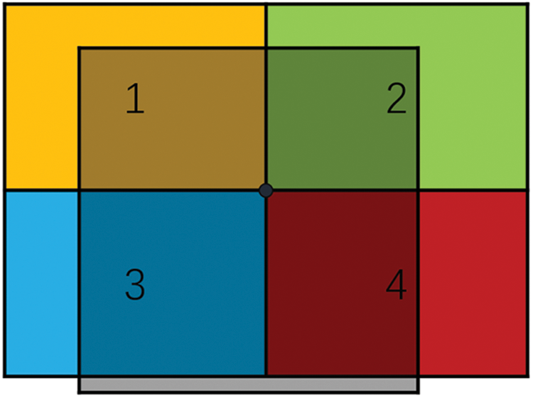
Figure 4: Diagram of the Mosaic algorithm

3  Improved YOLOv8 Model

This chapter selects the YOLOv8n [30] model for enhancement and provides a detailed description of the modifications made to the YOLOv8n model in this paper. Finally, the structure of the improved network model is presented.

3.1 YOLOv8 Network Improvement Methods

The YOLOv8n model, with its fewer parameters and fast computation speed, is particularly suitable for deployment on lightweight mobile devices. Therefore, this paper selects the YOLOv8n version from the YOLOv8 series as the baseline model and develops the CSC-YOLO network based on this for algorithm improvements.

3.1.1 Introduction of CGB Module

This paper introduces the CGB [31] module, as shown in Fig. 5. This module integrates four core components: a local feature extractor floc, a surrounding context extractor fsur, a joint feature extractor fjoi, and a global feature extractor fglo, mimicking the way human vision relies on contextual information to interpret scenes.

Figure 5: CGB module structure

In the initial stage, the module reduces the dimensionality of input features through 1 × 1 convolutions, simplifying subsequent processing steps and improving computational efficiency. The downscaled feature maps are then processed separately by the local feature extractor floc and the surrounding context extractor fsur, each focusing on the image’s local details and surrounding context information, thereby enhancing the module’s ability to analyze different regions of the image.

Next, the joint feature extractor fjoi merges the local and environmental context feature maps at the channel level, creating a fused feature representation. This representation combines local and contextual information, enhancing feature depth. The merged features are further enhanced through batch normalization and activation function adjustments, boosting feature expressiveness and the model’s robustness against interference.

Finally, the global feature extractor fglo deeply refines the fused feature representation by reducing dimensions and remapping to optimize features, eliminating unnecessary information and strengthening useful features. By integrating the extraction and refinement of local, contextual, and global features, the CGB module effectively leverages extensive contextual information within images, significantly enhancing feature representation and overall model performance.

In this paper, we extract the CGB module from CGNet [31] and improve it into a downsampling module to replace traditional convolutional modules, utilizing the CGB module in the feature extraction phase of deep convolutional neural networks. This approach aims to leverage a context-guided mechanism to enhance the network’s ability to learn and represent image features. By integrating the CGB module, we can enhance information integration, improving the overall performance and accuracy in handling complex visual tasks.

3.1.2 Design of SCGD Head

An ideal object detection head should meet the following criteria: efficiency, meaning it can accurately complete the detection task in a short time; precision, maintaining high recognition rates even with fast detection; and low miss rates, effectively identifying small objects to prevent missed detections. To achieve these performance metrics, this paper introduces the Group Normalization (GN) technique [32] and combines it with traditional Conv layers to form the Conv_GN module, as shown in Fig. 6. This module uses shared convolution, with group normalization independently standardizing within groups, effectively reducing parameters and computational load while enhancing detection speed and precision.

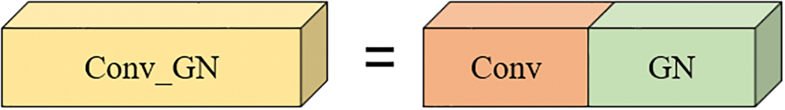
Figure 6: Conv_GN module structure

Based on the understanding of Reference [32], the GN calculation formula is summarized in Eqs. (1)–(3).

(1)

(2)

(3)

In the formula: i ∈ [1, G], C and G are the number of channels and groups, respectively, μG and σG are the mean and standard deviation of the input within the corresponding group, γ and β are learnable parameters used to adjust the normalized output yi. This setup allows the model to independently adjust the data distribution within each group, making network training more stable and efficient.

The paper posits that using GN significantly enhances the performance of detection heads in object localization and classification tasks. Based on this, the paper replaces the regular Conv modules in the detection head with Conv_GN modules to further improve precision in localization and classification. Initially, a single Conv_GN convolutional module is used to enhance detection performance. Subsequently, configuring two Conv_GN modules to perform shared convolution significantly reduces the model’s parameter count and computational demands. Additionally, to accommodate the varying object scales detected by different detection heads, a Scale layer is introduced on top of the shared convolution to appropriately scale features. The structure of the entire SCGD network is shown in Fig. 7.

Figure 7: SCGD head

3.1.3 Construction of C2PC Module

In practical applications of shipwreck detection, algorithm models often need to be deployed on platforms with limited computing capabilities. However, traditional algorithms frequently fail to meet the performance requirements of these low computing power platforms. Based on PConv technology [33], we designed a new structure, C2PC, to replace the C2f module in the Neck network. PConv is a form of convolution designed for high-speed inference, aimed at enhancing detection speed while reducing the model’s parameter count and computational load.

The core principle of PConv is to utilize the redundant parts of the input feature maps, applying convolution operations only on a subset of input channels to extract spatial features without altering the other channels. This approach significantly reduces the number of floating-point operations compared to traditional full convolution operations, thereby increasing computational efficiency, reducing the computational load, and lowering memory access frequency. By this means, PConv effectively captures spatial features while reducing computational and memory demands. The schematic diagram of PConv’s convolutional structure is shown in Fig. 8. This innovative structure makes the model more suitable for operation in resource-limited environments, especially in scenarios where rapid and efficient detection of shipwrecks is required.

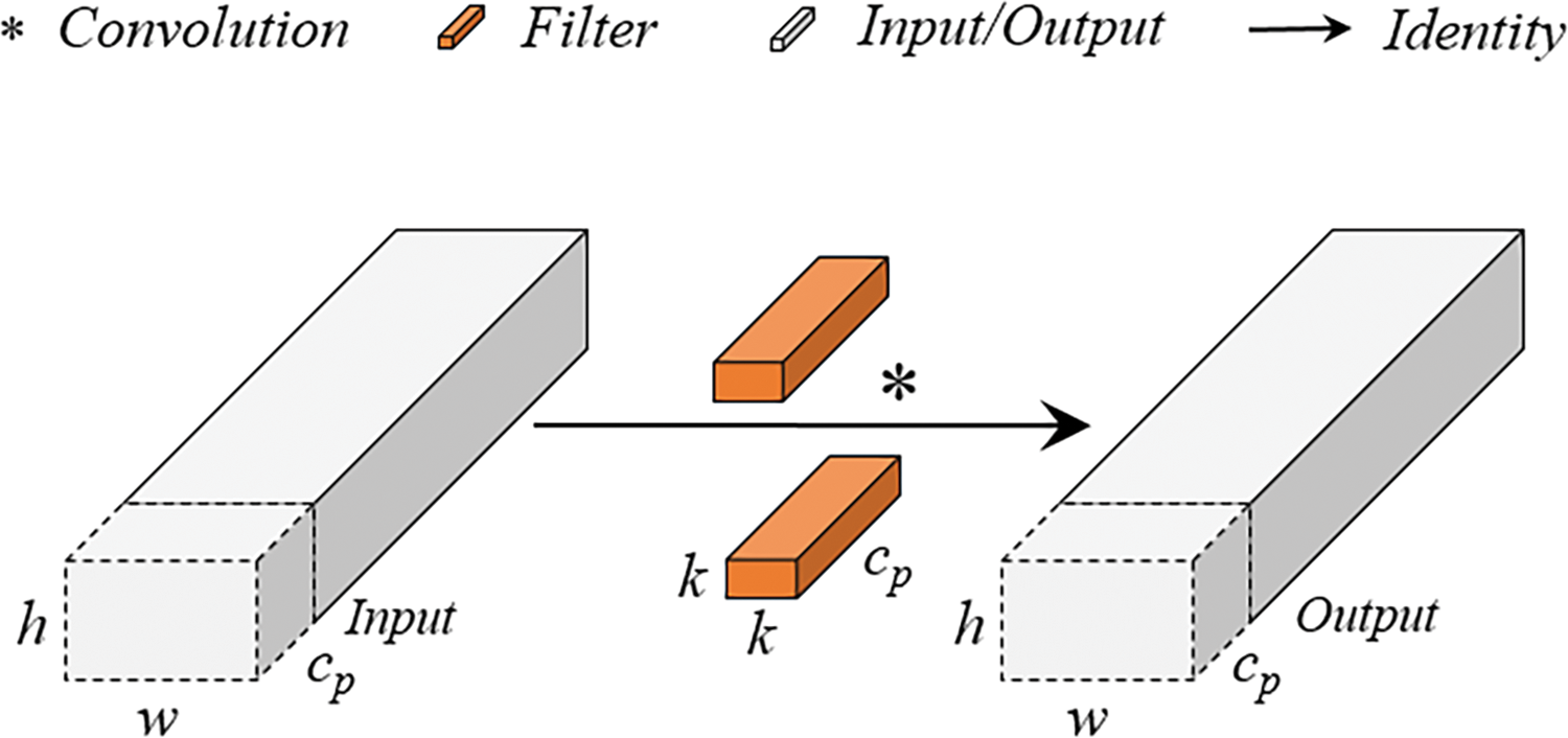
Figure 8: PConv structure

Using the PConv convolutional design module can reduce the model’s parameter count and computational load, minimize information loss, and enhance the model’s expressive capabilities. The formula for its calculated volume is shown in Eqs. (4) and (5).

(4)

(5)

In the formula: h and w are the height and width of the feature map; k is the size of the convolution kernel; cp is the number of channels participating in the convolution; r is the convolution participation rate, typically set at 1/4 in practical applications, meaning the computational cost of PConv is 1/16 that of a regular convolution; c is the number of input channels.

The memory access of PConv is calculated as shown in Eq. (6).

(6)

During the convolution process, memory usage is low, and the memory access required for PConv convolution is far less than that for standard Conv convolution. This paper utilizes PConv to design the C2PC module to replace the C2f module in the Neck network, as shown in Fig. 9. This allows for increased detection speed and further enhances detection precision. The introduction of PConv convolution effectively streamlines the network model structure while significantly saving computational resources and improving detection precision.

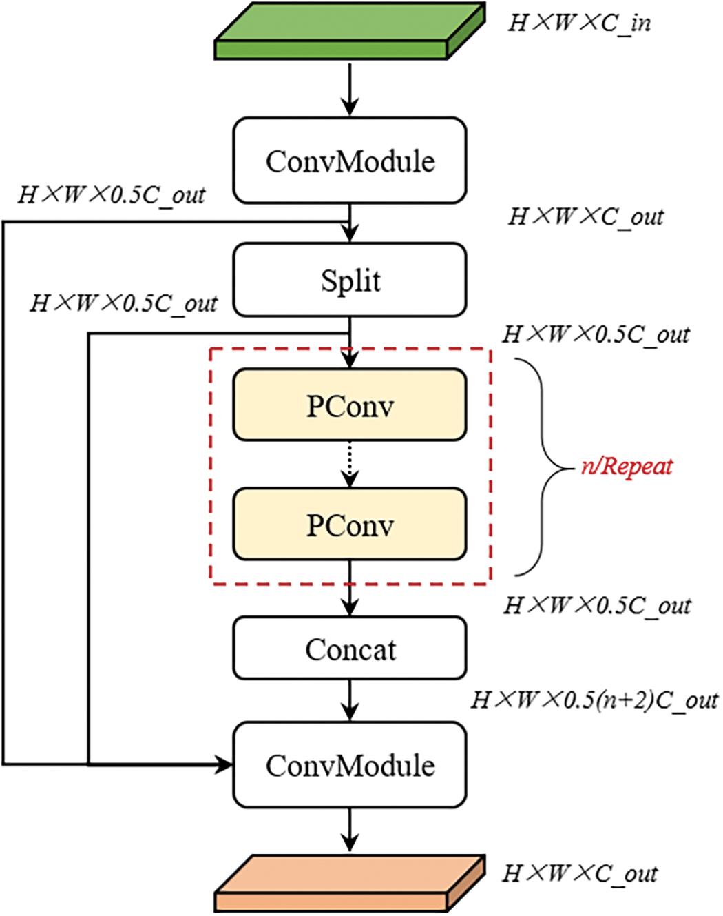
Figure 9: C2PC module structure

As can be seen from the figure above, the initial convolution block extracts the basic features of the input image. Multiple PConv modules further refine and enhance these features, while the computational load of the PConv modules themselves is low. Next, a Concat block fuses the directly passed feature maps with the processed feature maps, allowing the model to effectively utilize multi-scale and multi-level information. The final feature map is generated through the last convolution block, providing rich features for subsequent detection tasks.

3.2 Improved Network Model

To enhance the network’s detection precision, address issues of missed detections, and reduce computational resource consumption to increase detection speed, this paper implements the following steps to improve the original YOLOv8n model: First, by replacing the traditional Conv modules in the backbone with CGB modules, the model’s ability to capture critical information in images is enhanced; secondly, to further increase detection speed and precision, a Conv_GN shared convolution module design SCGD detection head is introduced, which helps address both missed detections and slow detection response; finally, to reduce the model’s parameter count and computational load, and to improve detection speed, we introduced the PConv convolution module and designed the C2PC structure. Through this series of structural optimizations and technological innovations, an improved CSC-YOLO network was constructed. This network significantly enhances processing speed and efficiency while maintaining high precision, greatly reducing the computational burden. The improved network structure, as shown in Fig. 10, effectively addresses the challenges faced by the original model in practical applications.

Figure 10: CSC-YOLO network structure

4  Experiments and Analysis

This chapter primarily outlines the experimental environment for both software and hardware, introduces the precision evaluation metrics required for preparation, and then proceeds with the experiments and analysis of the results.

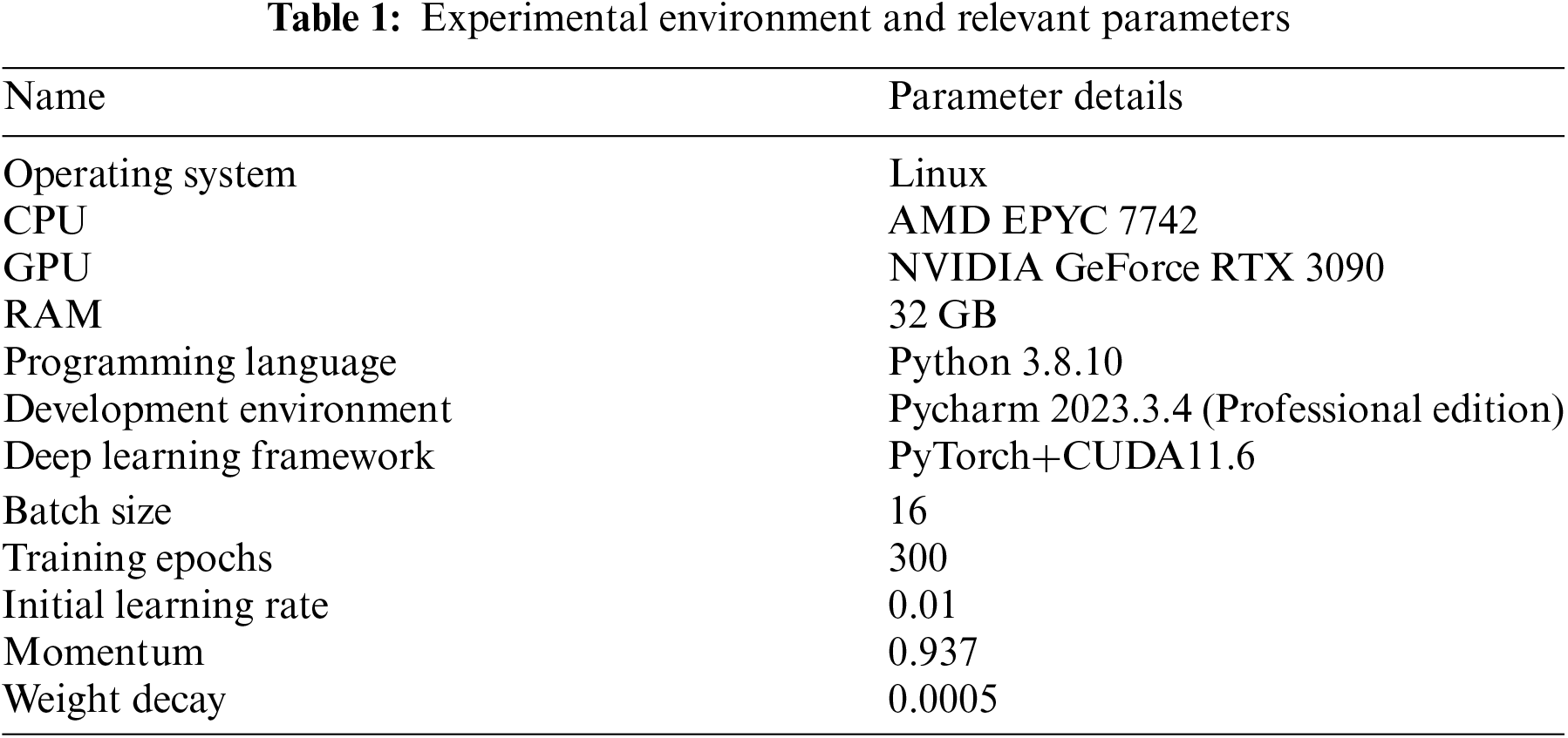
4.1 Experimental Environment and Relevant Parameters

The experimental environment in this paper is a Linux system, with an AMD EPYC 7742 CPU, an NVIDIA GeForce RTX 3090 GPU, and 32 GB of RAM. The selected compiled version of Python is Python 3.8.10. The YOLOv8 model needs to be trained under the PyTorch framework, with a batch size of 16 and a total of 300 training epochs in this experimental configuration. This is detailed in Table 1 below.

4.2 Precision Assessment Metrics

This paper verifies the performance of the improved YOLOv8n network in recognizing underwater shipwrecks using the following evaluation metrics: Precision (P), Recall (R), mean Average Precision (mAP), F1-measure (F1), floating point operations per second (FLOPs), number of Parameters (Params), frames per second (FPS), and Intersection over Union (IOU) [34,35]. The formulas are summarized from References [34,35].

In classification problems, the prediction outcomes of positive and negative samples in the network are usually divided into True Positives (TP), False Positives (FP), True Negatives (TN), and False Negatives (FN). TP denotes cases where positive samples are correctly identified as positive. FP denotes cases where negative samples are incorrectly identified as positive. TN denotes cases where negative samples are correctly identified as negative. FN denotes cases where positive samples are incorrectly identified as negative.

Precision represents the ratio of all correctly predicted positive cases to all cases identified as positive, as shown in Eq. (7).

(7)

Recall represents the ratio of all correctly predicted positive cases among the positive samples to all positive cases in the sample, as shown in Eq. (8).

(8)

In practical testing, Precision and Recall do not increase simultaneously; if one is high, the other tends to be low. For example, high precision often corresponds to low Recall. Therefore, these metrics do not clearly reflect the overall detection performance of the network. To balance Precision and Recall, the F1 can be used for a comprehensive evaluation, better balancing these precision metrics. The formula for the F1 is shown in Eq. (9).

(9)

Using Precision as the y-axis and Recall as the x-axis, a Precision-Recall (P-R) curve can be drawn. The P-R curve clearly displays the overall situation of Precision and Recall in the network’s sample set. The area under the P-R curve is known as Average Precision (AP). The calculation formula is shown in Eq. (10). A higher AP value indicates better detection performance of the network.

(10)

In situations with multiple categories, the mean of the AP values for each category is known as mAP, as shown in Eq. (11). In this study, the object is the single category of shipwrecks, so AP and mAP are equal. mAP@0.5 means the IOU threshold is 0.5; a detection box is considered correct if the overlap area with the true box exceeds 50%. mAP@0.5:0.95 represents the average of mAP at IOU intervals from 0.5 to 0.95, with steps of 0.05.

(11)

FPS is a metric used to measure the speed of image processing or model inference, commonly used to evaluate the performance of computer vision applications. FPS indicates the number of image frames processed per second. The calculation formula is shown in Eq. (12).

(12)

In the formula, “preprocess” is the preprocessing time, “inference” is the inference time, and “postprocess” is the postprocessing time.

4.3 Analysis of Experimental Results

Based on the content described in Section 4.2, this section evaluates the experiments using performance metrics such as P, R, mAP, F1, FLOPs, Params, and FPS. P represents Precision, reflecting the accuracy of the algorithm. R represents Recall, which reflects the algorithm’s rate of missed detections. F1 serves as a balanced metric between P and R. mAP, as the mean average precision, is a crucial metric that better reflects the algorithm’s performance. FLOPs and Params indicate the complexity of the algorithm. FPS reflects the detection speed of the algorithm. For each subsection, this paper selected the appropriate evaluation metrics for assessment.

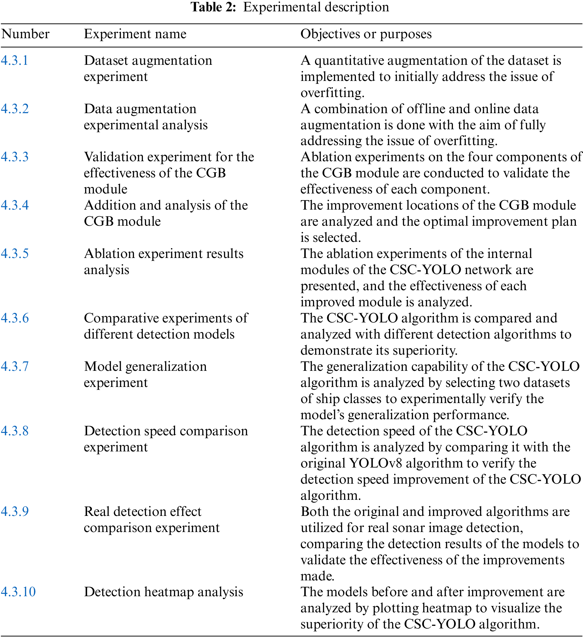
To thoroughly evaluate the performance of the CSC-YOLO algorithm, we conducted several experiments, including data augmentation, CGB module verification and addition, ablation studies of various modules, comparisons with classic advanced algorithms, model generalization tests, speed comparison on low computing power platforms, and heatmap analysis. The description of the experiments is shown in Table 2.

4.3.1 Dataset Augmentation Experiment

Overfitting refers to a model performing better on the training set than on the validation set [36]. To determine whether the dataset is large enough to avoid overfitting, this paper adopts a systematic approach: Based on the definition of overfitting, this study begins experiments with a dataset of 1000 images, then increases the dataset by 200 images at a time, repeating the experiments until the performance on the training set is equal to that on the validation set. This critical point indicates that the model has learned sufficient generalized features without overfitting the training data. The experimental results are presented in Table 3.

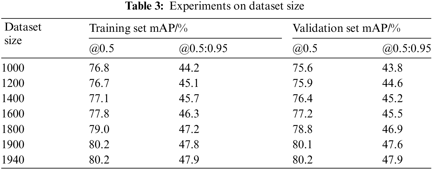
As shown in Table 3, it can be observed that data augmentation reduces the issue of overfitting. As the size of the dataset increases, the difference between the training set and the validation set gradually decreases. When the dataset was increased to 1800 images, the mAP difference between the training set and the validation set was minimal. Therefore, we increased the dataset for the experiment from 1800 to 1900 images, but we found that there was still a slight difference between the training set and the validation set. To address this issue, we reduced the number of images added, specifically adding 10 images at a time. When the total reached 1940 images, we found that the mAP values of the training set and the validation set were consistent. Therefore, we conclude that the dataset of 1940 images is the optimal dataset.

4.3.2 Data Augmentation Experimental Analysis

To address the small sample problem, this paper employs offline data augmentation techniques to expand the dataset. Specific methods include adding noise, adjusting brightness, random exposure, rotating images, flipping images, converting to grayscale, and random erasing to reconstruct the dataset. Additionally, online data augmentation using the Mosaic technique is applied to further enhance its generalization ability. These techniques are used to augment shipwreck images, increasing the number of shipwreck samples in the side-scan sonar images and improving the dataset’s generalization ability.

Through these augmentation methods, we have significantly enhanced the diversity and coverage of the dataset, thereby aiding the network in better learning and generalizing features under various conditions. To validate the effects of image enhancement, we conducted a series of experimental comparisons before and after data augmentation. Through these experiments, we have been able to clearly determine the specific impact of data augmentation techniques on model performance. The results and comparisons of the experiment are shown in Fig. 11, where Data Augmentation-1 represents offline data augmentation, and Data Augmentation-2 combines offline and online data augmentation. It demonstrates the differences in model performance before and after enhancement and verifies the effectiveness of data augmentation in improving model generalizability.

Figure 11: Before and after data augmentation comparison

The experimental results indicate that after data augmentation, there was a significant improvement in model performance. Precision increases by 13.7%, Recall by 5.1%, F1 by 8.9%, mAP@0.5 by 10.7%, and mAP@0.5:0.95 by 4.3%. The experimental results demonstrate that data augmentation enhances data diversity, allowing the network to learn a broader range of features more effectively, significantly boosting network precision and preventing overfitting due to a small dataset.

4.3.3 Validation Experiment for the Effectiveness of the CGB Module

As shown in Fig. 5, this paper conducts ablation experiments on four components of the CGB module to verify the effectiveness of the local feature extractor floc, the surrounding context extractor fsur, the joint feature extractor fjoi, and the global context extractor fglo. The effectiveness of each component is demonstrated by comparing the results after removing each part with those of the original CGB module. It is important to note that because the joint feature extractor fjoi has the function of concatenation, removing it prevents floc and fsur from being concatenated, allowing them to be used only individually. Therefore, when fjoi is removed, we also separately remove either the floc or fsur module for the experiments. Here, ‘w’ indicates that this component is used, while ‘w/o’ indicates that this component is removed. We use mAP, Params, and FLOPs as evaluation metrics, and the experimental results are presented in the Table 4.

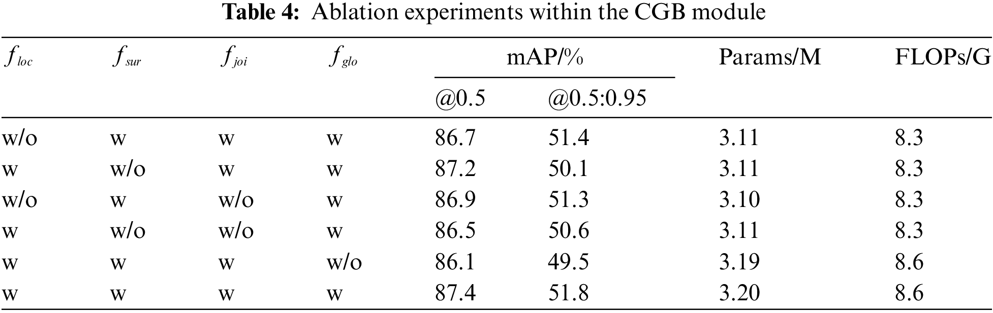
Through the ablation experiments of each component, it can be observed that removing the local feature extractor floc, the surrounding context extractor fsur, the joint feature extractor fjoi, and the global context extractor fglo leads to varying degrees of accuracy degradation, indicating that these four components are essential for the CGB module.

4.3.4 Addition and Analysis of the CGB Module

This paper explores the optimal improvement method by utilizing the CGB module in different positions. YOLOv8n-CGB employs the CGB module as a Downsampling module and enhances the Conv module to establish connections between local and global contexts, thereby accurately classifying each pixel in the image. YOLOv8n-C2f_CGB replaces the Bottleneck module in C2f with the CGB module, thereby reducing the number of parameters and computational load. Experiments were conducted on these two improvements, as shown in Table 5.

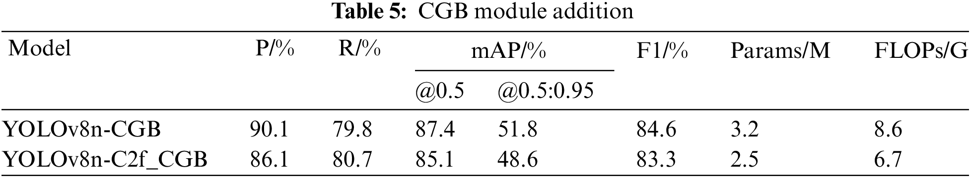
As shown in the table above, while the YOLO-C2f_CGB module can reduce the complexity of the model, its precision is less than satisfactory. The YOLOv8n-CGB outperforms YOLOv8-C2f_CGB in precision metrics. Therefore, this paper selects the YOLOv8n-CGB improvement method.

4.3.5 Ablation Experiment Results Analysis

To confirm the effectiveness of each improvement, this paper has designed a series of ablation experiments. The specific experimental setup is as follows: A represents the original YOLOv8n model; B represents the introduction of the CGB module into the model; C represents the use of the detection head SCGD; D represents the introduction of the C2PC module. The experiments are divided into eight groups, with detailed configurations and results listed in Table 6. This approach allows us to analyze in detail the specific impact of each improvement on model performance.

These eight ablation experiments demonstrate that combinations of different modules have improved performance to varying degrees, fully proving the effectiveness of this research method in enhancing the performance of side-scan sonar shipwreck image object detection. A detailed analysis of several representative experimental results follows:

Experiment 2: After introducing the CGB module, the model’s Precision increases by 1.6%, Recall by 3.3%, F1 by 2.6%, mAP@0.5 by 1.8%, and mAP@0.5:0.95 by 0.4%. The experimental results indicate that the CGB module enhances feature representation and model performance, allowing the network to learn richer feature information. However, this also leads an increasement in Parameters by 0.2 M and FLOPs by 0.4 G, which may reduce detection speed.

Experiment 5: Introducing the SCGD detection head on top of the CGB module further improves precision metrics, with Precision increasing by 0.1%, Recall by 3.5%, F1 by 2%, mAP@0.5 by 0.9%, and mAP@0.5:0.95 by 0.1%. Additionally, Parameters and FLOPs decreased by 0.6 M and 1.6 G, respectively. The experimental results indicate that Group Normalization and shared convolution operations not only enhanced the detection head’s localization and classification performance but also significantly reduced parameters and computation, increasing detection speed.

Experiment 8: Further introducing the C2PC module on top of the CGB module and SCGD detection head results in further reductions in parameters and computation. Precision increases by 0.8%, Recall slightly decreases by 0.4%, F1 increases by 0.1%, mAP@0.5 by 0.4%, and mAP@0.5:0.95 by 0.7%. Parameters decrease to 2.4 M, and FLOPs decrease to 6.3 G. The experimental results indicate that the C2PC module effectively reduces computational complexity while still efficiently extracting spatial features, enhancing the model’s overall performance.

These experimental results highlight the importance of the improvements in enhancing shipwreck detection performance and also demonstrate the potential for optimizing computational resource usage. To visually display the effects of the improvement modules in Experiments 2, 5, and 8, we performed result visualization, as shown in Fig. 12. The figure illustrates the changes in three key metrics—Loss, mAP@0.5, and mAP@0.5:0.95—during the training process.

Figure 12: Ablation experiment training comparison. (a) Loss training change curve; (b) mAP@0.5 training change curve; (c) mAP@0.5:0.95 training change curve

As seen in Fig. 12, both the original YOLOv8n model and the improved models show a gradual decrease in loss values with increasing training steps, stabilizing around 300 steps, indicating that the models have reached a good fit. Additionally, by comparing the mAP@0.5 and mAP@0.5:0.95 curves, it is evident that the improved models exhibit faster training convergence than the original model.

Comprehensive analysis of these results shows that the improved CSC-YOLO model achieved an overall increasement of 6.4% in Recall, 3.1% in mAP@0.5, and 4.7% in F1. These data strongly demonstrate that the proposed improvements significantly enhance the model’s performance in shipwreck detection, validating the effectiveness of the improvements. These enhancements not only improve the model’s performance but also optimize the training process, making the model more suitable for practical application scenarios.

4.3.6 Comparative Experiments of Different Detection Models

To further validate the superiority of the algorithm, a comparative experiment was conducted using the same dataset under identical experimental conditions. Several classical algorithms and mainstream object detection algorithms were selected for comparative experiments. The specific algorithms chosen include two-stage algorithms such as Faster-RCNN and Cascade-RCNN [37], as well as one-stage algorithms like TOOD [38], YOLOv5n [39], YOLOX-Tiny [40], YOLOv8n, YOLOv9c [41], YOLOv9t, YOLOv9s, YOLOv10 [42], RT-DETR [43], and the CSC-YOLO designed in this paper. Through systematic training and evaluation of these models, the comparative results are summarized in Table 7, providing a clear demonstration of the performance and efficiency differences of each algorithm when processing this dataset.

As shown in Table 7, it can be inferred that the algorithm proposed in this study exhibits excellent performance compared to other mainstream object detection algorithms. Notably, high-parameter models such as Faster RCNN, Cascade-RCNN, and TOOD show limited adaptability to this dataset, resulting in relatively low detection precision. Although YOLO series algorithms and the RT-DETR algorithm have advantages in terms of parameter count and computational load, their detection precision remains relatively low. In contrast, the CSC-YOLO algorithm achieves the highest detection precision while maintaining low parameter counts and computational load. Considering all factors, CSC-YOLO is a high-performance and efficient object detection algorithm that is well-suited for modern industrial applications.

4.3.7 Model Generalization Experiment

To verify the generalization capability of the CSC-YOLO algorithm, this paper selects two different types of ship datasets: one is a Synthetic Aperture Radar (SAR) dataset, and the other is an optical satellite imagery dataset. Although both are ship datasets, the image types differ significantly from the datasets used in this paper. Therefore, these two datasets are used to validate the algorithm presented in this paper.

The SAR ship dataset selected is the SAR Ship Detection Dataset (SSDD) [44]. The SSDD dataset is a single-category ship dataset with a total of 1160 images and 2456 ships, averaging 2.12 ships per image, with a high proportion of small objects, making detection challenging. The detection results are shown in Table 8: Precision increases by 0.5%, Recall by 1.8%, F1 by 0.4%, mAP@0.5 by 1.2%, and mAP@0.5:0.95 by 0.6%. The data indicate that the algorithm has a certain level of generalization capability.

The ShipRSImageNet dataset [45] was selected for optical satellite image data. The ShipRSImageNet is an optical remote sensing image dataset for ship detection and classification. It comprises 3435 images, each approximately 930 × 930 pixels, categorized into a total of 50 object classes. The recognition task was conducted using the CSC-YOLO algorithm. The detection results are presented in Table 9, with Precision increasing by 1.4%, Recall by 1.2%, F1 by 1.4%, mAP@0.5 by 1.6%, and mAP@0.5:0.95 by 0.7%. It is evident that the CSC-YOLO algorithm shows a significant improvement over the YOLOv8n algorithm in the context of optical satellite imagery.

4.3.8 Detection Speed Comparison Experiment

To verify whether the module’s lightweight processing has improved, a speed validation experiment was conducted on a resource-limited device platform, using an NVIDIA GeForce RTX 3050Ti mobile device. The results are listed in Table 10.

By applying Eq. (12), we obtained the FPS value. As shown in the results table, compared to the original YOLOv8n model, the CSC-YOLO model reduces the number of parameters by 20% and the computational load by 23.2%, while increasing the FPS value by 17.6%. These indicate that the detection network constructed in this paper can achieve real-time detection on a low computing power mobile GPU, effectively enhancing detection efficiency and speed.

The GPU used in this experiment is the GeForce RTX 3050 Ti mobile graphics card, which has a power consumption of 80W and a computing speed of 7.2 TFLOPs. Devices such as unmanned ships and AUVs typically can only accommodate low-power devices. For example, the NVIDIA Jetson TX2 embedded edge computing device can achieve a computing speed of 1.33 TFLOPs at a power consumption of 7.5W [46], which is about one-fifth of the computing speed of the 3050 Ti. If the detection model constructed in this paper is deployed on such a device, even with one-fifth of the detection speed, it can still meet the requirements for real-time detection.

4.3.9 Real Detection Effect Comparison Experiment

Three challenging side-scan sonar shipwreck images were selected for the detection task. Fig. 13 shows the comparison of shipwreck object detection results before and after the improvements, from top to bottom: the original image, the annotated image, the detection result of the YOLOv8n model, and the detection result of the CSC-YOLO model. This intuitive comparison clearly demonstrates the performance differences between the two models in shipwreck object detection. Such visual representation helps evaluate and understand the specific effects of the improvements, highlighting the advantages of the CSC-YOLO model, especially in scenarios that are challenging for the original model.

Figure 13: Comparison of model detection results before and after improvement. (a) Original image; (b) Annotated imaged; (c) YOLOv8n detection image; (d) CSC-YOLO detection image

From the analysis of Fig. 13, the original YOLOv8n model tends to miss small objects, especially in complex underwater environments where it struggles to accurately identify shipwreck objects, leading to frequent false detections. Although it can detect overlapping objects, its localization precision and confidence are not at an ideal level. Compared to the original model, the proposed CSC-YOLO model shows significant improvements in both localization precision and confidence. In the first and third sets of experiments, it effectively mitigated the issue of missed detections. In the second set of experiments, it significantly reduced false detections, making the model’s shipwreck detection more accurate and detailed, with detection boxes better fitting the object contours.

4.3.10 Detection Heatmap Analysis

During the training process of network models, the semantic information of lower-level feature maps is often not easily visualized. To gain deeper insights into the model’s focus on features during detection, this paper employs Gradient-weighted Class Activation Mapping (Grad-CAM) technology [47]. This technique generates heatmaps by calculating gradients on feature maps, thereby visualizing the model’s attention points during the recognition process.

The heatmaps generated before and after the model improvements are shown in Fig. 14. In these heatmaps, red areas indicate the highest attention of the model, yellow areas indicate high attention, and blue areas represent regions with minimal impact on the model’s recognition process, often considered redundant information. By comparing the heatmaps before and after the improvements, one can visually observe the changes in the model’s focus on features and assess the effectiveness of the optimizations.

Figure 14: Heatmap comparison before and after improvement. (a) Original image; (b) YOLOv8n; (c) CSC-YOLO

From the Grad-CAM generated heatmaps, it can be seen that the original YOLOv8 model has a relatively scattered focus on shipwreck objects, with almost no significant attention on small objects. In complex environments, the focus areas are overly dispersed, leading to erroneous detections. This indicates that the original model may have difficulties handling complex or small objects.

In contrast, the CSC-YOLO model’s main focus areas are concentrated on the object locations, showing better focusing capability. This concentration of attention helps avoid interference from environmental factors, effectively preventing false detections and missed detections. By optimizing the attention points, CSC-YOLO improves detection precision and reliability, especially in cases where the objects are small or the background is complex. These improvements make CSC-YOLO an ideal choice for handling challenging detection tasks.

5  Conclusion

In the task of detecting shipwrecks in side-scan sonar images, the complex underwater environment poses significant limitations, leading to low detection precision and slow detection speeds. In this study, to address the small sample problem, this paper performs offline data augmentation based on the imaging characteristics of side-scan sonar shipwreck images, thereby expanding the dataset and increasing sample diversity. And this method enhances the model’s generalization capability through the integrated Mosaic algorithm. Furthermore, we address the issues of low detection precision and low detection speeds in side-scan sonar shipwreck image detection by proposing an improved YOLOv8 network-based method. By introducing the CGB module into the backbone network, the method enhances the network’s ability to learn and express image features, improving feature extraction and making shipwreck images easier to detect. Additionally, by using Group Normalization technology and shared convolution operations, we designed the SCGD detection head, which significantly reduces parameters and computational load while improving localization and classification performance. Using the C2f structure and PConv convolution, we constructed the C2PC module, which helps the network maintain effective spatial feature extraction while reducing computational complexity. The improvements mentioned above have led to the following enhancements in the CSC-YOLO model: Precision increases by 2.5%, Recall increases by 6.4%, mAP@50 increases by 3.1%, mAP@50:95 increases by 1.2%, and F1 rises by 4.7. Additionally, the computational load decreases by 20%, the parameter count reduces by 23.2%, and FPS increases by 17.6%. This model achieves a good balance between detection precision, detection speed, and model structure, meeting the demand for model light-weighting in engineering deployments. This model can be applied to searching shipwrecks in complex sea areas.

Acknowledgement: The authors thank the financial support of the Hainan Provincial Natural Science Foundation (Grant No. 420CXTD439), Sanya Science and Technology Special Fund (Grant No. 2022KJCX83), Institute and Local Cooperation Foundation of Sanya in China (Grant No. 2019YD08), and National Natural Science Foundation of China (Grant No. 61661038). We would also like to thank all the reviewers for their suggestions.

Funding Statement: This work is supported in part by the Hainan Provincial Natural Science Foundation (Grant No. 420CXTD439), Sanya Science and Technology Special Fund (Grant No. 2022KJCX83), Institute and Local Cooperation Foundation of Sanya in China (Grant No. 2019YD08), and National Natural Science Foundation of China (Grant No. 61661038).

Author Contributions: Study conception and design: Shengxi Jiao, Fenghao Xu, Haitao Guo; Data support: Haitao Guo; Analysis and interpretation of results: Shengxi Jiao, Fenghao Xu, Haitao Guo; Drafting of the manuscript: Fenghao Xu. All authors reviewed the results and approved the final version of the manuscript.

Availability of Data and Materials: The public SSDD dataset can be found at the following URL: https://github.com/TianwenZhang0825/Official-SSDD (accessed on 20 November 2024). The public ShipRSImageNet dataset can be found at the following URL: https://github.com/MatthewInkawhich/ShipRSImageNet (accessed on 20 November 2024). Data and materials supporting the findings of this study can be requested from the authors upon acceptance.

Ethics Approval: The authors declare that there are no ethical or moral issues in violation related to this study.

Conflicts of Interest: The authors declare no conflicts of interest to report regarding the present study.

References

1. J. Zhao, Z. Lu, and A. Wang, “Development status of marine surveying and mapping technology,” (in ChineseJ. Geomat., vol. 42, no. 6, pp. 1–10, Sep. 2017. doi: 10.14188/j.2095-6045.2017312. [Google Scholar] [CrossRef]

2. L. Janowski, M. Kubacka, and A. Pydyn, “From acoustics to underwater archaeology: Deep investigation of a shallow lake using high-resolution hydroacoustics-The case of Lake Lednica,” Archaeometry, vol. 63, no. 5, pp. 1059–1080, Oct. 2021. doi: 10.1111/arcm.12663. [Google Scholar] [CrossRef]

3. L. Character, A. Ortiz, T. Beach, and S. Luzzadder-Beach, “Archaeologic machine learning for shipwreck detection using lidar and sonar,” Remote Sens., vol. 13, no. 9, May 2021, Art. no. 1759. doi: 10.3390/rs13091759. [Google Scholar] [CrossRef]

4. Q. Zhuang, G. Gong, and D. Zhou, “Novel wreck salvaging method using curved rectangular pipe basing method: A case study of “Yangtze River Estuary II” ancient shipwreck salvage project,” Undergr. Space, vol. 18, no. 11, pp. 97–113, Oct. 2024. doi: 10.1016/j.undsp.2023.11.016. [Google Scholar] [CrossRef]

5. Z. Gu, “Rescue of inland waterway shipwrecks,” (in ChineseCity Disas. Reduct., vol. 2023, no. 6, pp. 34–39, Nov. 2023. [Google Scholar]

6. S. Li, Y. Zhang, and J. Zhao, “A comprehensive buried shipwreck detection method based on 3-D SBP data,” IEEE J. Oceanic Eng., vol. 49, no. 2, pp. 458–473, Apr. 2024. doi: 10.1109/JOE.2023.3318793. [Google Scholar] [CrossRef]

7. M. Lee, J. Y. Jung, K. C. Park, and S. H. Choi, “Environmental and economic loss analyses of the oil discharge from shipwreck for salvage planning,” Mar. Pollut. Bull., vol. 155, Jun. 2020. doi: 10.1016/j.marpolbul.2020.111142. [Google Scholar] [PubMed] [CrossRef]

8. H. -T. Nguyen, E. -H. Lee, and S. Lee, “Study on the classification performance of underwater sonar image classification based on convolutional neural networks for detecting a submerged human body,” Sensors, vol. 20, no. 1, Jan. 2020, Art. no. 94. doi: 10.3390/s20010094. [Google Scholar] [PubMed] [CrossRef]

9. Y. Tang, L. Wang, and S. Jin, “AUV-based side-scan sonar real-time method for underwater-object detection,” J. Mar. Sci. Eng., vol. 11, no. 4, Mar. 2023, Art. no. 690. doi: 10.3390/jmse11040690. [Google Scholar] [CrossRef]

10. B. Shi, T. Cao, and Q. Ge, “Sonar image intelligent processing in seabed pipeline detection: Review and application,” Meas. Sci. Technol., vol. 35, no. 4, Jan. 2024. doi: 10.1088/1361-6501/ad1919. [Google Scholar] [CrossRef]

11. Z. Dong, Y. Liu, L. Yang, and Y. Feng, “Artificial reef detection method for multibeam sonar imagery based on convolutional neural networks,” Remote Sens., vol. 14, no. 18, Sep. 2022, Art. no. 4610. doi: 10.3390/rs14184610. [Google Scholar] [CrossRef]

12. T. Wang, G. Pan, and J. Zhang, “A study on seafloor substrate classification based on texture features of side-scan sonar images,” in Proc. 2020 Western China Acoustic Acad. Exchange Conf., China, Aug. 20, 2020, pp. 403–406. [Google Scholar]

13. A. Aub and R. Diamant, “CFAR detection algorithm for objects in sonar images,” IET Radar Sonar Navig., vol. 14, no. 1, pp. 1757–1766, Nov. 2020. doi: 10.1049/iet-rsn.2020.0230. [Google Scholar] [CrossRef]

14. R. Girshick, J. Donahue, T. Darrell, and J. Malik, “Rich feature hierarchies for accurate object detection and semantic segmentation,” 2014, arXiv:1311.2524. [Google Scholar]

15. S. Ren, K. He, R. Girshick, and J. Sun, “Faster R-CNN: Towards real-time object detection with region proposal networks,” 2016, arXiv:1506.01497. [Google Scholar]

16. N. Carion, F. Massa, and G. Synnaeve, “End-to-end object detection with transformers,” 2020, arXiv:2005.12872. [Google Scholar]

17. J. Redmon, S. Divvala, and R. Girshick, “You only look once: Unified, real-time object detection,” 2016, arXiv:1506.02640. [Google Scholar]

18. D. Williams, “Underwater object classification in synthetic aperture sonar imagery using deep convolutional neural networks,” in Proc. 2016 23rd Int. Conf. Pattern Recognit. (ICPR), Dec. 4–8, 2016. [Google Scholar]

19. J. Choi Kim and H. Kwon, “The application of convolutional neural networks for automatic detection of underwater object in side scan sonar images,” J. Acoust. Soc. Korea, vol. 37, no. 2, pp. 118–128, Apr. 2018. doi: 10.7776/ASK.2018.37.2.118. [Google Scholar] [CrossRef]

20. J. Kim and S. Yu, “Convolutional neural network-based real-time ROV detection using forward-looking sonar image,” in Proc. 2016 IEEE/OES Autonom Underwater Veh. (AUV), Nov. 6–9, 2016, pp. 396–400. [Google Scholar]

21. Y. Wu, “Sonar image object detection and recognition based on convolution neural network,” Mobile Inf. Syst., vol. 2021, no. 1, Mar. 2021. doi: 10.1155/2021/5589154. [Google Scholar] [CrossRef]

22. Y. Tang, H. Li, and W. Zhang, “Lightweight DETR-YOLO method for detecting shipwreck object in side-scan sonar,” (in ChineseSyst. Eng. Electron., vol. 44, no. 8, Mar. 2021. [Google Scholar]

23. F. Zhang, W. Zhang, and C. Cheng, “Detection of small objects in side-scan sonar images using an enhanced YOLOv7-based approach,” J. Mar. Sci. Eng., vol. 11, no. 11, Nov. 2023, Art. no. 2155. doi: 10.3390/jmse11112155. [Google Scholar] [CrossRef]

24. S. Fu, F. Xu, and J. Liu, “Underwater small object detection in side-scan sonar images based on improved YOLOv5,” in Proc. 2022 3rd Int. Conf. Geology, Mapping Remote Sensing (ICGMRS), Apr. 22–24, 2022, pp. 446–453. [Google Scholar]

25. S. Woo, J. Park, J. Lee, and I. Kweon, “CBAM: Convolutional block attention module,” 2018, arXiv:1807.06521. [Google Scholar]

26. J. Nelson and B. Dwyer, “Roboflow: Give your software the power to see objects in images and video,” 2020. Accessed: Dec. 14, 2023. [Online]. Available: https://roboflow.com [Google Scholar]

27. T. DeVries and G. W. Taylor, “Improved regularization of convolutional neural networks with cut-out,” 2017, arXiv:1708.04552. [Google Scholar]

28. C. Chen, M. Y. Liu, and O. Tuzel, “R-CNN for small object detection,” in Proc. Comput. Vis.-ACCV 2016: 13th Asian Conf. Comput. Vis., Nov. 20–24, 2016, pp. 214–230. [Google Scholar]

29. A. Bochkovskiy, C. Y. Wang, and H. Y. M. Liao, “YOLOv4: Optimal speed and accuracy of object detection,” 2020, arXiv:2004.10934. [Google Scholar]

30. G. Jocher, “Ultralytics YOLO,” 2023. Accessed: Aug. 21, 2023. [Online]. Available: https://github.com/ultralytics/ultralytics [Google Scholar]

31. T. Wu, S. Tang, and R. Zhang, “CGNet: A light-weight context guided network for semantic segmentation,” 2019, arXiv:1811.08201. [Google Scholar]

32. Y. Wu and K. He, “Group normalization,” 2018, arXiv:1803.08494. [Google Scholar]

33. J. Chen, S. Kao, and H. He, “Run, don’t walk: Chasing higher FLOPS for faster neural networks,” 2023, arXiv:2303.03667. [Google Scholar]

34. R. Kaur and S. Singh, “A comprehensive review of object detection with deep learning,” Digit. Signal Process., vol. 132, Jan. 2023, Art. no. 103812. doi: 10.1016/j.dsp.2022.103812. [Google Scholar] [CrossRef]

35. J. Redmon and A. Farhadi, “YOLO9000: Better, faster, stronger,” 2016, arXiv:1612.08242. [Google Scholar]

36. O. A. Montesinos López, A. Montesinos López, and J. Crossa, “Overfitting, model tuning, and evaluation of prediction performance,” Multivar. Statist. Mach. Learn. Methods Genomic Predict., pp. 109–139, Jan. 2022. doi: 10.1007/978-3-030-89010-0_4. [Google Scholar] [CrossRef]

37. Z. Cai and N. Vasconcelos, “Cascade R-CNN: Delving into high quality object detection,” 2017, arXiv:1712.00726. [Google Scholar]

38. C. Feng, Y. Zhong, and Y. Gao, “TOOD: Task-aligned one-stage object detection,” 2021, arXiv:2108.07755. [Google Scholar]

39. G. Jocher, “YOLOv5 by Ultralytics. 2020,” Accessed: Apr. 11, 2024. [Online]. Available: https://github.com/ultralytics/yolov5 [Google Scholar]

40. Z. Ge, S. Liu, F. Wang, Z. Li, and J. Sun, “YOLOX: Exceeding YOLO series in 2021,” 2021, arXiv:2107.0843. [Google Scholar]

41. C. -Y. Wang, I. -H. Yeh, and H. -Y. Liao, “YOLOv9: Learning what you want to learn using programmable gradient information,” 2024, arXiv:2402.13616. [Google Scholar]

42. A. Wang, H. Chen, and L. Liu, “YOLOv10: Real-time end-to-end object detection,” 2024, arXiv:2405.14458. [Google Scholar]

43. Y. Zhao, W. Lv, and S. Xu, “DETRs beat YOLOs on real-time object detection,” 2024, arXiv:2304.08069. [Google Scholar]

44. S. Li, X. Li, and Z. Song, “Multi scale SAR image detection algorithm for ships based on improved YOLOv5,” (in ChineseJ. Data Acquisit. Process., vol. 39, no. 1, pp. 120–131, Jan. 2024. doi: 10.16337/j.1004-9037.2024.01.011. [Google Scholar] [CrossRef]

45. Z. Zhang, L. Zhang, and Y. Wang, “ShipRSImageNet: A large-scale fine-grained dataset for ship detection in high-resolution optical remote sensing images,” IEEE J. Sel. Top. Appl. Earth Obs. Remote Sens., vol. 14, pp. 8458–8472, Aug. 2021. doi: 10.1109/JSTARS.2021.3104230. [Google Scholar] [CrossRef]

46. Y. Zheng, “Side scan sonar image object detection method based on improved YOLOv5 network,” (in ChineseHydrograp. Survey. Chart., vol. 42, no. 4, pp. 18–21, Jul. 2022. doi: 10.3969/j.issn.1671-3044.2022.04.005. [Google Scholar] [CrossRef]

47. M. Danelljan, F. S. Khan, and M. Felsberg, “Adaptive color attributes for real-time visual tracking,” in Proc. IEEE Conf. Comput. Vis. Pattern Recognit. (CVPR), Jun. 23, 2014, pp. 1090–1097. [Google Scholar]