Federated Learning’s Role in Next-Gen TV Ad Optimization

1  Introduction

1.1 General Context of Ad Scheduling Using Federated Learning

Optimizing TV ad schedules involves complex decision-making processes, where broadcasters must consider various factors, including ad placement, viewer engagement metrics and category performance [1,2]. Traditionally, this optimization is done locally, within the constraints of each broadcaster’s available data, leading to missed opportunities for deeper insights that could be gained from a wider dataset. In the context of optimizing TV ad schedules, the utilization of sensitive data plays a significant role in making informed decisions that maximize viewer engagement and advertising revenue [3]. Each TV station, as a client in the Federated Learning (FL) framework, leverages its dataset comprising various characteristics of data used to allocate spots in advertising breaks. FL is a decentralized approach to ML where algorithms are trained across numerous devices or servers, each holding its own data, without actually sharing this data [4]. This method is key for protecting privacy and minimizing the necessity for data centralization and transmission, proving particularly useful in sectors such as healthcare, finance and on personal devices [5]. It kicks off with a global model being initialized on a central server, which is then sent out to various devices for local training on their specific data. Only the updates from this training, like weights and gradients, are sent back to the central server, ensuring the actual sensitive data remains on the device. The central server then aggregates these updates to refine the global model. This process of local training, update transmission and aggregation, is repeated multiple times to boost the model’s accuracy [6].

One of the standout features of FL is its commitment to data privacy, as it ensures that sensitive information does not leave its original location. Additionally, it is bandwidth-efficient, transmitting only model updates instead of the data itself. This method not only enhances model performance by learning from various data sources and distributions, but also aligns with edge computing by facilitating local data processing [7]. Nonetheless, FL comes with its set of challenges, including the significant communication overhead from sending model updates, variability in data across devices (statistical heterogeneity), differences in devices’ computational capabilities (system heterogeneity) and emerging security threats like model poisoning and inference attacks. These issues call for strong defense strategies to maintain the security and effectiveness of FL frameworks [8].

1.2 Practical Implementation and Advantages of FL

In practical terms, FL has been implemented in mobile devices for improving predictions, in the healthcare industry to collaboratively develop disease prediction and treatment models without exchanging patient information [9,10] and in the finance sector for enhancing fraud detection and risk management. By enabling the creation of powerful models while safeguarding user privacy, FL is emerging as an essential technology in today’s data-sensitive environment.

Broadcasters significantly benefit from FL when scheduling TV ads by leveraging a ML approach that trains models across multiple decentralized devices or servers without exchanging local data samples. This method enhances targeting and personalization by analyzing viewership patterns and preferences across different households while keeping the data localized, allowing ads to be more closely aligned with specific audience segments’ interests and behaviors without compromising viewer privacy. Furthermore, FL enables broadcasters to gain real-time or near-real-time insights into viewership trends and ad performance, making it possible to dynamically adjust ad scheduling based on current data. This optimization ensures ads are placed in time slots where they are likely to have the most impact. The integration of data from various sources, including set-top boxes, smart TVs and mobile devices, without directly sharing the data, aids in creating a comprehensive understanding of a viewer’s preferences across different viewing platforms [11]. This strategic ad scheduling accounts for multi-platform viewing habits.

As mentioned, one of the key benefits of FL is its ability to enhance privacy and data security [12]. By keeping the data localized and not requiring centralization, it addresses privacy concerns and complies with data protection regulations like GDPR and CCPA. Additionally, the reduction in the need for extensive data transmission leads to more efficient use of bandwidth and lower data handling costs, which is advantageous for broadcasters dealing with large volumes of viewership data. FL also facilitates collaborative model training across different broadcasters and networks without sharing raw data. This industry-wide collaboration leads to insights on viewership patterns and ad effectiveness, helping broadcasters to schedule ads more effectively while maintaining competitive confidentiality. By leveraging FL, broadcasters increase the relevance and effectiveness of their ad placements, benefiting both advertisers and viewers through improved targeting, enhanced privacy and operational efficiency.

1.3 The Challenge of Scheduling Ads

TV stations face the challenge of scheduling a multitude of ads within a finite number of slots, each with its unique viewer demographics, engagement rates and associated costs. The objective is to arrange these ads in a way that maximizes total revenue (the spots that pay the most should be placed first or last in the break) and maximizes viewer engagement. This step establishes a baseline for effective scheduling of the spots. For the local optimization problem, the data used for each break usually consists of the index, cost, length of the spot and the category.

When advertisements are positioned manually in commercial breaks, the process incorporates a personal touch, relying on the intuition and industry knowledge of the schedulers. This method allows for immediate decisions and adjustments based on a nuanced understanding of the audience and programming content. However, this approach can be time-consuming and less responsive to rapid changes in viewer behavior or program popularity, potentially leading to less efficient use of advertising slots. Consequently, the traditional strategy of manual ad placement faces significant challenges in maximizing the effectiveness and efficiency of advertising campaigns, underscoring the advantages of automated systems. Optimizing commercial breaks has become a sophisticated endeavor, integrating a blend of strategies, technologies and creative approaches to maximize viewer engagement and advertising revenue. The evolution of these tactics reflects an industry striving to balance the demands of advertisers, the expectations of viewers and the operational realities of broadcasting. Research indicates that ads are more frequent towards the end of programs, with longer breaks aligned with more popular television content to capture maximum audience attention. This tactic leverages viewer engagement patterns, ensuring that advertisements reach a broad audience at moments of peak interest [13].

1.4 Objective, Novelty and Structure of the Paper

In this paper, the objective is to optimize television advertising schedules to maximize viewer engagement and revenue while addressing the challenges posed by traditional methods that operate in isolation and concerns over privacy and data sharing. This is achieved through a novel approach that leverages FL to enhance TV ad schedule optimization. This approach combines local optimization techniques with global ML models to uncover actionable insights without compromising data privacy, utilizing a mix of linear programming and ML, specifically a KNN model, for ad spot positioning and predicting new entries’ positions.

The novelty of this approach consists in implementing scheduling at a large scale and enhances predictive accuracy and strategic insight across different networks while preserving data privacy. The scheduling process starts with linear programming for the initial optimization of ad schedules, followed by the use of a KNN model to predict the placement of ads within the schedule. Given the complexity of the ad-scheduling landscape, the proposed solution uses a two-phase prescriptive-predictive framework. Initially, ad placements are optimized using Google’s OR-Tools CP-SAT, ensuring that the final schedule is based on the results of the optimization. In the subsequent step, the generated schedule serves as a reference for a predictive task, which determines the placement of additional ads based on their attributes, facilitating scalability (with models like KNN, Light Gradient Boosting Machine and Random Forest). In addition, the use of FL improves predictive performance and provides comprehensive insights across different broadcasting networks, while protecting data confidentiality.

The current research is structured into several sections. The introduction outlines the general context of ad scheduling with FL, highlighting its practical applications, benefits and challenges, as well as the objective and novelty of the proposed approach. Section 2 provides a literature review, offering a comparative analysis of existing methods in tabular format. Section 3 details the research method, including the flowchart, input data, optimization process, prediction models including KNN, the post-processing step in KNN and the steps involved in FL. In Section 4, the results are presented in alignment with the methodology. The final sections cover discussions and conclusions.

2  Literature Review

Since 1998, Reference [14] introduced SPOT (Scheduling Programs Optimally for Television), a cutting-edge analytical framework designed for crafting optimal schedules for prime-time television programming. The emergence of numerous cable TV channels has sharply escalated the battle for viewer ratings. The efficacy of SPOT was demonstrated using data from the first quarter of 1990 from a cable network, where its application suggested a potential to boost overall profitability by roughly 2%, equating to an annual increase of over $6 million for the network. Furthermore, the complexity of optimizing allocations within a multi-constraint environment has been presented in [15]. It presents a problem faced by Channel 4, a British TV corporation which earns a significant portion of its revenue from campaign advertisements shown during commercial breaks. To tackle the scheduling problem, Mixed Integer Programming (MIP) was used. The solution proposed for Channel 4 uses both optimization and heuristic methods to find the optimal spot positions. However, this method is very complex and could involve millions of decisions and restrictions to consider. In their research, Reference [16] delved into the critical operational task of scheduling advertisements or spots, a daily necessity in the television industry that plays a pivotal role in distributing viewers across advertisers. The research introduced a pragmatic approach that combined mathematical programming with time series analysis to craft daily schedules primed for broadcast. Another research introduced an innovative scheduling algorithm designed to efficiently and cost-effectively allocate a Bag of Tasks (BoT) across Virtual Machines (VMs) within cloud computing environments [17]. Through comparative analysis against contemporary benchmark algorithms such as Round Robin, First Come First Serve, Ant Colony Optimization and Genetic Algorithm, the study’s findings highlighted the superior performance of the proposed scheduling algorithm.

Additionally, Reference [18] explored the rapidly growing trend of advertising spending on online video streaming services, which have become a staple in a majority of US households. Unlike traditional linear TV, these streaming platforms offer viewers the flexibility to consume content in a non-linear fashion, such as binge-watching. To address this gap, the authors proposed a novel three-stage approach aimed at crafting an optimal advertising schedule that harmonized the viewer’s content consumption experience with the streaming service’s advertising objectives. Also, Reference [19] explored the challenge of automating the intricate process of advertisement scheduling in broadcast television networks. Unlike traditional methods, their approach accounted for the dynamic nature of ad slot requests, which were not always submitted simultaneously, and seek to streamline the extensive negotiations often required to align the interests of TV networks and advertisers. To address these challenges, the authors introduced a novel data-driven strategy that combined intention learning with mathematical optimization and clustering techniques to mimic the expert schedulers’ decision-making processes. This approach automated ad scheduling through mathematical programming, while expert goals and limitations were identified from past examples using inverse optimization.

Researchers [20] delved into the complex issue of allocating commercial advertisements within TV breaks, a task recognized as NP-hard and characterized as a multi-stakeholder, multi-objective problem with conflicting goals among different brands and a variety of constraints. The challenge consisted in finding solutions that align with a decision maker’s specific area of interest within the Pareto Optimal Front, a frontier representing the most efficient trade-offs between competing objectives. Introducing a new solution, the RAGE-MOEA approach, the authors proposed a method that synergized the diversity strengths of AGE-MOEA with the focused convergence of reference-based strategies. In their study, Reference [21] addressed the complex multi-objective optimization problem facing advertising agencies in the context of TV advertising. This challenge revolved around selecting appropriate commercial breaks for airing ads from various brands, aiming to maximize the reach or Gross Rating Point (GRP) for these brands while adhering to budget limitations, brand competition and scheduling constraints. To tackle this issue, the authors proposed a multi-objective integer programming model and introduced algorithms designed to generate solutions that were Pareto-optimal, meaning they represented the most efficient trade-offs among the competing objectives. Furthermore, Reference [22] tackled the challenges inherent in the markets for television advertising time slots by proposing a novel combinatorial auction format. This format was designed to address the difficulties of approximating core-selecting payments for complex problems, a critical issue given the vast size and complexity of actual ad markets. The authors introduced a more compact bidding language specifically tailored for advertising, focusing on coverage or demographic reach. Additionally, Reference [23] delved into specific techniques aimed to deliver highly specific messages to narrowly defined audience segments. Despite the purported effectiveness of microtargeting strategies, there were debates about their cost-effectiveness, especially concerning optimizing impressions within a fixed budget. In another study, Reference [24] explored the complex campaign allocation problem associated with placing commercial advertisements within TV breaks, framing it as a multi-stakeholder, multi-objective issue characterized by competing objectives among different brands and a multitude of constraints. Recognized as an NP-hard problem, it presented challenges not only due to its high dimensional objective space, but also in terms of scalability related to the number of advertising breaks. The authors introduced an innovative approach employing R-NSGA-II, a Many-Objective Evolutionary Algorithm (MaOEA), enhanced with a unique gene encoding/decoding process.

Moreover, Reference [25] delved into the interplay between TV advertising and its impact on consumers’ online behavior, highlighting the challenges firms face in aligning TV ads with real-time online marketing efforts. Collaborating with an online travel platform, they conducted a field experiment comparing regions exposed to TV ads with control regions. Their findings, through a synthetic difference-in-differences analysis, revealed an immediate uptick in online browsing and sales following TV advertising. Reference [26] addressed the evolving landscape of targeted advertising across various platforms, emphasizing the importance of sophisticated planning models for ad networks tasked with aligning ads with specific audience segments. He introduced the concept of Guaranteed Targeted Display Advertising (GTDA), covering a range of media from webpage banners to digital TV, and proposed a transportation problem model with a quadratic objective to navigate the GTDA planning challenge. By incorporating audience uncertainty and forecast errors, Turner identified conditions under which the quadratic objective effectively represents ad delivery performance metrics. He presented two algorithms for tackling large-scale problems: one that progressively refined audience segments and another that scaled to find feasible solutions within set audience partitions. Exploring the immediate impact of TV advertisements on online brand and price searches, Reference [27] focused on enhancing the assessment of TV commercials based on their instant influence on crucial online behaviors. The study combined data on brand and price searches, measured minute-by-minute, with detailed information on TV ad placements for the top three pickup truck brands in the US over a period of 11 months. A versatile modeling approach was introduced, facilitating the measurement of the direct online reactions following TV ad broadcasts.

Programmatic television advertising technologies give advertisers the ability to track competitor ad placements and adjust their own ads almost instantly [2]. The researchers explored how managers can enhance the efficiency of their ad schedules by strategically positioning their ads in relation to competitor ads. By analyzing a dataset of over 43,000 ads for the focal brand and 49,000 competitor ads, they evaluated the impact of four ad scheduling approaches on online conversion rates. The most effective tactic was to schedule ads during periods when competitors are not advertising or on different channels, which optimizes ad performance and captures conversions that might otherwise go to competitors. If avoiding competitor ads is not feasible, brands should aim to advertise more frequently than their competitors. This approach reduced the negative impact of competitor ads, where competitor exposure dilutes the effectiveness of own-brand advertising. Their results showed that the use of programmatic TV advertising could have enabled the firm to increase conversions from television ads by 59%.

Another research addressed the inefficiencies of manual radio ad scheduling by proposing an automated approach using genetic algorithms [28]. The study focused on optimizing ad playback schedules for a 12-h broadcast day, divided into prime time (4–8 AM, 6–10 PM) and regular time. Ads were scheduled every 15 min, with a maximum of 76 ads per day. The rules limited each ad to a maximum of 5 plays during prime time and 8 during regular time, ensuring effective reach without overexposure. Genetic algorithms were used to automate the scheduling process by creating and refining schedules through chromosome initialization, selection, crossover and mutation. The fitness of each schedule was based on minimizing rule violations, such as exceeding the maximum number of daily plays or double-booking ads in the same time slot. The algorithm achieved an 83.79% accuracy in creating optimized ad schedules, leading to more effective ad placements throughout the day.

Furthermore, Reference [29] presented comprehensive research of the algorithmic challenges involved in scheduling space-sharing for Internet advertising. The scheduling problem required that each ad, defined by its geometry and display frequency, was scheduled so that it met three criteria: correct display frequency, sufficient space for its geometry and simultaneous arrangement of ads within the available space. The authors introduced a new variant of the bin packing problem to solve it, where multiple copies of each item (ad) must be placed in separate bins. Furthermore, an efficient algorithm was proposed to find the optimal solution for a restricted version of this problem, while a 2-approximation algorithm was provided for the unrestricted case. This approximation was applied to optimize space usage and determine the best subset of ads to display under space constraints. Additionally, the paper addressed an online version of the ad scheduling problem, where ad space requests arrived sequentially, and decisions must be made in real-time.

Additionally, the advertisement placement problem involved efficiently managing both space and time for ads displayed on the Internet, such as on a web page’s banner [30]. Multiple small ads could be displayed side by side simultaneously, or a schedule could rotate through different ads at different times. Advertisers specified the size of their ad and how often it should appear in each cycle. The scheduler could choose to accept or reject any ad but must ensure that all accepted ads fit within the available space and time constraints. Each ad was associated with a non-negative profit, and the goal is to maximize the total profit by scheduling the best subset of ads. Furthermore, Reference [31] approached the optimal scheduling and placement of Internet ads.

Online banner advertising, a common form of web advertising, relies on effective scheduling to maximize outcomes like click-through rates [32]. The researchers presented a model for scheduling online banner ads, introducing an objective function that incorporated four key factors affecting ad performance. It offered both an integer programming model with a non-linear objective and two solution approaches: heuristic and meta-heuristic algorithms. The heuristic method effectively established strong lower and upper bounds by leveraging model properties. Tests on random and standard datasets demonstrated the efficiency of these algorithms, particularly in finding tighter bounds for specific ad specifications in the standard datasets.

The MAXSPACE problem involved scheduling a selection of ads into a fixed number of time slots, where each slot has a limited capacity [33]. Each ad has a specific size and a required frequency, meaning it needed to appear a certain number of times. A schedule was considered valid if the total size of ads in any slot did not exceed the available space, and each ad was shown exactly the required number of times without being repeated in any one slot. The goal was to maximize the total space used across all the slots by the selected ads. The study also examined a more complex version of this problem, called MAXSPACE-R, where each ad had a release date, restricting it from being shown until a certain time. For this version, the authors proposed an approximation algorithm that achieves a solution close to the optimal one. In a more generalized version, MAXSPACE-RDV, each ad had a deadline in addition to a release date, meaning it could only be displayed within a specific time range. Each ad was also assigned a value, representing the gain from showing the ad, which could be unrelated to its size. For this variation, the authors provided an efficient algorithm that finds near-optimal solutions when the number of available slots is limited.

In live broadcasting, commercial break lengths are unpredictable, as seen with variable time-outs during sports events [34]. Broadcasters optimize revenue by managing both sales and scheduling. The researchers identified a so-called “greedy” look-ahead scheduling rule, which optimized ad placement based on the remaining number of breaks, showing that knowing exact break durations did not improve the schedule. Heuristics were presented for more complex scenarios, tested through industry-based simulations. While the greedy approach worked well in most cases, it underperformed when revenue was concave with ad length, where look-ahead strategies become important. Recommendations were provided for optimal ad overbooking and mix based on revenue and penalties. Challenges in data processing were also underlined by [35].

A comparative table summarizing the analyzed studies, their objectives, methods used and key findings is provided in Table 1.

Table 1 encapsulates the diverse approaches and contributions of each study to the field of advertisement scheduling and optimization across various platforms. It provides a clear and concise overview of the contributions from each study to the fields of TV advertising scheduling, online advertising effectiveness, cloud resource allocation and the impact of advertising on consumer behavior.

3  Research Method

In this section, the proposed method is depicted. The motivation of employing FL consists of the fact that it represents a paradigm shift in how machine learning models are trained across decentralized data sources. Unlike traditional centralized approaches, where data from multiple sources is aggregated into a single repository for model training, FL enables collaborative model development while ensuring that the raw data never leaves its original location. This decentralized approach is particularly valuable in scenarios involving sensitive or proprietary data. In the context of TV ad scheduling, broadcasters often possess vast amounts of valuable data, including viewer demographics, viewing habits, and engagement metrics. However, sharing this data with other entities or aggregating it into a central database poses significant risks, including potential breaches of privacy, loss of competitive advantage, and non-compliance with regulations like GDPR and CCPA. FL addresses these concerns by allowing each broadcaster to train a local model on its own dataset. These local models learn from the data in a way that captures essential patterns and insights without ever exposing the underlying sensitive information. Once the local training is complete, only the model updates, such as learned weights or gradients, are transmitted to a central server. This server aggregates the updates from all participating broadcasters to create a global model that benefits from the collective knowledge of all the local models. In essence, Federated Learning creates a win-win situation: broadcasters enhance their ad scheduling effectiveness by leveraging a broader set of insights while keeping their data private and secure. This innovative approach is poised to become increasingly important in data-sensitive industries where collaboration is essential, but data privacy cannot be compromised.

First, a short description of the data is provided considering the sensitive nature of the ads’ scheduling problem. The process flow is described in Fig. 1. It consists of four steps:

1)   In the first step, each broadcaster locally optimizes the ads positions considering its set of variables, constraints and objective functions obtaining an optimal schedule.

2)   In the second step, a prediction of the position of each ad is performed using KNN based on historical ads scheduling data. The prediction model is locally trained, and the predicted positions (unsorted) are obtained, but the diversity is not taken into account at this stage.

3)   The third step consists of a forecast post-processing stage in which the predicted positions are sorted in a sequential order so that no overlapping and no skipped positions emerge. Further, in order to ensure diversity, checks for consecutive ads are added.

4)   The fourth step consists of an FL approach in which multiple broadcasters collaborate to improve the ad scheduling process. It optimizes the KNN configuration to find the optimal number of neighbors K. In this step, each broadcaster performs input data pre-processing and standardization, then the meta-features are generated. The local assessment of optimal K is obtained and finally the meta-model training is taking place based on the aggregation of optimal K values and meta-features in order to enhance the non-parametric models like KNN.

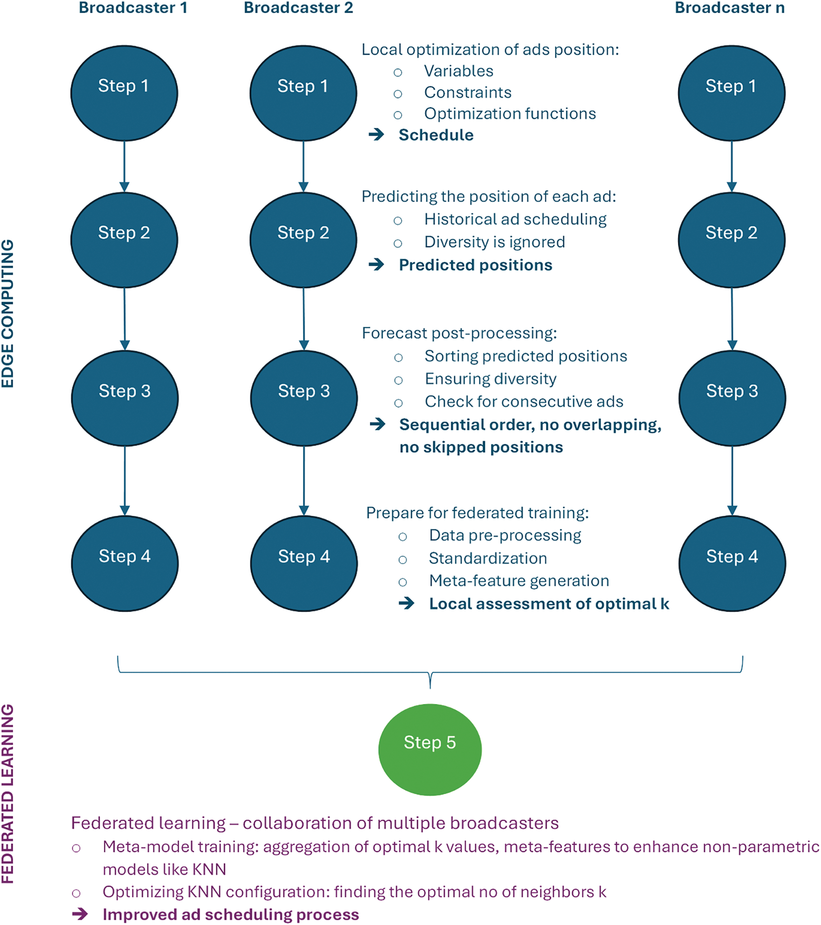
Figure 1: Process flow diagram

3.1 Input Data

The dataset at each station includes: AdName—the name or identifier of the advertisement; AdCost—the cost associated with airing the advertisement; Category—the category of the product or service being advertised; Length—the duration of the ad in seconds; BreakId—a unique identifier for each ad break; TV Show Name—the name of the TV show during which the ad break occurs; BreakInd—a unique index or identifier for each break instance in the datasets; AdCost_first—the cost of the ad positioned first within the break; AdCost_second—the cost of the ad placed second in the break; AdCost_bef_last—represents the cost of the ad scheduled before the last position; AdCost_last—the cost of the ad positioned last within the break. For a particular break, the dataset is provided in Table 2.

3.2 Optimization Process

To formulate this as an optimization problem, we define the decision variables, constraints and objective functions as follows:

•   Decision variables

xijk: Binary variable that equals 1 if ad k is placed in position j during break i, and 0 otherwise.

Li: Length of break i.

pjk: Bidding price for ad k in position j.

Di: Diversity score for break i.

This binary variable xijk is crucial for determining the placement of ads. It defines whether an ad k is placed in position j during break i. The indexes i, j and k correspond to the break, position within the break and specific ad, respectively. Li represents the length of each break i. This is a given parameter rather than a decision variable and should be corrected in the initial explanation. pjk is the bidding price for placing ad k in position j. These are parameters determined by the advertisers’ bids and are important for calculating revenue. Di is diversity score for each break i, which needs to be calculated based on the variety of ad categories within a break.

•   Parameters

N: Total number of breaks.

Mi: Number of ads per break i.

Ck: Category of ad k.

Lk: Length of ad k.

Bi: Total length available in break i.

Lk and Bi are given parameters specifying the length of each ad and the total length available for ads in each break, respectively. Each ad k belongs to a specific category Ck, which is important for calculating diversity.

•   Constraints

Ad placement uniqueness. Ensures that each position in a break is filled by exactly one ad and that an ad does not appear more than once in the same break. This maintains the integrity of ad scheduling. Each position can only be filled by one ad and each ad can only appear once in a break.

∑kxijk=1,∀i,j(1)

∑jxijk≤1,∀i,k(2)

Length constraint. The total length of ads should not exceed the length of the break. Guarantees that the combined length of all ads in a break does not exceed the total available duration of that break. This constraint is fundamental to avoid overbooking the break time.

∑j∑kLk×xijk≤Bi,∀i(3)

Diversity constraint. Implement a scoring system to ensure diversity in ad categories within a break. This involves calculating the number of unique categories per break and ensuring it meets a predefined threshold Divthr or more complex scoring based on the distribution of categories. It aims to maintain a diverse range of ad categories within each break. The diversity score Di could be calculated using various methods, such as the number of unique categories present. This ensures that viewers are exposed to a variety of ads, which enhance viewer engagement and satisfaction.

Di≥Divthr,∀i(4)

Value maximization constraint. Ensure the highest-value ads are placed in the first or last position. This constraint requires a dynamic definition based on the bidding prices for the first and last positions. Prioritizes placing the highest bidding ads in the most valuable positions (first or last) within a break. This constraint is designed to maximize revenue by leveraging the bidding prices associated with these prime positions.

p1k≥pjk,∀j≠1,kfor the first position(5)

pMik≥pjk,∀j≠Mi,kfor the last position

Bidding price sequence constraint. This implicitly affects how the optimization algorithm will prioritize placing ads based on the bidding price for each position. This constraint outlines the expected order of bidding prices from highest to lowest based on ad positions. It ensures that the ad placement aligns with the bidding strategy, placing higher value on the first and last positions and subsequently for the second and the one before last positions.

p1k≥pMik≥p2k≥p(Mi−1)k≥pjk,∀j∉{1,2,Mi−1,Mi},k(6)

•   Objective function

The objective is to maximize both the revenue and the diversity score. This is a multi-objective optimization problem or a weighted sum of both objectives. Assuming ω1 and ω2 are the weights for revenue and diversity, respectively, the objective function can be formulated as:

MaximizeZ=ω1×(∑i∑j∑kpjk×xijk)+ω2×(∑iDi)(7)

where ω1+ω2=1.

This formulation allows for the balancing of revenue generation with the goal of maintaining diversity within ad breaks. Adjusting the weights ω1 and ω2 can prioritize one objective over the other based on the broadcaster’s strategy. The diversity score Di for each break can be calculated based on the diversity of categories present, with higher scores indicating greater diversity. This could involve complex calculations outside the scope of linear programming and might require heuristic or algorithmic approaches to estimate effectively.

The objective function combines revenue maximization with diversity enhancement. It is formulated as a weighted sum to allow for flexibility in prioritizing these objectives:

•   the revenue part of the objective ω1×(∑i∑j∑kpjk×xijk) calculates the total revenue from ad placements, where ω1 is the weight representing the importance of revenue.

•   the diversity part ω2×(∑iDi) adds the diversity scores of all breaks, weighted by ω2, which reflects the importance of maintaining diversity within ad placements.

The weights ω1 and ω2 allow for customization based on the broadcaster’s strategic priorities. For instance, if revenue maximization is paramount, ω1 could be set higher than ω2. Conversely, if ad diversity is more critical, ω2 would be increased. These weights must sum to 1 to ensure that the objective function remains normalized.

3.3 KNN and Other Prediction Models

Essentially, KNN uses the distances between data points to make predictions or decisions without making assumptions about the distribution of the underlying data. The first step in KNN is to calculate the distance between the new point and all existing points in the training set. Although Euclidean distance is the most common choice, other values such as Manhattan (L1 norm) Minkowski and Hamming distance can be used. The choice of distance metric can influence the performance of the algorithm. Choosing K (the number of nearest neighbors to consider) is the most important step. A small K makes the model sensitive to noise, while a large K makes it computationally expensive and possibly over-smoothed. There is no universal value for K and it is usually chosen by cross-validation. Once the distances between the points are calculated and the closest ones K neighbors are identified, the algorithm aggregates their labels. In classification problems, the most common label among those K nearest neighbors is assigned to the new data point. For example, if K = 5 and three neighbors belong to Class A and two belong to Class B, the new data point will be assigned to Class A. For regression problems, the algorithm predicts the value for the new point based on the average or weighted average of the values of its K nearest neighbors.

Considering extensive datasets and the multifaceted challenges introduced by high-dimensional spaces, the efficacy and computational efficiency of KNN can be significantly hindered, therefore we also explored other solutions, such as Light Gradient Boosting Machine (LightGBM) and Random Forest. The LightGBM is a gradient boosting algorithm designed by Microsoft, which utilizes tree-based learning algorithms. Unlike traditional gradient boosting methods that grow trees level-wise, LightGBM grows trees leaf-wise, which results in much faster learning speeds. LightGBM is a gradient boosting framework that uses tree-based learning algorithms [36]. It is designed for distributed and efficient training, especially on large datasets and it can handle large amounts of data easily. It is often implemented for its speed and performance, as well as its ability to manage categorical features. Random Forest is an ensemble learning method that operates by constructing a multitude of decision trees during training time and outputting the mean prediction of the individual trees [37]. Random Forests create an ensemble of Decision Trees using bootstrapped datasets, which means random samples with replacement from the original dataset.

3.4 Post-Processing Step in KNN

The proposed post-processing step is significant as it processes the results of KNN prediction and assigns a position of the ad by sorting out the results. Furthermore, it ensures that the sequence of the ads offers the required diversity for advertisers by implementing a consistent check condition. The post-processing step allows for the integration of these important business rules and constraints, refining the initial KNN output to meet operational requirements.

For each ad break (identified by BreakId), we first sort the ads based on their initially predicted positions (prediction column). This step organizes ads in the sequence determined by the predictive model, setting the foundation for subsequent adjustments. Then, we calculate a new sequence of positions, starting from 1 up to the number of ads in the break. This recalculated sequence ensures that every ad is assigned a unique and sequentially ordered position, addressing potential issues of overlapping or skipped positions in the initial predictions. Within each sorted break, we identify the ad with the lowest cost (AdCost). The lowest-priced ad is then assigned a position in the middle of the sequence. Following the strategic placement of the lowest-priced ad, we adjust the positions of the remaining ads to maintain a logical sequence. Each ad is sequentially ordered, ensuring no gaps or overlaps in positions.

Another aspect of the post-processing method is ensuring diversity in ad categories within each break. Therefore, we implement a check for consecutive ads from the same category and adjust positions to prevent this, aiming to maintain viewer engagement by offering varied content.

3.5 Federated Learning

In many industries, such as healthcare, finance and advertising, data privacy regulations and concerns prevent the pooling of data into a central repository. FL offers a solution by enabling models to learn from decentralized data sources without the data ever leaving its original location. FL offers a compelling solution to this challenge. By allowing multiple broadcasters to collaborate and improve their ad scheduling models without directly sharing sensitive data, FL fosters a privacy-preserving, collective intelligence approach. Datasets across different clients (e.g., hospitals, banks, advertising stations) often vary not just in size, but in feature space and distribution. This heterogeneity makes it challenging to apply a one-size-fits-all model or to directly aggregate model parameters as in traditional FL approaches. On the other side, KNN is a non-parametric algorithm that relies on the local dataset for making predictions. Unlike parametric models, KNN does not have a fixed set of parameters that can be easily averaged across clients. This poses a challenge for optimizing KNN in a federated setting, where direct data access or aggregation is not feasible. The optimal configuration for a KNN model (e.g., the number of neighbors, K) may significantly vary depending on the specific characteristics of a dataset. Finding an optimal K that suits the local data of each client is the problem that we will solve.

The flow description includes:

1) Data preprocessing and standardization. This step ensures that all clients process their data in a consistent manner, facilitating more meaningful comparisons and aggregations despite data heterogeneity;

2) Meta-feature generation. By extracting meta-features that describe each client’s dataset, the approach abstracts dataset characteristics in a way that can be shared without compromising data privacy, enabling the central server to gain insights into the data landscape across clients;

3) Local evaluation for optimal K. It allows each client to independently determine the K value that best suits their data, ensuring that local model configurations are tailored to maximize performance given the local data characteristics;

4) Meta-model training. The central aggregation of optimal K values and corresponding meta-features to train a meta-model introduces a novel way to optimize non-parametric models like KNN in a FL framework. This meta-model predicts the optimal K for any client based on its dataset’s meta-features, guiding the local configuration of KNN models across the network.

Step 1. Data preprocessing and standardization

For each client i with dataset Di, the preprocessing function fp is applied to transform the dataset into Di′: Di′ = fp(Di) where Di′ includes standardized numeric features, encoded categorical features and imputed or placeholder values for missing data. Each client implements two pipelines: a numeric transformer and a categorical transformer. For the numeric transformer pipeline, missing values are filled with the column mean and StandardScaler in Python is applied to normalize the numeric features, ensuring they have a mean of 0 and a standard deviation of 1. For the categorical transformer pipeline, missing values in categorical columns are filled with a placeholder value (‘missing’) and OneHotEncoder converts categorical variables into a set of binary variables (0 and 1 s), one for each category. The results from the two pipelines are combined using a ColumnTransformer. This step applies the appropriate transformations to each column in the DataFrame for each client based on its type (numeric or categorical). The target variable—Scheduled_Position, is excluded from features before transformation to avoid altering the target variable. The preprocessor is then applied to the dataset’s features, executing the defined transformations.

Step 2. Meta-feature generation

Given the preprocessed dataset Di′, a meta-feature vector Mi is generated to describe the dataset’s characteristics:

Mi=g(Di)(8)

where g is a function that extracts meta-features such as the number of features, mean, variance, unique categories and binary indicators for special features or constraints.

Step 3. Optimal K local evaluation

Each client evaluates a range of K values to find the optimal Kiopt based on a performance metric P through cross-validation:

Kiopt=argmaxP(K,Di′)(9)

Step 4. Meta-model training

Aggregating meta-features Mi and optimal Kiopt values from all clients, a central dataset (Xmeta, Ymeta) is formed for the meta-model training:

Xmeta={M1,M2,…,Mn},Ymeta={K1opt,K2opt,…,Knopt}(10)

The meta-model Mmeta is trained to predict the optimal K based on meta-features:

Mmeta:Xmeta→ymeta(11)

For a new or existing client with dataset Dj′ and meta-features Mj, the meta-model predicts the optimal:

Kjopt:Kjopt=Mmeta(Mj)(12)

Each client uses historical ad scheduling data, including features such as ad cost, length, category and previously determined optimal positions, to train their local KNN model. The goal is to predict the most effective ad positions, applying a post-processing step to adjust predictions based on strategic considerations and operational constraints specific to each station. For each client the first step is to prepare the dataset before generating meta-features. The preprocessing includes encoding categorical variables, scaling numeric features and handling missing data.

Regarding implementation, encryption is the first line of defense in securing the model updates and meta-features generated by each client. At its core, encryption involves converting plaintext data into ciphertext, a coded format that is unintelligible without the correct decryption key. This process ensures that even if the data is intercepted during transmission, it cannot be deciphered by unauthorized parties.

In symmetric encryption, the same key is used for both encryption and decryption. This method is computationally efficient, making it suitable for encrypting large amounts of data quickly. However, the challenge lies in securely sharing the key between the sender and the receiver, as the key itself must be protected during transmission. On the other hand, asymmetric encryption uses a pair of keys, a public key for encryption and a private key for decryption. The public key can be openly shared, while the private key remains confidential. This method is more secure for key exchange but is computationally more intensive than symmetric encryption. It is commonly used in establishing secure channels before switching to symmetric encryption for the actual data transmission. In the context of FL, asymmetric encryption is often used during the initial setup to securely exchange a symmetric key, which is then used to encrypt the model updates. This hybrid approach leverages the strengths of both encryption methods: the security of asymmetric encryption for key exchange and the efficiency of symmetric encryption for data transmission.

Once the data is encrypted, it must be transmitted over the network in a way that prevents unauthorized access and tampering. Secure transmission protocols are designed to ensure the confidentiality, integrity, and authenticity of the data in transit.

Secure Sockets Layer/Transport Layer Security (SSL/TLS) and its successor are cryptographic protocols that provide secure communication over a computer network. These protocols use asymmetric encryption to establish a secure connection, followed by symmetric encryption for the data exchange. TLS is the more modern and secure version, addressing several vulnerabilities found in SSL. The TLS handshake is the initial phase where the client and server authenticate each other and agree on the encryption methods to use. This process involves the exchange of certificates and cryptographic keys. The handshake establishes a secure session before any actual data is transmitted.

A few key problems and challenges can be tackled in the context of secure transmissions in an FL system. As the number of clients in a FL system grows, the complexity of managing secure transmissions increases. Each new client adds to the computational and network load, which can lead to bottlenecks. After securely transmitting the encrypted model updates and meta-features from each client to the central server, the next step in the process is the aggregation of these updates to form a global model. This aggregation phase is where the decentralized insights from individual clients are combined, allowing the global model to generalize across the diverse datasets distributed among the clients. Aggregation in FL involves the process of consolidating the model updates received from multiple clients into a single, cohesive global model. This is particularly important in FL because each client operates on a unique, often non-IID (independent and identically distributed) dataset, leading to model updates that reflect different aspects of the underlying data distributions. At its core, the aggregation method needs to ensure that the global model benefits from the collective intelligence of all participating clients while respecting the privacy and independence of their data. In typical scenarios, such as with deep neural networks, this aggregation involves averaging the weights of the models trained on each client’s data. However, with non-parametric models like KNN, the approach to aggregation must be adapted to handle the instance-based nature of these models.

During local model training, each client computes meta-features that summarize important characteristics of its dataset and model performance. These include statistical measures like mean, median, and standard deviation of prices within the top n predictions, the diversity of ad categories and average user engagement scores. When implementing this in code, each client would store these meta-features in a structured format, such as a dictionary or a custom object, before encrypting and transmitting them to the server. At the central server, the received meta-features from all clients are decrypted and then aggregated. Once trained, this meta-model is used to recommend the best K value for each client based on their meta-features, ensuring that each KNN model is optimally configured. Since each client’s dataset can be vastly different in terms of distribution and size, the aggregated meta-features and K values do not reflect a one-size-fits-all solution. A weighted aggregation approach, where clients with more representative or higher-quality data have more influence, mitigates this issue. For many features like num_samples, price_mean, and spot_length_mean, simple averaging across clients can provide a meaningful central tendency that represents the typical characteristics of the datasets. For instance, averaging price_mean across all clients gives the central server an idea of the general pricing trend across different datasets. In cases where clients have significantly different dataset sizes or data quality, a weighted aggregation can be more appropriate. In this case, each client’s meta-features are weighted by factors such as the number of samples (num_samples) before aggregation. This ensures that clients with more representative or larger datasets have a proportionally greater influence on the global meta-features. The aggregated meta-features are then used as input to a meta-model, which is a higher-level predictive model designed to optimize certain hyperparameters across the network, such as the optimal K. The meta-model uses the aggregated features like category_id_mean, position_mean, and price_var to learn how these characteristics impact the effectiveness of ad placements. For example, position_var might indicate how consistently ads are placed within certain slots, which can correlate with viewer engagement or pricing strategies.

Using ML techniques such as Random Forest or Gradient Boosting, the meta-model analyzes the relationships between the aggregated meta-features and the optimal K values previously reported by the clients. By learning from these historical patterns, the meta-model predicts the most suitable K for new or existing clients based on their current meta-features. For instance, if a dataset has a high price_var coupled with a low position_var, the meta-model might infer that a slightly higher K is optimal to account for the stable ad positions but variable pricing.

In a FL environment, straggler nodes are clients that, due to slower computational resources, network latency or larger datasets lag other clients in completing their tasks, such as training local models or generating meta-features. One common approach to dealing with straggler nodes is implementing asynchronous aggregation. In this setup, the central server does not wait for all clients to finish their updates before proceeding with the aggregation and model update. Instead, the server aggregates the updates from the clients that have completed their tasks and proceeds to update the global model. As each client completes its model training and meta-feature generation, it sends its update to the server. The server continuously aggregates these updates, allowing faster clients to contribute without waiting for the slower ones. This approach ensures that the global model is updated regularly, even if some clients are still processing. Asynchronous aggregation reduces the overall time required to update the global model, improves system throughput and makes the FL process more resilient to network delays or varying computational capabilities among clients.

Partial participation is another technique where, in each round of FL, only a subset of clients is selected to participate in the training process. This selection can be randomized or based on certain criteria, such as the client’s historical performance or current computational capacity. The central server may randomly select a percentage of clients to participate in each round. This reduces the waiting time for slower clients and also mitigates the impact of stragglers by not requiring every client to contribute to every round. This approach reduces the overall computational load on the server and clients, while still ensuring that over time, all clients contribute to the global model. It also helps balance the contribution of clients with varying capabilities and resources.

Dynamic timeouts involve setting a maximum time limit for clients to complete their tasks and send their updates. Clients that exceed this time limit are excluded from the current aggregation round but can participate in future rounds. The server sets a dynamic timeout based on the observed performance of clients. For instance, if most clients typically complete their tasks within a certain time frame, the server sets a timeout slightly above this average. Clients that fail to submit their updates within this time are considered stragglers and are bypassed in that round. This method ensures that the global model updates are not unduly delayed by a few slow clients. It also provides a safeguard against network issues or unexpected delays that might affect client performance. To further assist straggler nodes, the system may implement checkpointing, where clients periodically save their progress during training. If a client is identified as a straggler and cannot complete its task in time, it can resume from the last checkpoint in the next round rather than starting from scratch. Clients save their model state and meta-features at regular intervals. If a client is unable to complete its work within the allotted time, it can resume from the last saved state in the subsequent round. This reduces the overall time required for training and allows stragglers to catch up more efficiently. Checkpointing reduces the computational burden on straggler nodes and prevents the loss of progress, ensuring that even slower clients can eventually contribute to the global model.

4  Results

4.1 Optimization

Google’s OR-Tools is a robust suite designed to tackle a broad spectrum of optimization challenges, including but not limited to routing, scheduling and comprehensive planning tasks. In the context of multiple objectives, OR-Tools adeptly navigates through the complexity of optimizing a primary goal while simultaneously respecting the bounds of secondary objectives. This is achieved through various methodologies such as the weighted sum approach, lexicographic ordering or goal programming, each providing a nuanced strategy to balance and satisfy the array of objectives inherent in complex problems. The suite is equipped to handle many constraint types including linear, integer and network flow constraints, among others. This capability was considered also when the tool was chosen for solving the depicted optimization problem.

Our model comprises n ads, each with a predefined category and price. We define a set of integer variables, ad_positions[i], for i = 1,...,n, representing the position of each ad within the commercial break. The domain of these variables is constrained between 0 and n−1, inclusive, ensuring a valid positioning within the break. To address our objective of placing the highest-priced ad either at the beginning or end of the sequence, we first identify the maximum price, max_price, from the provided data. We then construct a linear expression summing the positions of all ads priced at max_price and constrain this sum to take on values corresponding to the start or end positions only. Additionally, to avoid consecutive ads from the same category (thus promoting variety), we introduce binary variables, same_cat_next[i], for i = 1,...,n–1, that activate when consecutive ads share the same category. The constraint model.AddBoolOr([same_cat_next[i].Not()]) ensures no two consecutive ads share the same category, enhancing the viewer’s experience by diversifying the content.

The implementation utilizes the CP-SAT solver for solving constraint programming models. The solver attempts to find an optimal solution that respects all defined constraints, including the all-different constraint for ad positions, the placement of the highest-priced ad and the avoidance of consecutive ads from the same category. Upon solving, the model retrieves the optimal or feasible sequence of ads, displaying each ad’s position, price, and category.

For a given entry of the dataset:

Data = {

‘spot’: [‘Spot 1’, ‘Spot 2’, ‘Spot 3’, ‘Spot 4’, ‘Spot 5’, ‘Spot 6’, ‘Spot 7’, ‘Spot 8’],

‘category’: [‘Cat A’, ‘Cat B’, ‘Cat C’, ‘Cat C’, ‘Cat C’, ‘Cat D’, ‘Cat E’, ‘Cat F’],

‘price’: [140.1,152.11,138.2,105.4,161.11,161.13,161.11,258.11]

}

The output is as follows:

Ad sequence:

(‘Spot 8’, 258.11, ‘Cat F’)

(‘Spot 1’, 140.1, ‘Cat A’)

(‘Spot 7’, 161.11, ‘Cat E’)

(‘Spot 3’, 138.2, ‘Cat C’)

(‘Spot 2’, 152.11, ‘Cat B’)

(‘Spot 5’, 161.11, ‘Cat C’)

(‘Spot 6’, 161.13, ‘Cat D’)

(‘Spot 4’, 105.4, ‘Cat C’)

The dataset will now have a new feature “ScheduledPosition” which will be populated with the determined position from the optimization algorithm. The dataset used for training at an individual TV post level consists of 93,941 entries records of spots with corresponding scheduled positions, the total price and the price for first, second last and before last positions inside the break.

The following plots provide a comprehensive analysis of ad scheduling across multiple breaks, focusing on the distribution of ad positions, break durations and category assignments.

Fig. 2: displays the distribution of scheduled ad positions across multiple breaks, with positions numbered from 1 to 42. The x-axis represents the ad positions within a break, while the y-axis shows the count of ads scheduled at each position. By Position 20, the number of scheduled ads drops below 1000 and positions beyond 25 see very few ads scheduled.

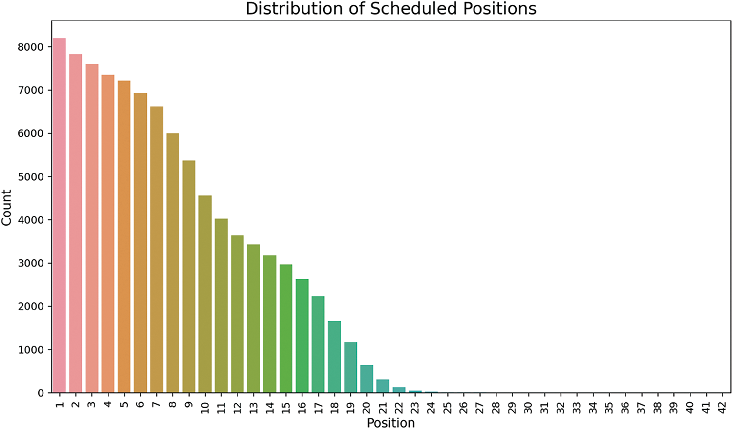
Figure 2: Distribution of scheduled ad positions

Fig. 3 visualizes the relationship between ad positions and total break duration. The x-axis represents the total break duration in seconds, while the y-axis represents the ad positions. The darker blue regions indicate higher densities, meaning more occurrences of ads scheduled at those positions and break durations. The second, more prominent cluster, appears around 400 s of break duration and covers ad positions from 10 to 20. This suggests that as the total break duration increases, ads tend to be more evenly distributed across middle positions. Notably, beyond 500 s, the density diminishes significantly, indicating that very long breaks are less common and fewer ads are scheduled in those breaks.

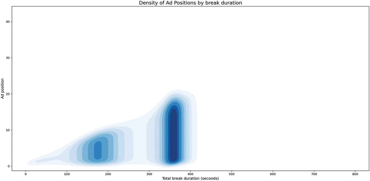
Figure 3: Density of ad positions by break duration

The steady upward trajectory in Fig. 4 shows a clear linear pattern until around 500 s of total break duration, after which the mean ad position continues to rise but with more variance. The sharp increase beyond 600 s indicates that in very long breaks, ads are typically placed toward the end of the slot, reflecting that these breaks have more available positions and less emphasis on front-loading the ads.

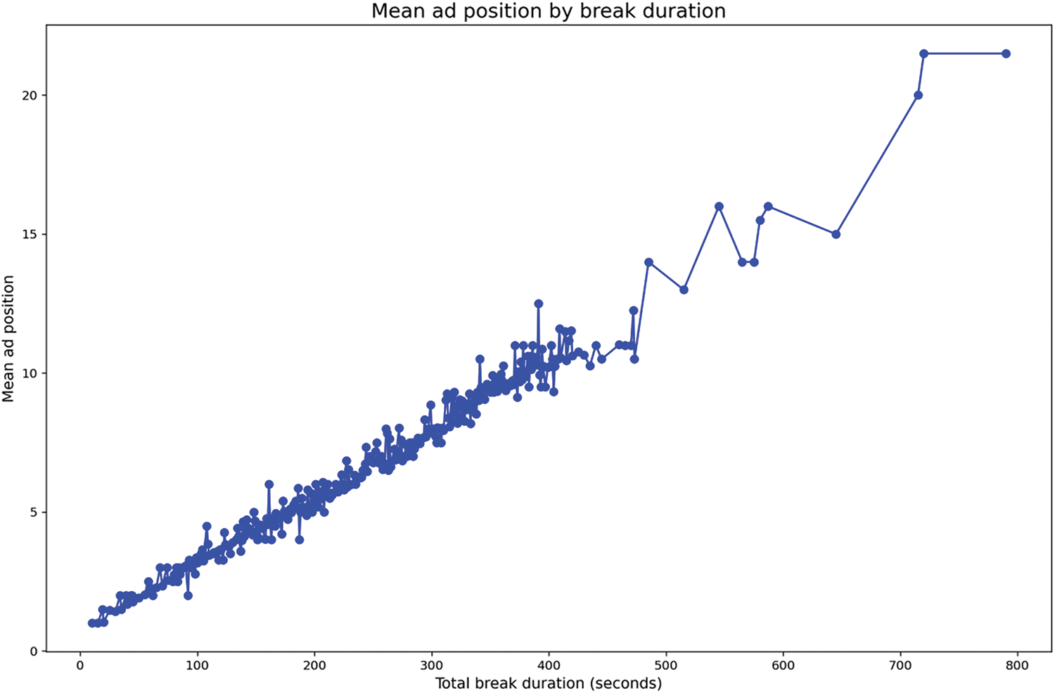
Figure 4: Mean ad position by break duration

Fig. 5 presents the distribution of advertisement categories across 10 breaks, with each row representing one break and the scheduled positions shown along the x-axis. The categories, such as Analgesic, Medical Device, Food Supplement and Supermarkets, are assigned to specific positions within each break. The heatmap captures the original category distribution as observed in the data, with Analgesic appearing more frequently across multiple positions and breaks. This provides a clear representation of how categories were originally distributed across different breaks in the dataset.

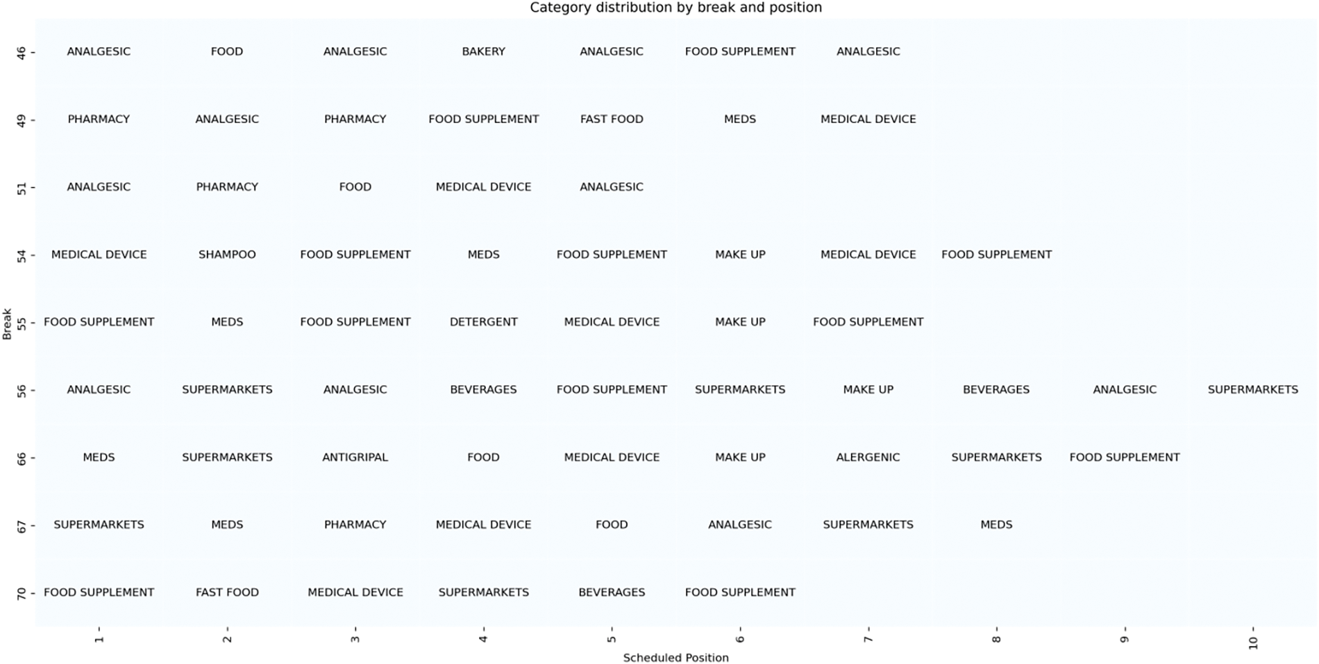
Figure 5: Ad categories across ten breaks

Fig. 6 illustrates the ad position distribution per break, with each row corresponding to a specific break and each column representing a scheduled position (1 to 10). The intensity of the color reflects the duration of ads in seconds, with darker shades indicating longer ad durations.

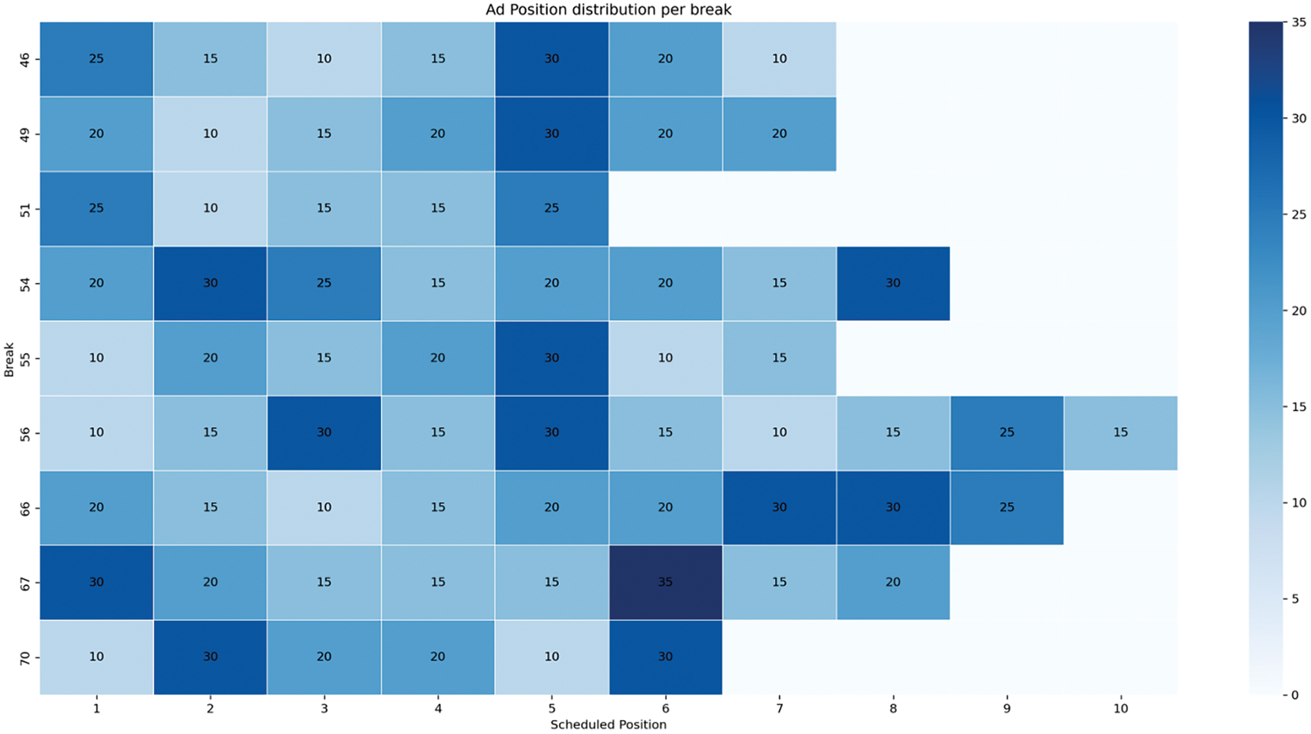
Figure 6: Ad position distribution for ten breaks

4.2 KNN Implementation

The set of features (X) includes various cost-related attributes of ads (AdCost and specific positional costs like AdCost_first, AdCost_second, etc.), which influence their optimal scheduling positions. The target variable (y) is the SchedulePosition, indicating where each ad should ideally be placed within a break. The dataset is divided into training and testing sets using train_test_split, with 80% of the data allocated for training and 20% for testing. This split facilitates model training on one subset of the data and unbiased evaluation on another.

Since KNN calculates distances between data points, feature scaling is essential to ensure that all features contribute equally to the distance computations. The StandardScaler normalizes features, so they have a mean of 0 and a standard deviation of 1, preventing features with larger scales from dominating the distance calculations.

A 10-fold KFold cross-validation approach is used to assess model performance, ensuring robustness and generalizability across different subsets of the data. The model is then tested on the test set shaped of (28183, 15) to evaluate the predictive accuracy.

For a better understanding of the algorithm results, we plot the number of identical results by comparing the actual number of values where the determined position is equal to the predicted one (as in Fig. 7), and for the rest we plot the results based on the difference between the actual result and the predicted value. Therefore, on the x-axis, we will have categories for “Identical Values” and various ranges of differences (e.g., 0–1, 1–2, 2–3, 3–4 and greater than 5). The y-axis will show the count of occurrences in each category. The usage of accuracy as the evaluation metric stems from its alignment with the core business objectives of ad scheduling. The task is to predict the optimal ad positions within an ad break, where specific positions (such as first and last) carry higher revenue potential and viewer engagement. Given that the placement of ads directly impacts revenue, accuracy, defined here as the exact match between predicted and actual positions, serves as a practical and business-relevant measure of performance. For instance, after post-processing the KNN model’s predictions, approximately 8400 exact matches were achieved, indicating that the model effectively predicted the correct ad positions. In this sense, accuracy provides a clear and interpretable metric that reflects the model’s ability to meet revenue optimization goals. Thus, in contexts where exact placement can have significant financial implications, such as TV advertising, accuracy becomes a suitable and intuitive measure of success. This research evaluates the model by categorizing prediction errors into ranges like “0–1”, “1–2”, and “greater than 5”. This granularity allows to quickly grasp how often predictions fall within an acceptable range, and how many times the predictions were exact, as visualized in Figs. 7 and 8. This practical focus ensures that the accuracy metric remains closely aligned with real-world objectives, making it an effective choice for evaluation. The post-processing improves the predictions, refining the model to meet real-world scheduling needs, such as maintaining category diversity, which are essential for viewer engagement. By measuring how well the model performs after this optimization, accuracy captures the effectiveness of the entire process, not just the raw predictions. This combination of optimization and prediction enhances the system’s overall performance, making accuracy a fitting metric to evaluate the success of the model in both the technical and business domains. When comparing multiple models (e.g., KNN vs. Random Forest vs. LightGBM), accuracy provides a common, simple metric to benchmark how well each model performs in terms of exact position matches. This simplicity allows for clear comparisons of model performance across different algorithms. Since the predicted positions are rounded to integers, accuracy becomes a natural fit for evaluation. While other regression metrics like MAE or MSE could capture the magnitude of the error, accuracy focuses on how well the model performs after rounding, which reflects the final, real-world outcome of the predictions.

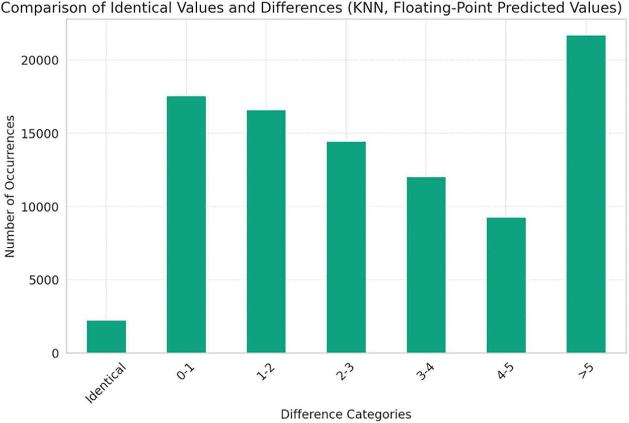
Figure 7: Comparison of identical values and differences (KNN, floating point predicted values)

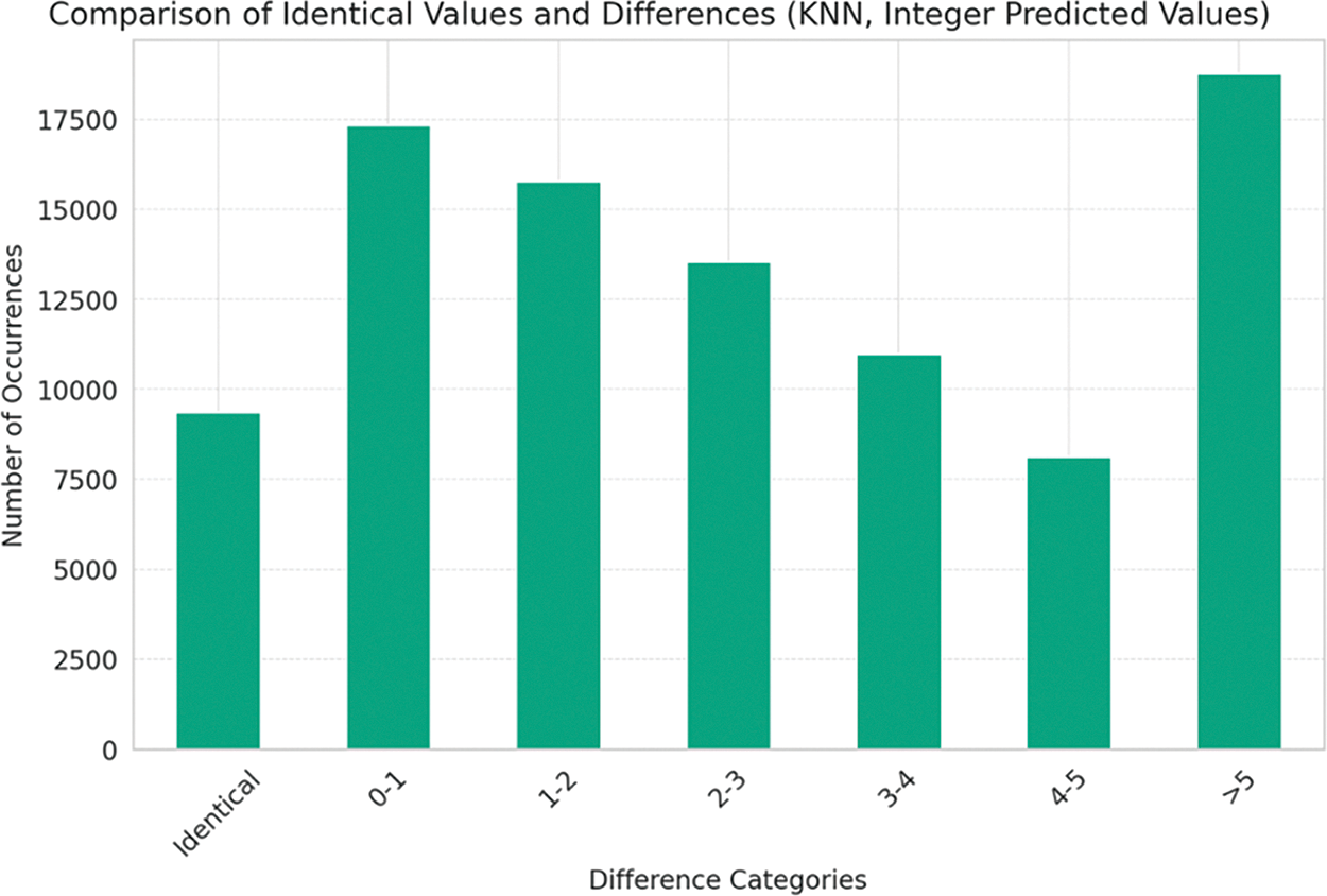
Figure 8: Comparison of identical values and differences (KNN, integer predicted values)

Fig. 8 shows the differences between the actual position of the spots and the predicted outcomes, after the predicted outcome was converted to an integer value.

KNN predictions provide a raw ordering based on historical data and feature similarity. However, these predictions might not fully align with practical scheduling needs, such as avoiding ad content repetition or ensuring diversity in ad categories.

Furthermore, Random Forest and LightGMB are applied to the dataset and results are evaluated on 20% of data. Random Forest is an ensemble learning method that operates by constructing a multitude of decision trees during training time and outputting the mean prediction of the individual trees. Random Forests create an ensemble of Decision Trees using bootstrapped datasets, which means random samples with replacement from the original dataset. LightGBM is a gradient boosting framework that uses tree-based learning algorithms. It is designed for distributed and efficient training, especially on large datasets, and it can handle large amounts of data with ease. It is often praised for its speed and performance, as well as its ability to manage categorical features.

For evaluating the algorithms (RF, LGBM, KNN) results, the Figs. 9 and 10 show on the x-axis categories of differences between the actual and predicted values, labeled as ‘Identical’, ‘0–1’, ‘1–2’, ‘2–3’, ‘4–5’, and ‘>5’, indicating the range of error.

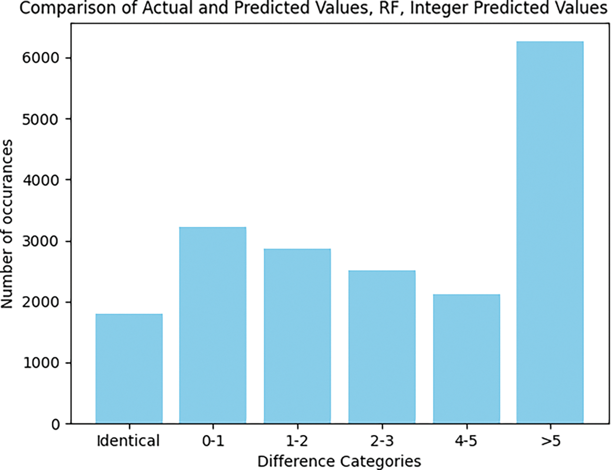
Figure 9: Comparison of identical values and differences (RF, integer predicted values)

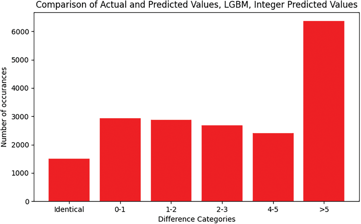
Figure 10: Comparison of identical values and differences (LGBM, integer predicted values)

The y-axis shows the number of occurrences, or how often predictions fell within each error category. Each bar’s height corresponds to the number of instances where the predicted value was within the specific error range relative to the actual value. By comparing the bars, especially those labeled ‘Identical’ and ‘0–1’, we may sense of how often each model accurately predicts the positions variable, considering that an extra processing step was made—the predicted positions were rounded to the closest integer value. More occurrences in these categories typically indicate better performance. The bars labeled ‘>5’ are particularly telling, as they represent instances where the model’s predictions were off by more than 5 units from the actual value. A higher bar in this category would indicate less accuracy.

Further, we seek to enhance the predictive accuracy of ad spot placement by incorporating a new feature into the model. While KNN served as the primary algorithm, we introduce an interaction feature to capture more complex relationships between the existing variables. Specifically, we generated the new feature by multiplying the ad price with the square of the scheduled position column: df[‘interaction_feature’] = df[‘price’] x (df[‘pos’]^2). This interaction feature aims to better represent how ad pricing interacts with the positioning of ads in a more non-linear manner, allowing the model to learn from these interactions more effectively. By squaring the scheduled position and multiplying it by the price, the feature emphasizes the importance of both variables in influencing ad spot placement, particularly for higher-priced ads in more critical spots.

The results shown in Fig. 11 depict the distribution of differences between the predicted and actual values for ad spot placements using the KNN model. Most predictions fall under the “Identical” category, indicating that the model accurately predicted the exact spot placements in most cases, with over 35,000 instances showing no difference between predicted and actual values. This highlights the high accuracy of the KNN model in this experiment.

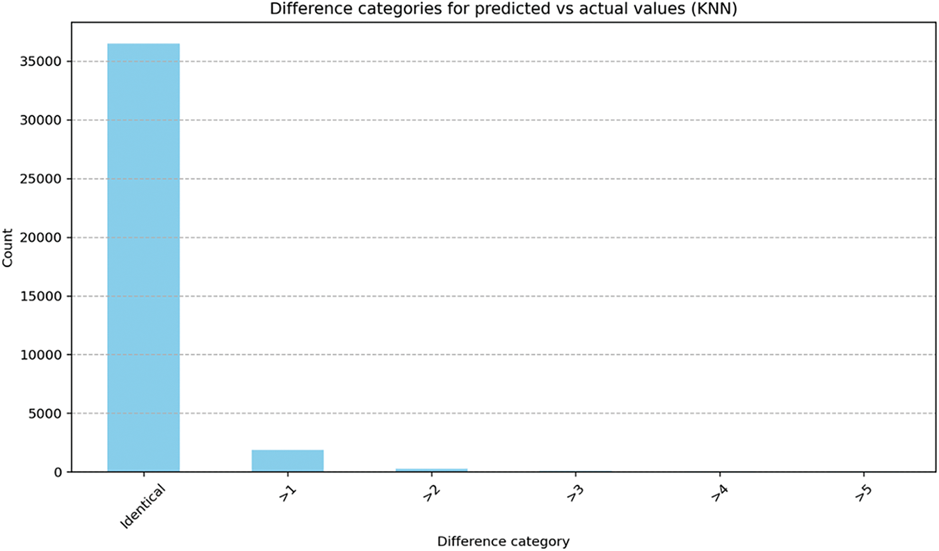
Figure 11: Difference categories after adding a new feature

However, there are also a few instances where the predicted spot differs from the actual value, with a small number of cases in the “>1” difference category. These deviations suggest that while the model performs well overall, there are certain cases where the ad spot prediction may not align perfectly, due to limitations in capturing the complexity of some ad scheduling patterns.

Overall, this result reinforces the strength of the KNN model, especially after introducing the interaction feature (which helped improve prediction accuracy, as evidenced by the overwhelming number of identical predictions). While the introduction of the interaction feature significantly improved the model’s accuracy by capturing complex relationships between price and ad spot position, it also introduces certain disadvantages. One primary drawback is the potential for overfitting. The squared term in the interaction feature may cause the model to be too sensitive to extreme values, leading it to fit noise or outliers in the training data, rather than generalizing well to new data. This could explain why a small number of predictions fell outside the “Identical” category in the results, where the model may have struggled with more variable or less predictable ad placements. Another limitation is the added complexity to the model, which can impact interpretability. While the interaction feature boosts performance by modeling non-linear relationships, it makes the model more difficult to interpret, particularly for stakeholders who might rely on clear insights into why specific ads are placed in certain spots. Additionally, this interaction feature may have limited applicability across different datasets or contexts. The specific relationship between price and scheduled position captured by squaring the scheduled position might not hold true in other scenarios, limiting the generalizability of the model.

4.3 Post-Processing Step in KNN

After post-processing the differences between actual positions and predicted ones are presented in Fig. 12.

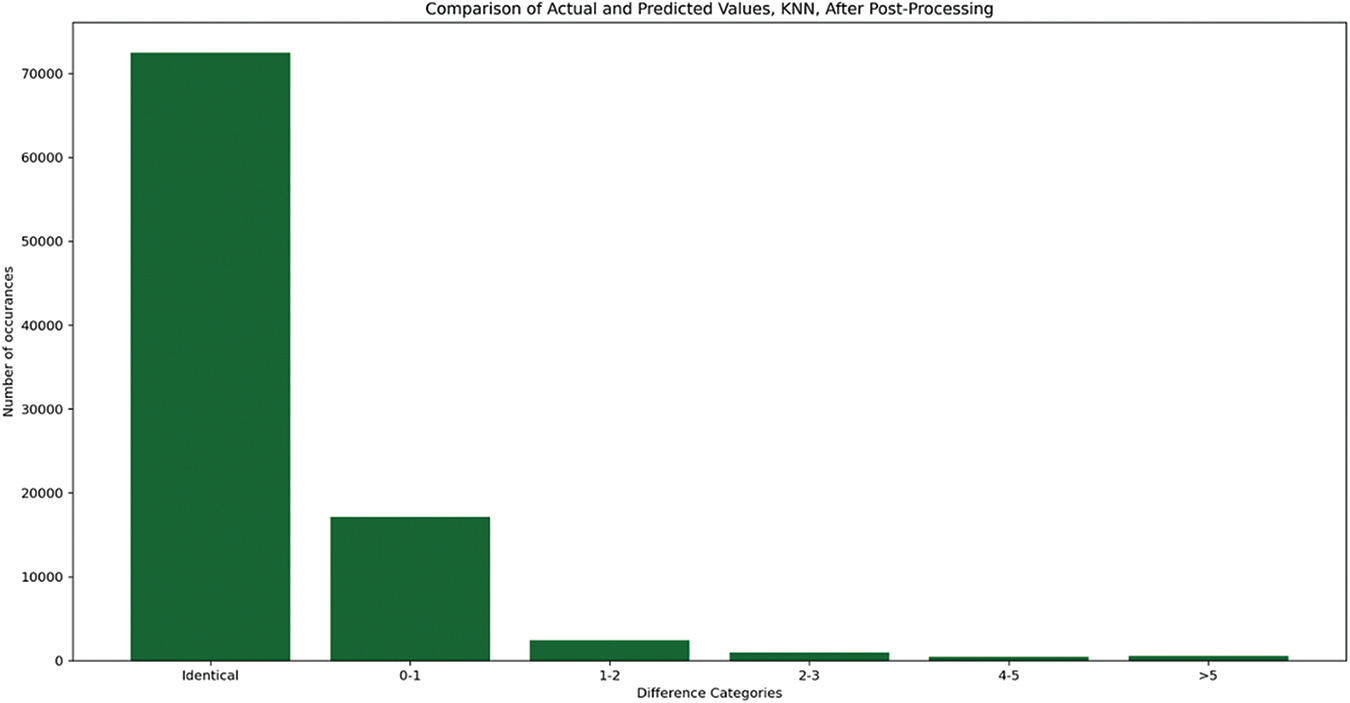
Figure 12: Comparison of identical values and differences after post-processing

This plot indicates the performance of the proposed method that combines optimization, prediction and apost-processing step.

4.4 Federated Learning

The primary objective of the simulation is to optimize the scheduling of TV advertisements for a specific TV post by leveraging constraint programming. The optimization criteria included maximizing ad price visibility and ensuring category diversity within each ad break, aiming to increase viewer engagement and advertising revenue. The optimization model defines several constraints, such as: each ad is assigned a unique position within an ad break; ads with the highest price are preferentially placed at the beginning or end of the break, maximizing their visibility and consecutive ads must not belong to the same category, ensuring diversity in the ad sequence.

As mentioned, Google’s OR-Tools CP-SAT solver is employed to find feasible solutions that satisfy the defined constraints. The solver attempts to optimize the sequence of ads for each unique ad break (break_id), considering the constraints. The solution assigns a position to each ad within its break. Upon finding a feasible solution, the ad sequences are updated to reflect optimized positions. The results are then aggregated across all ad breaks for the TV post. The simulation is executed for the dataset representing the TV post’s scheduled ads. This dataset comprises about 10,000 ads in multiple ad breaks, each with a diverse set of ads varying in categories and prices. The solver’s performance and its ability to find optimal or feasible solutions for each ad break are monitored. The effectiveness of the optimization is evaluated based on the solver’s status outputs (e.g., OPTIMAL, FEASIBLE). For each ad break where a solution is found, the optimized sequence of ads is recorded, highlighting the position, price and category of each ad. The results of the optimization process are then compared with the original positions of the ads in breaks, and the difference categories are shown in Fig. 13.

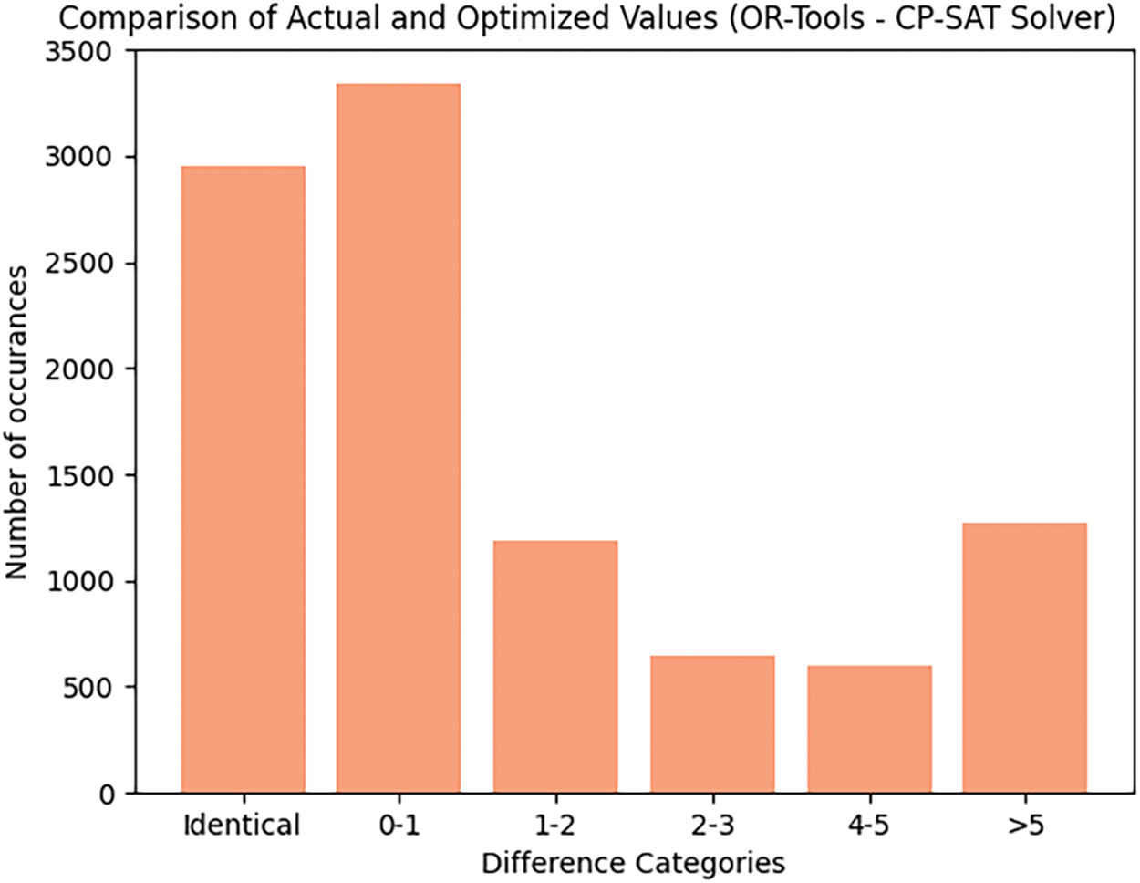
Figure 13: Results obtained by using the optimization method for one broadcaster

The second process begins with loading historical data on TV ad performances into a Dataframe object, which included various characteristics of the ads, such as their content categories, pricing information and previous scheduling times, as the target variable for prediction. From this dataset, we focus on the most impactful features that are expected to influence the success of the ads. This step is crucial for simplifying the analysis and focusing on factors that directly affect viewer engagement and ad performance.

To improve the effectiveness of the subsequent analysis, we integrate additional insights into the dataset. This included adding the optimized position from the previous step to suggest ideal ad placements. The aim is to create a more informed starting point for model training by incorporating these optimized ad positions as a new dimension in our dataset. The KNN model and its evaluation are guided by the objective to maintain a balance between achieving high viewer engagement and ensuring diversity in ad categories. The KNN model after post-processing achieves an exceptionally high level of accuracy with ~8400 exact matches. There are still some minor errors (~1600 occurrences), but no significant errors beyond a 1-category difference. The results after applying the post-processing function to the predicted positions are shown in Fig. 14.

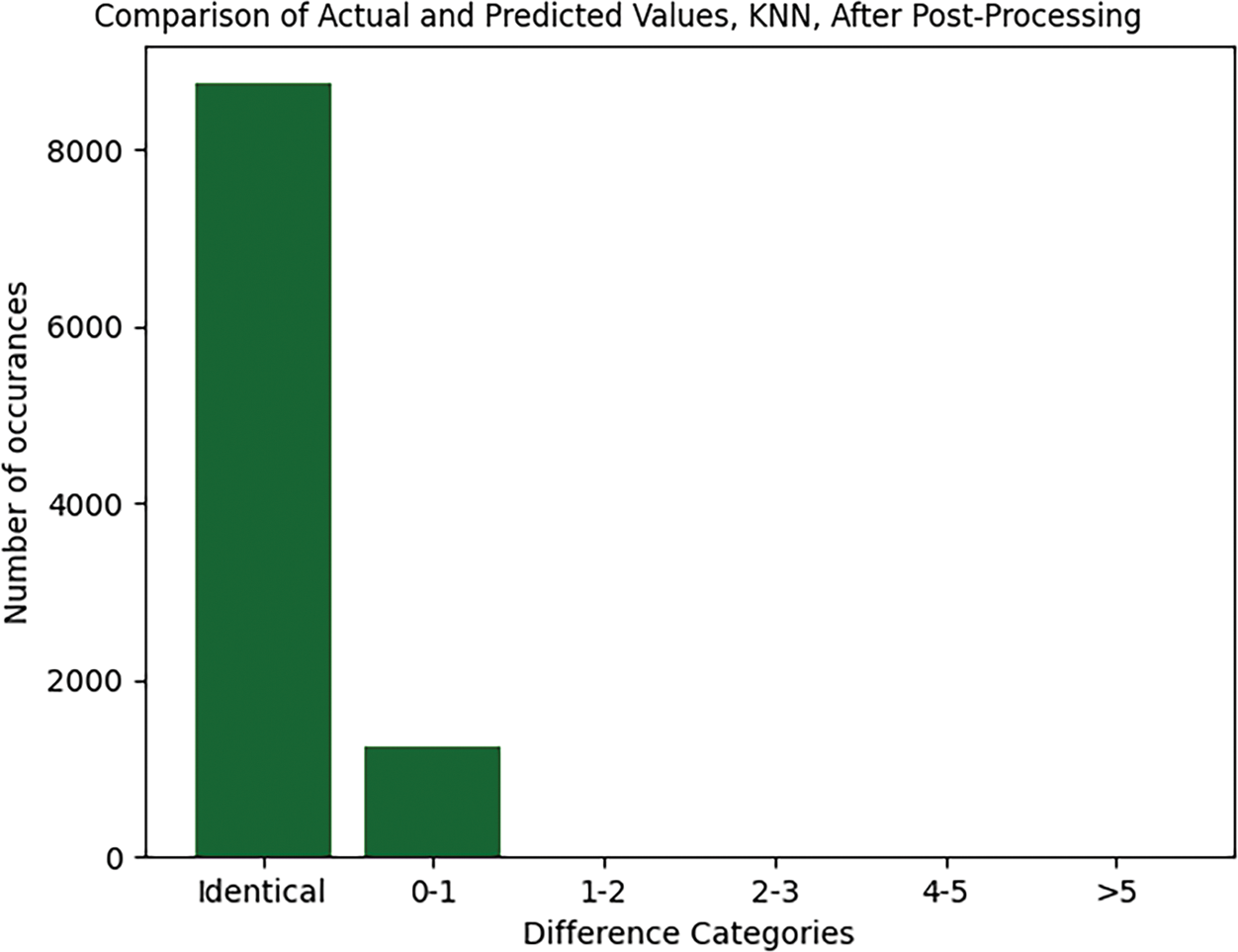
Figure 14: Results obtained after running KNN on the optimized positions

Before running the Federated Learning (FL) experiment, we use four datasets: for the first two positions are calculated using both category diversity constraint and the price constraint, and for the last ones we simulate data for user engagement rating and the price constraint. Initially, each client preprocesses its local dataset, focusing on relevant features that include ad category, price and user engagement metrics.

Each client trains a KNN model on its dataset, selecting a range of K values to evaluate. The models predict ad scheduling effectiveness based on features like ad category and price, aiming to optimize viewer engagement reflected in the user ratings. For each client, we define functions that calculate the meta-features. For the top n predictions made by the KNN model, we calculate price-related statistics (mean, median, standard deviation). Then, a simple count of unique categories within the top n predictions is applied to assess how well the model maintains ad content diversity. For the user engagement, we average user engagement, measured through ratings within the top n predicted ad placements. Each client evaluates its local KNN model by considering not just accuracy but also the calculated meta-features. Based on the aggregated insights from accuracy and meta-features evaluations, each client identifies the optimal K value for its KNN model. This value represents the best balance between accuracy, financial prudence, content diversity and expected viewer engagement. With the optimal K value identified, clients adjust their models accordingly and deploy them in their local environments. The results, after using the optimal K identified are shown in Fig. 15.

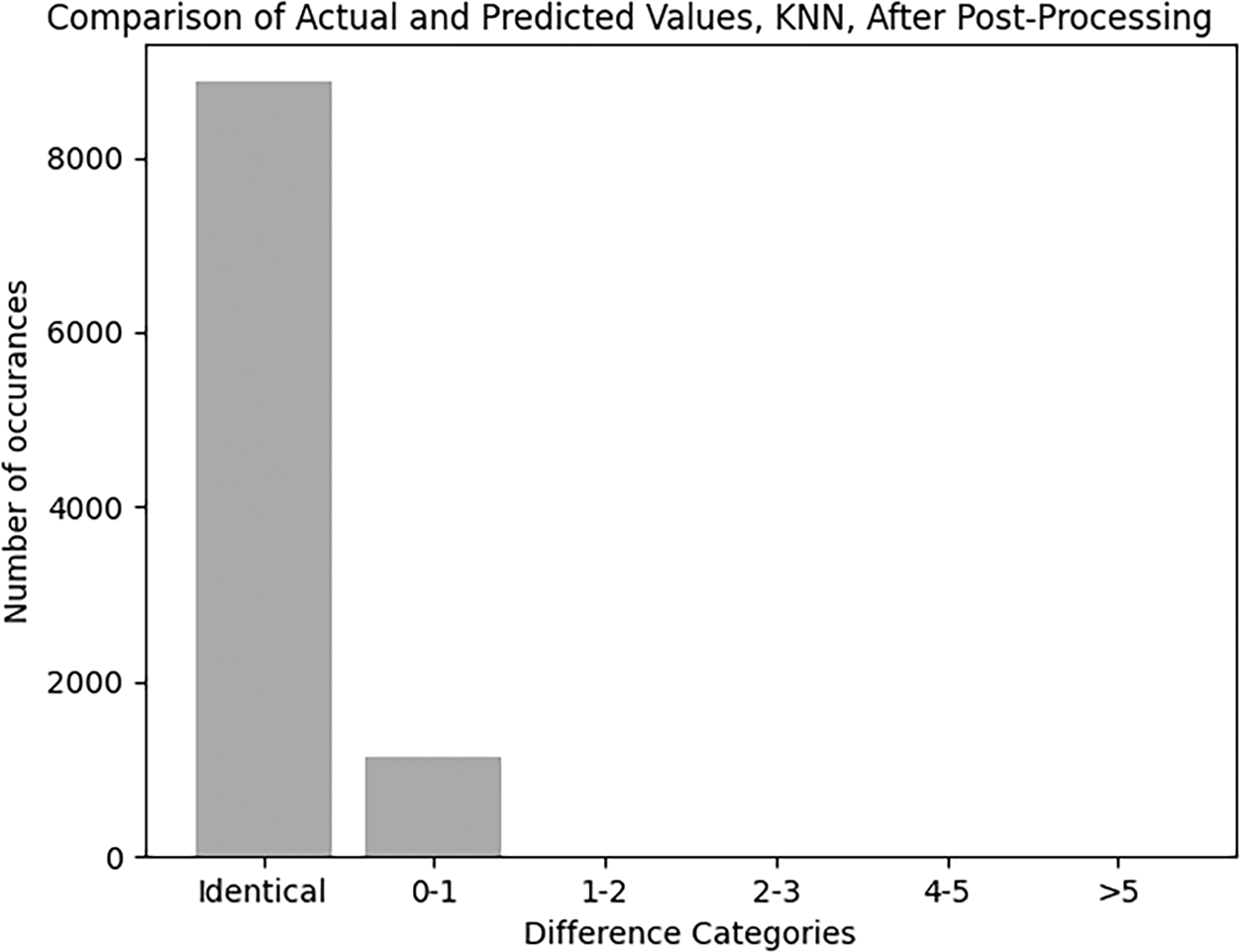
Figure 15: Results obtained after running the FL central server simulation

Continuous monitoring of model performance against real-world outcomes allows for dynamic adjustments, ensuring the ad scheduling strategy remains effective and responsive to changing viewer preferences and market conditions. In the FL setting, there were fewer than 200 additional correctly positioned ads compared to the results obtained without FL, indicating a slight improvement in accuracy. The results of the original KNN method showed that it could effectively predict ad placements, with a significant number of ads being placed close to their optimal positions. However, the FL-based KNN method introduced an additional layer of optimization by leveraging federated learning to aggregate insights from multiple broadcasters. This approach allowed the system to refine the predictions further, ensuring that the KNN models were better aligned with broader data trends and insights that individual broadcasters might not have access to.

Specifically, the FL-based KNN method resulted in 8650 ads being precisely matched to their optimal category placements, with a minimal deviation observed in 1350 ads, which were positioned within a one-category variance from their ideal placement. This slight improvement demonstrates how the FL approach enhances predictive accuracy and strategic insight across different networks compared to the original KNN method. In summary, while the original KNN method provided accurate predictions within individual datasets, the FL-based KNN method offered a more robust and refined solution by incorporating broader data insights, leading to better alignment with optimal ad placements across the network.

In the industry, KNN is less commonly used for ad spot prediction compared to more sophisticated models like Random Forest or Gradient Boosting because it can be computationally expensive and sensitive to the choice of K and feature scaling. However, in the model described, KNN performs well, particularly when combined with FL, which enhances its generalizability across multiple broadcasters’ data. However, post-processing is a common practice in the industry, especially in rule-based systems where final adjustments are made to ensure no violations of scheduling constraints. In this model, the post-processing step goes beyond traditional manual adjustments by programmatically enforcing diversity and placement rules.

This ensures that the predicted schedule aligns with both the pricing objectives (e.g., placing the highest-priced ads in prime positions) and category separation rules. The KNN model, when combined with post-processing, achieved a high level of accuracy, placing most ads in the optimal positions. The additional refinements during post-processing minimized errors and ensured compliance with business rules. With the inclusion of FL, the KNN model’s performance is enhanced across multiple broadcasters without the need to centralize sensitive data. This is a key advantage over traditional centralized ML models. Traditional models in the industry often rely on rule-based systems, where schedulers define static rules (e.g., highest-priced ads in key positions, no consecutive similar-category ads). These methods are simple but lack the flexibility and predictive power of ML-based models like KNN or Random Forest. The FL-based model learns from data rather than relying on static rules, allowing it to adapt to new patterns and trends, which is more effective than traditional rule-based systems.

The proposed model outperforms traditional methods by integrating ML to predict ad placements based on historical data and optimize them for key metrics like revenue, diversity and viewer engagement. By utilizing FL, the model trains across multiple broadcasters’ data without sharing sensitive information. Only model updates are exchanged, ensuring that data privacy is maintained.

Rule-based systems often require many iterations to enforce category diversity effectively, but this process can be time-consuming. The post-processing step in the model ensures that no consecutive ads belong to the same category, while still optimizing for high-value positions (first, second, last). This leads to a more engaging viewing experience and greater advertiser satisfaction. A brief comparison is provided in Table 3.

5  Discussions

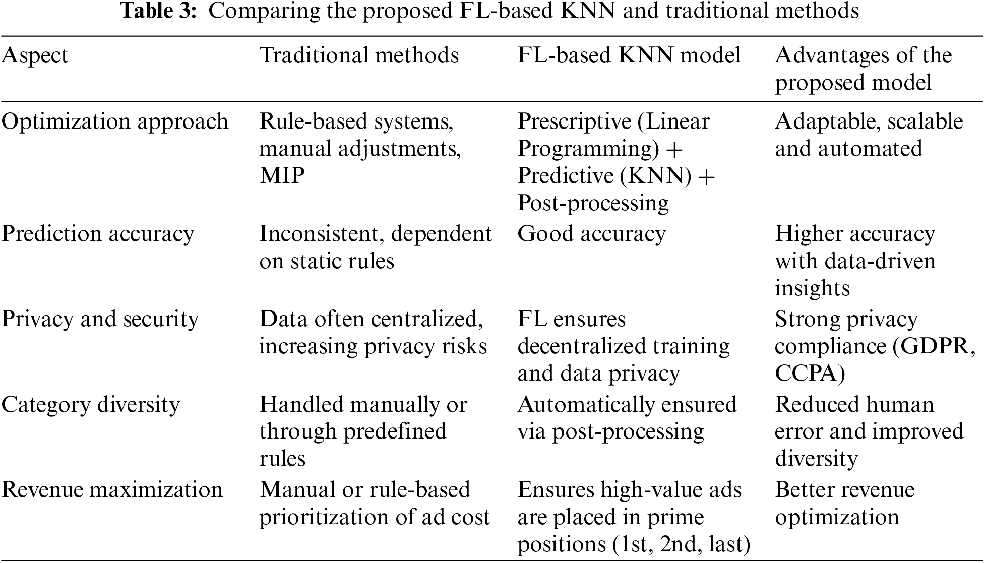
The process of aggregating model updates from an increasing number of clients becomes more complex as the system scales. Aggregating a large number of updates requires significant computational resources at the central server, and the complexity of this task grows with the number of participating clients. One potential approach to manage a growing number of clients could involve adopting a hierarchical FL structure. In this setup, clients can be grouped into clusters based on factors such as geographical or network proximity. Each cluster would perform a local aggregation of model updates before sending the results to the central server for final aggregation. This multi-level aggregation process helps reduce communication overhead and improves scalability by limiting the number of direct communications between individual clients and the central server. As the number of clients increases, the communication cost becomes a bottleneck. To address this, implementing advanced data compression techniques is considered to reduce the size of the model updates transmitted between clients and the server. Additionally, asynchronous communication protocols can be explored to allow clients to send their updates at different times, rather than synchronizing all clients. This approach ensures that the FL process continues smoothly without being delayed by slower clients, thus supporting a scalable system.

In a large-scale FL system, it may not be necessary for all clients to participate in every round of training. An adaptive participation mechanism can be developed, where a subset of clients is selected for each training round based on criteria such as data quality, client availability and computational capacity. Client sampling in FL is a technique where only a subset of clients participates in each training round. Random sampling is a specific method of client sampling where clients are randomly chosen to participate in each round of FL. This random selection helps ensure that the global model gradually incorporates insights from the entire population of clients without requiring every client to participate in every round. The random selection ensures that the global model integrates diverse data patterns, reducing the risk of overfitting to a specific client’s data. As a disadvantage, since not all clients participate in each round, the global model may converge more slowly compared to a scenario where all clients contribute to every round. The updates can be less representative in each round, requiring more rounds to achieve the same level of accuracy. The variance in updates is higher when only a subset of clients is used, potentially increasing the number of rounds needed for convergence. There is also a chance that some clients may be selected more frequently than others, especially in systems with a small number of rounds.

By utilizing FL, broadcasters optimize ad placements through the aggregation of diverse datasets, leading to more precise audience targeting. This precision enables broadcasters to command higher prices for ad slots, as the placements are more likely to reach the intended audience, thereby increasing the overall effectiveness of advertising campaigns. The shift from manual scheduling to an automated FL-based system usually leads to considerable cost reductions. The manual process is labor-intensive, requiring significant human resources to analyze data, predict viewer behavior and schedule ads accordingly. Automation through FL reduces these labor costs and also minimizes the likelihood of human error, which can lead to suboptimal ad placements and missed revenue opportunities. Additionally, the FL approach offers dynamic adaptability, allowing broadcasters to adjust ad schedules in near real-time based on aggregated insights from multiple sources. This capability to respond swiftly to changes in viewer behavior or market conditions provides a significant competitive edge, enabling broadcasters to maximize the use of available ad slots and improve their return on investment (ROI).

In traditional television networks, ad placement typically relies on a combination of manual processes and rule-based automated systems, both of which have been the industry standard for years. The process begins with audience segmentation, where broadcasters analyze demographics, viewing habits, and preferred time slots. This data is often gathered from established sources like Nielsen ratings and viewer surveys, along with other audience measurement tools. Through this segmentation, broadcasters determine which types of ads would be most effective during specific shows and time slots, allowing them to tailor their ad placements to the preferences and behaviors of their viewers. Ads are then placed based on the type of content being aired. For instance, a sports-related advertisement might be strategically scheduled during a live sports event, while ads for children’s toys might be placed during cartoons or family programming. This process often relies heavily on the manual decision-making of experienced schedulers who use their knowledge of audience preferences to optimize ad placements. These decisions are informed by historical data, which helps predict which time slots are likely to generate the most viewer engagement. The value of ad slots vary significantly depending on the time of day and the expected viewership. Prime-time slots, for example, are more expensive and are typically reserved for high-profile ads that are expected to reach a larger audience. In addition to manual scheduling, many networks use rule-based systems to assist in the process. These systems follow predefined rules established by human schedulers. For example, rules might be set to ensure that ads for competing products, such as well-known soft drinks, are not placed back-to-back, or that high-value ads are consistently placed at the beginning or end of commercial breaks where viewer attention is typically highest. While these rule-based systems automate certain aspects of ad scheduling, they are inherently limited by the quality and specificity of the rules programmed into them. They lack the flexibility and learning capability of more advanced systems, such as those driven by ML.

As airtime approaches, manual adjustments are often required to account for real-time factors such as live events running longer or shorter than expected, breaking news or sudden changes in audience size. This need for last-minute changes underscores the flexibility of manual scheduling and also introduces a higher risk of human error. Moreover, schedulers must ensure that ad placements comply with various regulatory requirements, particularly in programming aimed at children, where rules governing the timing and frequency of ads are especially stringent. These regulatory considerations add further complexity to the scheduling process. However, these traditional methods, while still widely used, have notable limitations. They are labor-intensive, reliant on static, historical data and prone to human error. They also lack the precision and adaptability needed to fully capitalize on real-time viewer behavior. In contrast, the proposed FL method offers a more advanced, data-driven approach.

6  Conclusions

Our research introduces a scalable, privacy-preserving ad scheduling system that improves predictive accuracy and strategic insights across multiple networks. The process begins with linear programming for initial schedule optimization, followed by a K-Nearest Neighbors (KNN) model to forecast ad placements. It employs a two-phase prescriptive-predictive framework: Google’s OR-Tools CP-SAT optimizes initial ad placements, forming a base schedule. This schedule then informs a predictive phase that strategically places additional ads based on ad attributes, enhancing scalability with models like KNN, LightGBM and Random Forest. Additionally, Federated Learning (FL) strengthens predictive performance and insights across networks, ensuring data confidentiality.

Utilizing Google’s OR-Tools CP-SAT solver, the model effectively maximized ad price visibility and ensured category diversity within ad breaks, with the dual objectives of augmenting viewer engagement and boosting advertising revenue. Initial optimization results revealed a substantial improvement in the strategic positioning of ads, aligning high-value ads at the beginning or end of breaks and maintaining category diversity to avoid repetition. This optimization was quantitatively assessed by comparing the original and optimized ad sequences: 4096 ads were within a one-slot deviation, 714 within a two-slot deviation, 602 within a three-slot deviation, 295 ads had a deviation between four and five slots, and 1044 ads deviated by more than five slots. Following the application of KNN predictions to the optimized ad scheduling, the evaluation metrics indicate a pronounced accuracy in maintaining category diversity, with 8865 ads being categorized identically to their optimal categorizations. Furthermore, a minor deviation was observed in 1248 ads with a one-category difference, and only 2 ads exhibited a two-category deviation. The Federated Learning (FL) method successfully aligned 8750 advertisements with their ideal category placements, reflecting the achievement of targeted diversity goals. Furthermore, a slight discrepancy was noted, with 1133 advertisements being placed just one category away from their perfect match in the initial dataset.

The proposed method reduces the post-processing effort and improves the results by generalization obtained by FL that includes other TV posts approaches. The fusion of ML models with federated optimization processes marks a significant advancement in ad scheduling strategies. This paper details how aggregated insights from across a network of broadcasters can be used to train global ML models. These models, in turn, predict the outcomes of various scheduling strategies, providing a richer understanding of viewer preferences and ad performance metrics. While promising, integrating FL with ML for ad scheduling optimization presents unique challenges, including data heterogeneity, the complexity of model aggregation and ensuring the relevance and quality of shared insights. Future implications of adopting a federated learning approach in TV ad scheduling to other domains is envisioned.

By harnessing the collective power of FL and ML, broadcasters improve the way TV ad schedules are optimized. This hybrid approach not only enhances the effectiveness of advertising campaigns, but also paves the way for a more collaborative, data-informed future in the broadcasting industry, all while maintaining strict adherence to privacy and data security standards.

Acknowledgement: This work was supported by a grant of the Ministry of Research, Innovation and Digitization, CNCS/CCCDI-UEFISCDI, project number COFUND-DUT-OPEN4CEC-1, within PNCDI IV.

Funding Statement: This work was supported by a grant of the Ministry of Research, Innovation and Digitization, CNCS/CCCDI-UEFISCDI, project number COFUND-DUT-OPEN4CEC-1, within PNCDI IV.

Author Contributions: Gabriela Dobrița: Investigation, Resources, Data Curation, Method, Writing—Original Draft, Validation, Formal Analysis; Simona-Vasilica Oprea: Validation, Formal Analysis, Investigation, Method, Writing—Original Draft, Writing—Review and Editing, Visualization, Project Administration; Adela Bâra: Conceptualization, Formal Analysis, Investigation, Resources, Data Curation, Writing—Original Draft, Writing—Review and Editing, Supervision. All authors reviewed the results and approved the final version of the manuscript.

Availability of Data and Materials: The data will be made available upon reasonable request.

Ethics Approval: Not applicable.

Conflicts of Interest: The authors declare no conflicts of interest to report regarding the present study.

References

1. A. Miklosík, P. Starchon, D. Vokounova, and M. Korcokova, “The future of TV advertising targeting young slovak consumers,” Mark. Manag. Innov., vol. 2, no. 2, pp. 122–138, 2020. doi: 10.21272/mmi.2020.2-09. [Google Scholar] [CrossRef]

2. I. A. Guitart, G. Hervet, and S. Gelper, “Competitive advertising strategies for programmatic television,” J. Acad. Mark. Sci., vol. 48, no. 4, pp. 753–775, 2020. doi: 10.1007/s11747-019-00691-5. [Google Scholar] [CrossRef]

3. R. Y. Du, L. Xu, and K. C. Wilbur, “Should TV advertisers maximize immediate online response?” SSRN Electron. J., 2017. doi: 10.2139/ssrn.3037734. [Google Scholar] [CrossRef]

4. Q. Yang, Y. Liu, T. Chen, and Y. Tong, “Federated machine learning: Concept and applications,” ACM Trans. Intell. Syst. Technol., vol. 10, no. 2, pp. 1–19, 2019. doi: 10.1145/3298981. [Google Scholar] [CrossRef]

5. C. Zhang, Y. Xie, H. Bai, B. Yu, W. Li and Y. Gao, “A survey on federated learning,” Knowl.-Based Syst., vol. 216, no. 1, 15 Mar. 2021, Art. no. 106775. doi: 10.1016/j.knosys.2021.106775. [Google Scholar] [CrossRef]

6. J. Wen, Z. Zhang, Y. Lan, Z. Cui, J. Cai and W. Zhang, “A survey on federated learning: Challenges and applications,” Int. J. Mach. Learn. Cybern., vol. 14, no. 2, pp. 513–535, 2023. doi: 10.1007/s13042-022-01647-y. [Google Scholar] [PubMed] [CrossRef]

7. J. Liu et al., “From distributed machine learning to federated learning: A survey,” Knowl. Inf. Syst., vol. 64, no. 4, pp. 885–917, 2022. doi: 10.1007/s10115-022-01664-x. [Google Scholar] [CrossRef]

8. A. Qammar, A. Karim, H. Ning, and J. Ding, “Securing federated learning with blockchain: A systematic literature review,” Artif. Intell. Rev., vol. 56, no. 5, pp. 3951–3985, 2023. doi: 10.1007/s10462-022-10271-9. [Google Scholar] [PubMed] [CrossRef]

9. B. Pfitzner, N. Steckhan, and B. Arnrich, “Federated learning in a medical context: A systematic literature review,” ACM Trans. Internet Technol., vol. 21, no. 1, pp. 1–31, 2021. doi: 10.1145/3412357. [Google Scholar] [CrossRef]

10. J. Xu, B. S. Glicksberg, C. Su, P. Walker, J. Bian and F. Wang, “Federated learning for healthcare informatics,” J. Healthc. Informatics Res., vol. 5, no. 1, pp. 1–19, 2021. doi: 10.1007/s41666-020-00082-4. [Google Scholar] [PubMed] [CrossRef]

11. K. Pillutla, S. M. Kakade, and Z. Harchaoui, “Robust aggregation for federated learning,” IEEE Trans. Signal Process., vol. 70, pp. 1142–1154, 2022. doi: 10.1109/TSP.2022.3153135. [Google Scholar] [CrossRef]

12. X. Li, S. Zhao, C. Chen, and Z. Zheng, “Heterogeneity-aware fair federated learning,” Inf. Sci., vol. 619, no. 5, pp. 968–986, Jan. 2023. doi: 10.1016/j.ins.2022.11.031. [Google Scholar] [CrossRef]

13. W. Zhou, “The choice of commercial breaks in television programs: The number, length and timing,” J. Ind. Econ., vol. 52, no. 3, pp. 315–326, 2004. doi: 10.1111/j.0022-1821.2004.00228.x. [Google Scholar] [CrossRef]

14. S. K. Reddy, J. E. Aronson, and A. Stam, “SPOT: Scheduling programs optimally for television,” Manage. Sci., vol. 44, no. 1, pp. 83–102, 1998. doi: 10.1287/mnsc.44.1.83. [Google Scholar] [CrossRef]

15. Y. -H. Li, L. Rasekh, and R. Jans, “Commercial advertisements scheduling problem,” DEStech Trans. Comput. Sci. Eng., 2020. doi: 10.12783/dtcse/cmso2019/33634. [Google Scholar] [CrossRef]

16. S. Seshadri, S. Subramanian, and S. Souyris, “Scheduling Spots on Television,” 2015. Accessed: Oct. 29, 2024. [Online]. Available: https://api.semanticscholar.org/CorpusID:55687110 [Google Scholar]

17. S. G. Domanal and G. R. M. Reddy, “An efficient cost optimized scheduling for spot instances in heterogeneous cloud environment,” Futur. Gener. Comput. Syst., vol. 84, no. 2, pp. 11–21, Jul. 2018. doi: 10.1016/j.future.2018.02.003. [Google Scholar] [CrossRef]

18. P. Rajaram, P. Manchanda, and E. M. Schwartz, “Finding the sweet spot: Ad scheduling on streaming media,” SSRN Electron. J., 2019. doi: 10.2139/ssrn.3496039. [Google Scholar] [CrossRef]

19. Y. Suzuki, W. M. Wee, and I. Nishioka, “TV advertisement scheduling by learning expert intentions,” in Proc. ACM SIGKDD Int. Conf. Know. Disc. Data Min., 2019, pp. 3071–3081. doi: 10.1145/3292500.3330768. [Google Scholar] [CrossRef]

20. F. Benali, D. Bodénès, C. De Runz, and N. Labroche, “A new reference-based algorithm based on non-euclidean geometry for multi-stakeholder media planning,” in Proc. ACM Symp. Appl. Comput., 2022, pp. 1056–1065. doi: 10.1145/3477314.3507320. [Google Scholar] [CrossRef]

21. V. M. Evangelista and R. G. Regis, “A multiobjective approach for maximizing the reach or GRP of different brands in TV advertising,” Int. Trans. Oper. Res., vol. 27, no. 3, pp. 1664–1698, 2020. doi: 10.1111/itor.12481. [Google Scholar] [CrossRef]

22. A. Goetzendorff, M. Bichler, R. Day, and P. Shabalin, “Core-pricing in large multi-object auctions: A market design for selling TV-ads,” SSRN Electron. J., 2013. doi: 10.2139/ssrn.2207140. [Google Scholar] [CrossRef]

23. A. Tanusondjaja, A. Michelon, N. Hartnett, and L. Stocchi, “Reaching voters on social media: Planning political advertising on snapchat,” Int. J. Mark. Res., vol. 65, no. 5, pp. 507–662, 2023. doi: 10.1177/14707853231175085. [Google Scholar] [CrossRef]

24. F. Benali, D. Bodenes, C. De Runz, and N. Labroche, “An enhanced R-NSGA-II for multiple brands advertising campaign allocation problem,” in 2021 IEEE 33rd Int. Conf. Tools Artif. Intell. (ICTAI), Washington, DC, USA, 2021. doi: 10.1109/ICTAI52525.2021.00206. [Google Scholar] [CrossRef]

25. A. Lambrecht, C. Tucker, and X. Zhang, “TV advertising and online sales: A case study of intertemporal substitution effects for an online travel platform,” J. Mark. Res., vol. 61, no. 2, pp. 185–392, 2023. doi: 10.1177/00222437231180171. [Google Scholar] [CrossRef]

26. J. Turner, “The planning of guaranteed targeted display advertising,” Oper. Res., vol. 60, no. 1, pp. 18–33, 2012. doi: 10.1287/opre.1110.0996. [Google Scholar] [CrossRef]

27. R. Y. Du, L. Xu, and K. C. Wilbur, “Immediate responses of online brand search and price search to TV ads,” J. Mark., vol. 83, no. 4, pp. 81–100, 2019. doi: 10.1177/0022242919847192. [Google Scholar] [CrossRef]

28. S. Purnamawati, E. B. Nababan, B. Tsani, R. Taqyuddin, and R. F. Rahmat, “Advertisement scheduling on commercial radio station using genetics algorithm,” J. Phy.: Conf. Ser., vol. 978, 2018, Art. no. 012113. doi: 10.1088/1742-6596/978/1/012113. [Google Scholar] [CrossRef]

29. M. Adler, P. B. Gibbons, and Y. Matias, “Scheduling space-sharing for internet advertising,” J. Sched., vol. 5, no. 2, pp. 103–119, 2002. doi: 10.1002/(ISSN)1099-1425. [Google Scholar] [CrossRef]

30. A. Freund and J. Naor, “Approximating the advertisement placement problem,” in Proc. 9th Int. IPCO Conf. Integer Programm. Combinat. Optimiz., 2004, pp. 415–424. doi: 10.1023/B:JOSH.0000036860.90818.5f. [Google Scholar] [CrossRef]

31. S. Kumar, M. Dawande, and V. S. Mookerjee, “Optimal scheduling and placement of internet banner advertisements,” IEEE Trans. Knowl. Data Eng., vol. 19, no. 11, pp. 1571–1584, 2007. doi: 10.1109/TKDE.2007.190640. [Google Scholar] [CrossRef]

32. G. Kim and I. Moon, “Online banner advertisement scheduling for advertising effectiveness,” Comput. Ind. Eng., vol. 140, no. 2, Feb. 2020, Art. no. 106226. doi: 10.1016/j.cie.2019.106226. [Google Scholar] [CrossRef]

33. L. L. C. Pedrosa, M. R. C. da Silva, and R. C. S. Schouery, “Approximation algorithms for the MAXSPACE advertisement problem,” Theory Comput. Syst., vol. 68, no. 3, pp. 571–590, 2024. doi: 10.1007/s00224-024-10170-2. [Google Scholar] [CrossRef]

34. D. G. Popescu and P. Crama, “Ad revenue optimization in live broadcasting,” Manage. Sci., vol. 62, no. 4, pp. 905–1224, 2016. doi: 10.1287/mnsc.2015.2185. [Google Scholar] [CrossRef]

35. H. Kim and K. S. Moon, “Optimal data construction in supervised machine learning for financial prediction,” Econ. Comput. Econ. Cybern. Stud. Res., vol. 58, no. 1, pp. 1–20, 2024. doi: 10.24818/18423264/58.1.24.01. [Google Scholar] [CrossRef]

36. G. Ke et al., “LightGBM: A highly efficient gradient boosting decision tree,” in 31st Conf. Neural Inf. Process. Syst. (NIPS 2017), Long Beach, CA, USA, 2017. [Google Scholar]

37. R. Genuer, J. M. Poggi, C. Tuleau-Malot, and N. Villa-Vialaneix, “Random forests for big data,” Big Data Res., vol. 9, no. 2, pp. 28–46, Sep. 2017. doi: 10.1016/j.bdr.2017.07.003. [Google Scholar] [CrossRef]