DecMamba: Mamba Utilizing Series Decomposition for Multivariate Time Series Forecasting

1  Introduction

Multivariate time series (MTS) forecasting is the task of predicting future information based on the historical information of multiple variables. MTS forecasting is widely used in the fields of finance [1,2], transportation [3,4], weather [5], and energy [6]. Recently, deep learning has achieved good prediction results in MTS forecasting tasks [7,8]. Cleveland et al. [9] denoted that separating long-term trends from cyclical variations is beneficial for analyzing complex time series. The various components after decomposition exhibit different underlying patterns. So, a better decomposition algorithm can help the model reveal the underlying patterns of the original series, thereby improving the accuracy of time series forecasting. Previous series decomposition algorithms [10–12] all use fixed kernels to decompose the original series into seasonal and trend components. However, for each variable of multivariate time series, the kernel of the series decomposition algorithm is fixed with the same value. Fixed kernels that only make fixed scale trends and periods interact with information make it difficult to analyze the complex trend correlations and periodic correlations between variables. This is detrimental to modeling the dependencies among different variables. The decomposed seasonal component exhibits stronger frequency fluctuations compared to the trend component. Previous decomposition-based forecasting models have overlooked the differences in sub-series frequency fluctuations between these two modes [10–12]. Transformer has become a mainstream model for MTS tasks, and previous Transformer-based [13] models [7,8,14–16] have achieved good results on MTS tasks. However, the disadvantage of its quadratic complexity in modeling the dependencies among different variables with variable dimensions that are too high leads to its high computation cost. To solve the above problems, we propose a Mamba model based on series decomposition, DecMamba. In DecMamba, we have designed a new decomposition module called Multivariate Adaptive Decomposition (MAD). MAD adopts a variable-level adaptive kernel search method to find the best set of kernel combinations that is most suitable for modeling the dependencies among different variables of seasonal and trend components in multivariate time series. DecMamba uses two different embedding methods to represent the trend and seasonal components separately. For the trend component, similar to iTransformer [17], we embed each variate of the trend component as a token and use Multilayer Perceptron (MLP) to model the temporal dependencies of the trend component easily. Considering its high-frequency fluctuations and semantically separable characteristics of the seasonal component, we have designed a new embedding block called Dimension Extension Embedding (DEE). DEE decomposes the seasonal component with a fixed time delay, and each seasonal sub-series is embedded into an independent token. Semantic information in seasonal components with high-frequency fluctuations is more easily obtained by univariate extending to multivariate. Furthermore, the fluctuation of the sub-series is smoother, and the semantic information is clearer than that of the original seasonal series. Due to the special embedding, the feature maps of seasonal components contain more complex information. Seasonal components using linear projection as a decoder [7,15] tend to make the decoder ignore important information. So, we introduce a gating mechanism to design a new Decoder, Gate Future Prediction (GFP). GFP uses an attention mechanism to score the final feature map of the seasonal component and scales it to the interval 0–1 as the weight matrix of representation. After the gating unit is completed, the important information in the feature map is compressed, and the noisy information is ignored. Finally, the prediction results of the seasonal component are obtained by a linear projection. Recently, the State Space Model (SSM), as a series modeling framework, has gradually become a popular tool in the field of time series analysis due to the virtue of its intrinsic mechanism of ordinary differential equations [18,19]. The ADSSM effectively translates PPG signals into ECG waveforms, showcasing the superior time series analysis capabilities of SSM [18]. Mamba [20], as an innovative extension of SSM, significantly improves the performance of traditional models by introducing a selection mechanism to filter useless information and dynamically adjust the state. Mamba also cleverly incorporates a hardware-aware design for efficient parallel training, making it a strong competitor to models like Transformer in tasks such as natural language understanding [21,22], audio waveform processing [23], computer vision [24–26], and point cloud learning [27]. Based on the linear complexity and high throughput of Mamba, we explore the application of Mamba in MTS by using it as a new master architecture to model the dependencies among different variables. In summary, our contributions are as follows:

1.    We design a new decomposition algorithm, Multivariate Adaptive Decomposition (MAD), which can dynamically decompose each variable series in a multivariate time series. The optimal combination of kernels for decomposition is searched for multivariate time series at the variable level to facilitate better modeling the temporal dependencies and the dependencies among different variables.

2.    Aiming at the characteristics of high-frequency fluctuation of seasonal components after series decomposition, a new Embedding module, Dimension Extension Embedding (DEE), is designed, which can decompose a single seasonal variable into multiple sub-seasonal variables. DEE can reduce the high-frequency fluctuation of the seasonal series, simplify the semantic information of the seasonal component, and capture the temporal dependency of the seasonal component in a better way with dimension expansion.

3.    A new prediction module, Gate Future Prediction (GFP), is designed for seasonal components after series decomposition. This module enables the prediction layer to focus on the important information of seasonal series and ignore the noise information.

4.    The linear complexity and high throughput of Mamba make it an alternative to replace the Transformer. Based on the superior performance of Mamba in other domains, we use it as a new master architecture for the dependencies among different variables modeling to explore the application of Mamba in the MTS domain.

5.    Based on the above improvements, a new architecture, DecMamba, for multivariate time series forecasting is proposed. Its better forecasting performance is verified by comparing it with ten SOTA models on seven real-world datasets.

2  Related Works

2.1 Multivariate Time Series Forecasting

MTS prediction models can be broadly classified into statistical models and deep learning models. The traditional statistical models are no longer sufficient to meet the current prediction needs of MTS. Due to the superior fitting capabilities, deep learning models are now commonly used as the main architecture for MTS. When modeling dependencies among different variables in multivariate series, deep models typically incorporate three approaches: local channel mixing, global channel mixing, and independent channels. Local channel mixing generally considers multidimensional information at a single time step independently and then captures the temporal dependencies of the series. For example, Recurrent Neural Networks (RNNs) are commonly used for multivariate time series (MTS) tasks. LSTM [28] and GRU [29] introduce gating mechanisms to mitigate the vanishing gradient issue in long sequences. LSTNet [30] improves multivariate time series forecasting by capturing both short-term and long-term patterns. DeepAR [31] enhances the robustness of the model by generating probabilistic forecasts through Monte Carlo sampling. Wen et al. [32] proposed a BiLSTM with temporal pattern attention for ignoring irrelevant information and amplifying the required information. TCN [33] in CNN introduces causal convolution to simulate the temporal relationships in the series with the method of local channel mixing. SCINet [34] in CNN repeatedly extracts and exchanges information at different time resolutions and learns effective representations to improve predictability. SCINet has shown significant advantages in traffic flow forecasting tasks [35]. Transformer models such as Informer [16], Autoformer [10], FEDformer [12], and Stationary [14] use point tokens to mix channels locally. Autoformer, FEDformer, and Stationary have achieved good results in Traffic, Weather, and finance tasks, respectively [36–38]. Crossformer [8] proposes a two-stage Routing Attention mechanism that extracts all dependencies among different variables by routing tokens to each variable. This approach also extends the scope of individual token information due to the patch embedding method. Crossformer has been applied in practical power load forecasting tasks [39]. However, the method of local channel mixing has limitations due to the different sampling frequencies of multiple variables and the semantic gap between them. PatchTST [15] model adopts an independent channel modeling approach, which enhances the robustness of the model by avoiding channel mixing. PatchTST has accurately predicted the air quality index [40]. TimesNet [17] in the CNN model and Dlinear [11] in the MLP model also use the independent channel approach for MTS prediction. TimesNet and Dlinear are widely used in finance and energy domains, respectively [41,42]. TIDE [43] completes the encoding and decoding work based on MLP. However, focusing solely on modeling temporal dependencies while neglecting the dependencies among different variables does not optimally analyze multivariate time series. iTransformer [7] treats individual variate as independent tokens and uses self-attention to model dependencies among different variables. iTransformer is a global channel-mixing approach.

2.2 Time Series Decomposition

Autoformer [10], PEDformer [12], and Dlinear [11], all separate long-term trends from cyclical variations to achieve series decomposition. Autoformer and PEDformer utilize the decomposition block as an internal operator and replace the self-attention mechanism with auto-correlation to model the temporal dependencies in the series. Dlinear first decomposes the original series into trend and seasonal components. Linear networks are used to predict the future information of each component, and the prediction results are summed up to obtain the final forecasting result. However, the aforementioned approaches neglect the different frequencies between the trend component and seasonal component. They also disregard the potential impact that different combinations of trend components and seasonal components among variables could have on forecast accuracy.

3  Methods

In MTS forecasting, our goal is to predict future values XT based on multivariate historical data input X. Let X∈RL×C represent an MTS with C variables and a history window L of length. Similarly, let XT∈RL×C represent a multivariate time series with C variables and a forecasting window T of length. To achieve higher prediction accuracy, we propose a model called DecMamba.

3.1 Model Structure

The overall architecture of DecMamba is shown in Fig. 1. DecMamba uses Multivariate Adaptive Decomposition (MAD) to perform adaptive decomposition operations on MTS. This process produces trend component Xtrend∈RL×C, which represents the inconsistent trend changes among different variables, and seasonal component Xseasonal∈RL×C, which captures the inconsistent periodic changes among variables. Aligned to the right margin:

Figure 1: Overall architecture of DecMamba, which consists of Multivariate Adaptive Decomposition, Seasonal Backbone, and Trend Backbone for series decomposition, respectively

Xtrend,Xseasonal=MAD(X)(1)

Due to the differences in frequency fluctuations between the trend component and seasonal component, two distinct network structures were designed. The Seasonal Backbone (SB) is responsible for forecasting the future values of the seasonal component, while the Trend Backbone (TB) is dedicated to forecasting the future values of the trend component. The two distinct network structures allow DecMamba to effectively predict the two underlying patterns separately.

X^trend=TB(Xtrend)(2)

X^seasonal=SB(Xseasonal)(3)

The final forecasting result output Y is obtained by summing.

Y=X^seasonal+X^trend(4)

3.2 Multivariate Adaptive Decomposition

Previous series decomposition algorithms have often used series decomposition with a fixed kernel. The process is as follows:

Xtrend=AvgPool(Padding(X)kernel(5)

Xseasonal=X−Xtrend(6)

Unlike traditional fixed kernel decomposition algorithms [10–12], MAD finds the optimal combination of decomposition kernels for MTS during the training process with an adaptive search method. The method is as follows:

3.2.1 Initialization

m kernels kernelall with varying sizes, Cost matrix CM and Count Matrix Count are initialized. kernelall is used to represent the search space of kernels. CM records the cost during the training process. Count records the frequency of each kernel selected by the variables during the training process.

3.2.2 Training

w∗C kernels are randomly selected in kernelall and divided into w group kernel combinations. Each kernel combination contains C kernels, where w<<batchsize. The same kernel can be repeatedly selected. Input X of the original batch is divided into w mini-batches that are decomposed by the w kernel combinations. The process is as follows:

Xtrendi,j=AvgPool(Padding(Xi,j)kernelrandi(7)

Xseasonali,j=Xi,j−Xtrendi,j(8)

lcj=1bsw∑p=1bsw|Yp,j−XTp,j|(9)

CMki=CMki+(lcj−1w∑q=1wlcq)(10)

CMki represents the cost of the overall prediction outcome when the ith variable chooses the kth kernel as part of the decomposition combination.

3.2.3 Inference

The optimal combination of kernel kernelbest is selected from kernelall according to CM. Because CMki represents the cost of the prediction outcome for all variables rather than for individual variables. The ith variable uses kmeanth kernel to decompose, which can minimize the overall prediction outcome cost.

CMkmeaniCountkmeani=min(CM1iCount1i,…,CMkiCountki,…,CMwiCountwi)(11)

Countki denotes the number of times the kth kernel is chosen by the ith variable. The original series will be decomposed by kernelbest to obtain the combinations of trend and seasonal components that are most conducive to modeling the dependencies among different variables. During inference, the process is as follows:

Xtrend=AvgPool(Padding(X)kernelbest(12)

Xseasonal=X−Xtrend(13)

3.3 Trend Backbone

Trend Backbone (TB) is composed of Embedding, Encoder (TE), and Future Prediction (FP). TB uses the instance normalization operations and embedding block as same as iTransformer [7]. TB embeds each time series of Xtrend as variate tokens htrend. For TE, given the embedded trend component hidden variables htrend, the output is a feature map h^trend of the trend component.

h^trend=TE(htrend)(14)

TE uses Mamba to model the dependencies among different variables. The internal structure of Mamba is shown in Fig. 2, where the left branch is a gated nonlinear layer, and the right branch serves as a linear time-invariant (LTI) system (SSM). The temporal dependencies are modeled using a feedforward network (FFN). For the lth layer, the input is htrendl−1, and the output is htrendl. The process of TE can be formalized as:

Figure 2: Mamba block

htrendl=FFN(SSM(Conv(Linear(htrendl−1)))+σ(Linear(htrendl−1)))(15)

htrend is the input of layer 1, and h^trend is the output of the last layer. FP directly outputs the prediction results of the trend component through a simple linear projection.

X^trend=FP(h^trend)(16)

3.4 Seasonal Backbone

The Seasonal Backbone (SB) consists of the Dimension Extension Embedding (DEE), an Encoder (SE), and the Gate Future Prediction (GFP) module.

3.4.1 Dimension Extension Embedding

DEE embeds the seasonal component by expanding its dimensions. To more effectively embed the future map of the decomposed seasonal component, DEE achieves semantic segmentation of seasonal components through dimension expansion. Given the inputs XseasonalϵRL×C, the sampled components are obtained based on sub-sampling according to a fixed time delay. XseasonalϵRL×C is expanded into an extended time series XsampleϵRLs×delay×C of length Ls and dimension delay×C. This extended series XsampleϵRLs×delay×C is then embedded as separate tokens hseasonal to represent the hidden variables of the seasonal component. Compared to trend embedding methods [7], DEE is better suited for embedding high-frequency series like seasonal series, making the semantic information represented by the embedded tokens clearer.

3.4.2 Seasonal Encoder

The encoder of the seasonal component SE is the same as TE.

h^seasonal=SE(hseasonal)(17)

For the lth layer, the input is hseasonall−1, and the output is hseasonall. The process of SE can be formalized as follows:

hseasonall=FFN(SSM(Conv(Linear(hseasonall−1)))+σ(Linear(hseasonall−1)))(18)

hseasonal is the input of layer 1, and h^seasonal is the output of the last layer. SB then outputs the prediction results of the seasonal component through GFP, which acts as a decoder.

X^seasonal=GFP(h^seasonal)(19)

where X^seasonalϵRT×C represents the prediction results of the Seasonal Backbone.

3.4.3 Gate Future Prediction

GFP introduces a gating mechanism to enhance the accuracy of the prediction results. This is done by taking the embedded seasonal component representation, performing a matrix projection through a linear layer to obtain the importance score matrix, and normalizing the score to a range between 0 and 1 using a sigmoid activation function. The score matrix is then multiplied with the seasonal component representation to obtain a more accurate representation. The final prediction of the seasonal component is obtained through a linear projection, similar to the FP process in the Trend Backbone.

X^seasonal=Linear(sigmoid(Linear(h^seasonal))∗h^seasonal)(20)

4  Experiments

4.1 Dataset

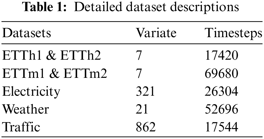
We conducted extensive experiments on seven real-world datasets [10], as shown in Table 1, including ETT datasets (including four subsets: ETTh1, ETTh2, ETTm1, ETTm2), Weather, Electricity, Traffic, and Exchange covering domains such as electricity, energy, transportation, weather, and finance.

4.2 Baselines and Metrics

To demonstrate the effectiveness of DecMamba on the MTS task, ten popular SOTA models were selected for comparison. The baseline models include Autoformer [10], FEDformer [12], Stationary [14], Crossformer [8], PatchTST [15], DLinear [11], TiDE [43], SCINet [34], TimesNet [17], iTransformer [7]. Crossformer and DLinear are SOTA models in the domain of energy [39,42]. Autoformer and SCINet are SOTA models in the domain of transportation [35,36]. FEDformer and PatchTST are SOTA models in the domain of weather [37,40]. Stationary and TimesNet are SOTA models in the domain of finance [38,41]. To measure the prediction performance of multiple models on multiple datasets, Mean Squared Error (MSE) and Mean Absolute Error (MAE) are used as evaluation metrics.

4.3 Implementation Details

Experiments were performed using the Adam optimizer [44] on two NVIDIA T4 16 GB GPUs. The training was performed 10 times with early stopping using patience 3 to avoid overfitting.

4.4 Main Results

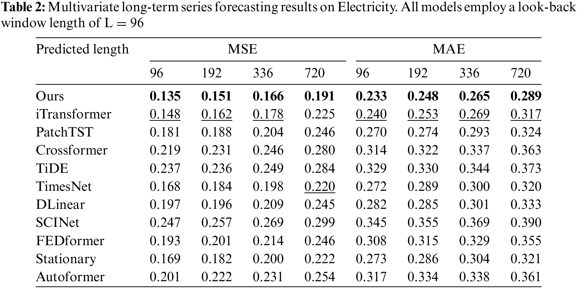
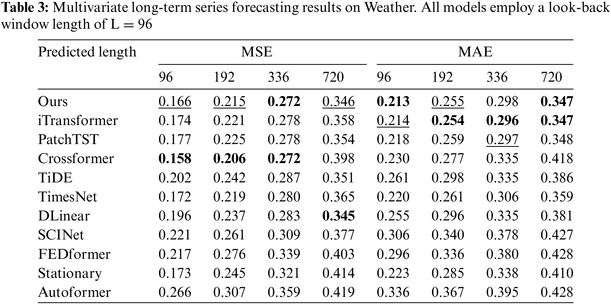
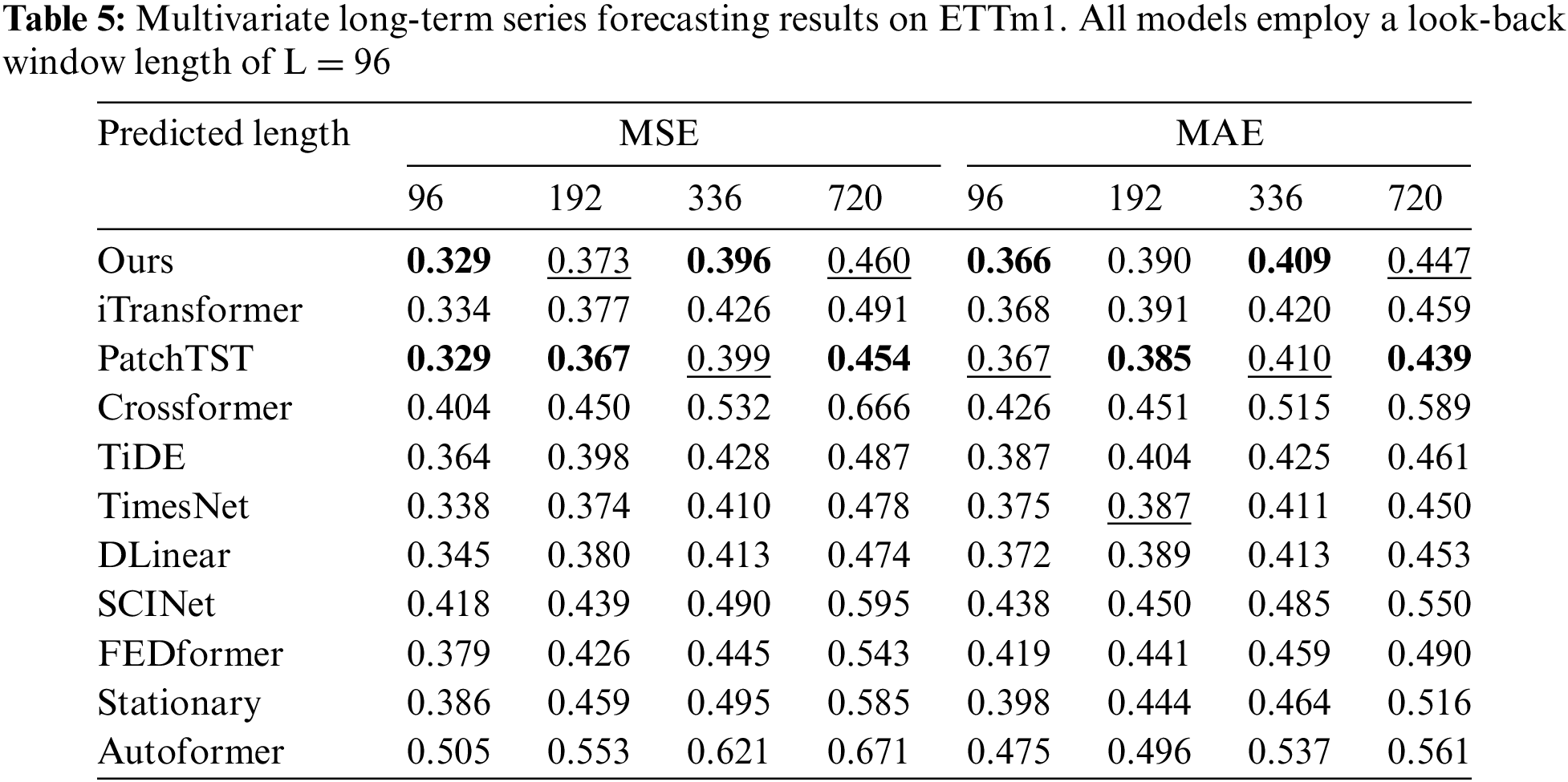
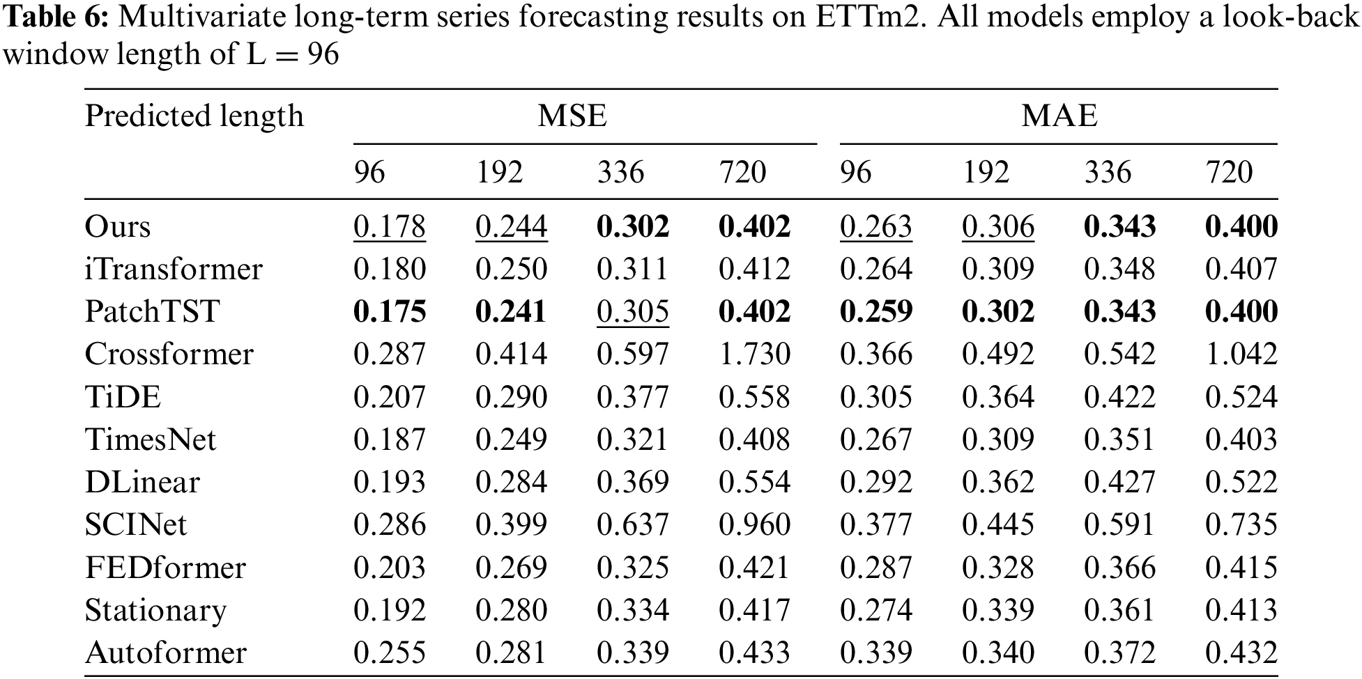
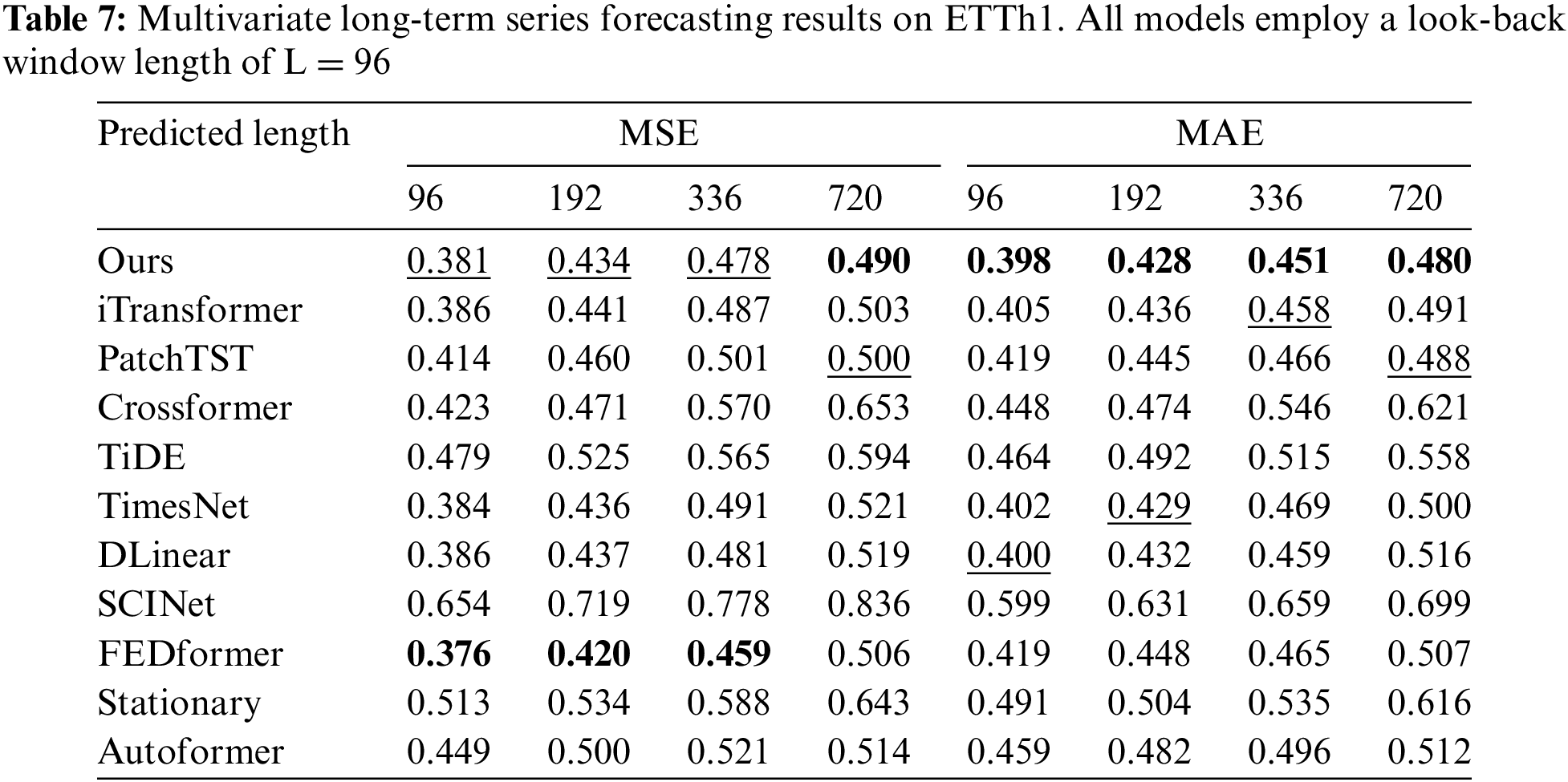
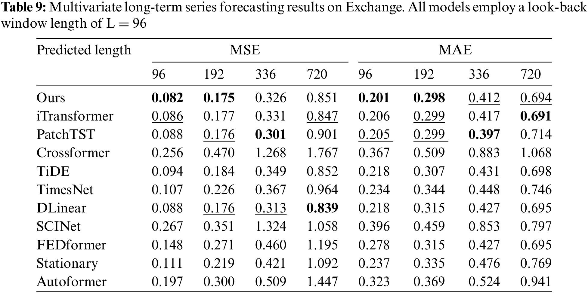
Comprehensive forecasting results are listed in Tables 2–9, with the best in bold and the second underlined. The lower MSE/MAE indicates the more accurate prediction result. Overall, DecMamba shows leading performance on most datasets, as well as on different prediction length settings, with 34 top-1 and 52 top-2 cases out of 56 in total. DecMamba performs even better on datasets with a large number of variables like Weather, Electricity, and Traffic. In particular, DecMamba produces all SOTA results on Electricity in MTS forecasting. The variable number of Exchange datasets in finance is less and the time series of financial domains usually include irregular seasonal components [38]. Under such extreme conditions, our model still achieves the 4 top-1 and 6 top-2 ranks across 8 evaluation metrics. The results on the Exchange dataset validate the model’s ability to generalize for different types of time series. Compared to SOTA models in various domains, our model has performed well. In the Electricity dataset, our model outperforms Crossformer and DLinear on all metrics. In the Weather dataset, our model surpasses PatchTST on 87.5% of metrics. In the Traffic dataset, our model exceeds Autoformer and SCINet in all metrics, while in the Exchange dataset, it outperforms Stationary and TimesNet in all metrics. iTransformer is the previous best model on MTS forecasting. Our model outperforms iTransformer on 83.93% of the evaluation metrics with all prediction lengths in all datasets.

4.5 Model Efficiency

We analyze the computational complexity of our models and baseline models. In Table 10, C represents the number of variables, L is the sequence length, P refers to the patch size, and Lseg denotes the segment length in Crossformer. Models like Autoformer, Stationary, FEDformer, and SCINet, which embed variables into tokens at each time step, have complexity dependent only on L. However, excessively local receptive fields may reduce prediction accuracy. Channel-independent models like TiDE, DLinear, TimesNet, and PatchTST scale linearly with C. Crossformer also shows linear complexity in C, while iTransformer is quadratic. Due to the linear complexity of Mamba, the token of DecMamba aggregates the global representations but is only linearly with L.

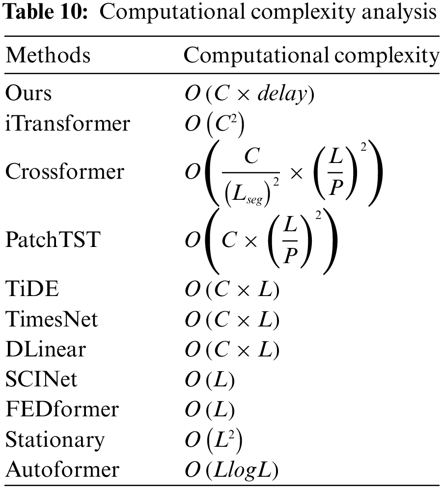
FEDformer, PatchTST, and iTransformer in Transformer are representative models of three modeling methods, respectively. We compare the running time and memory consumption of our model with these models on traffic and ETTh2 datasets. As shown in Fig. 3, on the ETTh2 dataset with fewer variables, FEDformer has the highest memory and training time. Our model’s memory usage is similar to iTransformer and PatchTST, with a slightly longer training time. However, on the Traffic dataset (with more variables), iTransformer and PatchTST show significant increments in memory and time, while the complexity increment of our model is not evident compared to these models. These results show that Mamba is more efficient compared to Transformer, and our model has better scalability and applicability in real-world applications.

Figure 3: Comparison of our model and three baselines on Training Time, and GPU Memory. All versions employ a look-back window length of L = 96 and a predicted length of T = 96 on Traffic and Etth2 datasets

4.6 Visualize the Optimal Combination of Kernels

As shown in Fig. 4, the sizes of optimal decomposition kernel combinations are obtained by MAD on ETTh1 and Exchange datasets. The sizes on ETTh1 are different from Exchange. MAD tends to select larger sizes of decomposition kernel combinations to decompose original series on Exchange. Compared with ETTh1, Exchange exhibits more complex or irregular seasonality. The decomposition kernel combinations with larger sizes can make trend components with clearer trend information and seasonal components with more original information. So better prediction performance can be obtained. The kernel sizes assigned to each variable in ETTh1 and Exchange datasets differ. These kernel sizes are adjusted with the prediction results during the training process. MAD adaptively selects suitable decomposition kernel combinations according to the characteristics of datasets. Accurate prediction results can be obtained by optimizing decomposition with a better generalization ability for various types of multivariate time series.

Figure 4: Visualization of the optimal combination of kernels

4.7 Impact of the Number of Variables on Model Performance

In this section, we analyze how the number of variables affects the performance of our model. We conducted a controlled experiment using the Electricity dataset. The number of input variables is set to 20%, 60%, and 100% of the original variables. The number of output variables is uniformly set to 20% of the original variables. Table 11 shows that increasing the number of input variables improves prediction accuracy. Memory consumption increases with the increment of input variables, but training time remains stable. These results indicate that our model effectively captures the dependencies among additional and output variables. Our model demonstrates scalability and robustness in scenarios with varying numbers of variables.

4.8 Ablation Studies and Analyses

4.8.1 Component Ablation

We removed the corresponding modules to perform ablation studies on the Electricity. W/O-MAD uses a traditional decomposition that is a fixed decomposition kernel instead of MAD. The embedding method of W/O-DEE is similar to itransformer [7] instead of DEE. W/O-GFP replaces GFP in the original decoder [7,15]. As shown in Table 12, the prediction performance of W/O-MAD and W/O-DEE is significantly lower than our original model. Especially in the long series tasks, performance degradation is very obvious. This experiment can demonstrate that MAD can decompose original series into the trend and seasonal component combinations, which are more suitable for modeling the dependencies among different variables. DEE is more conducive to the representation and prediction of seasonal components. GFP is more robust than the original decoder [7,15], resulting from focusing on the valid information of the high-frequency seasonal components by ignoring noise information.

4.8.2 Study on Hyperparameter Sensitivity

delay is an important parameter of DEE, and the length of delay directly affects the complexity of semantic information in a single seasonal component. We set the length of delay to 4, 6, and 8, respectively, to evaluate the performance of our models on Electricity. As shown in Table 13, with delay length 6, the best performance can be obtained.

5  Conclusion

We propose a model called DecMamba for multivariate time series (MTS) forecasting. DecMamba addresses the limitations of previous series decomposition algorithms with MAD searching for kernels adaptively. DEE, a new embedding method, overcomes the shortcomings of previous methods struggling to capture the semantic information in high-frequency seasonal components. A decoder called GFP with a gating mechanism is designed to minimize the impact of unnecessary information from the seasonal component. The experiment results show that MAD better resolves complex trend and period dependencies among variables, DEE enhances the ability to extract semantic information in seasonal components by improving prediction performance, and GFP improves robustness. Additionally, the main architectural structure with Mamba throughput is increased, and the complexity of excessive time is reduced. DecMamba excels in capturing the dependencies among different variables compared to seven real-world datasets. Varying in prediction lengths and metrics, DecMamba ranks first among the ten models in 34 out of 56 settings and achieves the top 2 in 52 of them.

Acknowledgement: We thank the members of the Communication and Network Key Laboratory for their contributions to this work.

Funding Statement: This work was supported in part by the Interdisciplinary Project of Dalian University (DLUXK-2023-ZD-001).

Author Contributions: The authors confirm contribution to the paper as follows: study conception and design: Jianxin Feng and Jianhao Zhang; data collection: Jianhao Zhang; analysis and interpretation of results: Jianxin Feng and Jianhao Zhang; draft manuscript preparation: Jianxin Feng, Jianhao Zhang, Ge Cao, Zhiguo Liu and Yuanming Ding. All authors reviewed the results and approved the final version of the manuscript.

Availability of Data and Materials: All datasets are collected by Reference [10], and they are openly available at https://github.com/thuml/Autoformer (accessed on 10 September 2024).

Ethics Approval: Not applicable.

Conflicts of Interest: The authors declare no conflicts of interest to report regarding the present study.

References

1. W. Yin, Z. L. Chen, X. X. Luo, and B. Kirkulak-Uludag, “Forecasting cryptocurrencies’ price with the financial stress index: A graph neural network prediction strategy,” Appl. Econ. Lett., vol. 31, no. 7, pp. 630–639, 2024. doi: 10.1080/13504851.2022.2141436. [Google Scholar] [CrossRef]

2. J. Wang and J. Wang, “A new hybrid forecasting model based on SW-LSTM and wavelet packet decomposition: A case study of oil futures prices,” Comput. Intell. Neurosci., vol. 2021, no. 1, 2021, Art. no. 7653091. doi: 10.1155/2021/7653091. [Google Scholar] [PubMed] [CrossRef]

3. Q. Y. Luo, S. L. He, X. Han, Y. H. Wang, and H. F. Li, “LSTTN: A long-short term transformer-based spatiotemporal neural network for traffic flow forecasting,” Knowl.-Based Syst., vol. 293, no. 2, 2024, Art. no. 111637. doi: 10.1016/j.knosys.2024.111637. [Google Scholar] [CrossRef]

4. J. H. Chen, L. Yang, C. Qin, Y. Yang, L. Peng and X. T. Ge, “Heterogeneous graph traffic prediction considering spatial information around roads,” Int. J. Appl. Earth Obs. Geoinf., vol. 128, 2024, Art. no. 103709. doi: 10.1016/j.jag.2024.103709. [Google Scholar] [CrossRef]

5. H. Balti, A. B. Abbes, and I. R. Farah, “A Bi-GRU-based encoder-decoder framework for multivariate time series forecasting,” Soft Comput., vol. 28, no. 9–10, pp. 6775–6786, 2024. doi: 10.1007/s00500-023-09531-9. [Google Scholar] [CrossRef]

6. S. Smyl, G. Dudek, and P. Pelka, “Contextually enhanced ES-dRNN with dynamic attention for short-term load forecasting,” Neural Netw., vol. 169, no. 2, pp. 660–672, 2024. doi: 10.1016/j.neunet.2023.11.017. [Google Scholar] [PubMed] [CrossRef]

7. Y. Liu et al., “iTransformer: Inverted transformers are effective for time series forecasting,” in Twelfth Int. Conf. Learn. Represent., Kigali, Rwanda, 2024. [Google Scholar]

8. Y. H. Zhang and J. C. Yan, “Crossformer: Transformer utilizing cross-dimension dependency for multivariate time series forecasting,” in Eleventh Int. Conf. Learn. Represent., Kigali, Rwanda, 2023. [Google Scholar]

9. R. B. Cleveland, W. S. Cleveland, J. E. McRae, and I. Terpenning, “STL: A seasonal-trend decomposition procedure based on loess,” J. Off. Stat., vol. 6, no. 3, pp. 3–73, 1990. [Google Scholar]

10. H. X. Wu, J. H. Xu, J. M. Wang, and M. S. Long, “Autoformer: Decomposition transformers with auto-correlation for long-term series forecasting,” in Adv. Neural Inf. Process. Syst., Montreal, QC, Canada, 2021, vol. 34, pp. 22419–22430. [Google Scholar]

11. A. L. Zeng, M. X. Chen, L. Zhang, and Q. Xu, “Are transformers effective for time series forecasting?,” Proc. AAAI Conf. Artif. Intell., vol. 37, no. 9, pp. 11121–11128, 2023. doi: 10.1609/aaai.v37i9.26317. [Google Scholar] [CrossRef]

12. T. Zhou, Z. Q. Ma, Q. S. Wen, X. Wang, L. Sun and R. Jin, “FEDformer: Frequency enhanced decomposed transformer for long-term series forecasting,” in Proc. 39th Int. Conf. Mach. Learn., Baltimore, MD, USA, 2022, vol. 162, pp. 27268–27286. [Google Scholar]

13. Vaswani et al., “Attention is all you need,” in Adv. Neural Inf. Process. Syst., Long Beach, CA, USA, 2017, vol. 30. [Google Scholar]

14. Y. Liu, H. X. Wu, J. M. Wang, and M. S. Long, “Non-stationary transformers: Exploring the stationarity in time series forecasting,” in Adv. Neural Inf. Process. Syst., Long Beach, CA, USA, 2022, vol. 35, pp. 9881–9893. [Google Scholar]

15. Y. Nie, N. H. Nguyen, P. Sinthong, and J. Kalagnanam, “A time series is worth 64 words: Long-term forecasting with transformers,” in Eleventh Int. Conf. Learn. Represent., Kigali, Rwanda, 2023. [Google Scholar]

16. H. Y. Zhou et al., “Informer: Beyond efficient transformer for long sequence time-series forecasting,” Proceedings AAAI Conf. Artifi. Intell., vol. 35, no. 12, pp. 11106–11115, 2021. doi: 10.1609/aaai.v35i12.17325. [Google Scholar] [CrossRef]

17. H. X. Wu, T. G. Hu, Y. Liu, H. Zhou, J. M. Wang and M. S. Long, “TimesNet: Temporal 2D-variation modeling for general time series analysis,” in Eleventh Int. Conf. Learn. Represent., Kigali, Rwanda, 2023. [Google Scholar]

18. K. Vo, M. El-Khamy, and Y. Choi, “PPG to ECG signal translation for continuous atrial fibrillation detection via attention-based deep state-space modeling,” 2023, arXiv:2309.15375. [Google Scholar]

19. S. Moontaha, B. Arnrich, and A. Galka, “State space modeling of event count time series,” Entropy, vol. 25, no. 10, 2023, Art. no. 1372. doi: 10.3390/e25101372. [Google Scholar] [PubMed] [CrossRef]

20. A. Gu and T. Dao, “Mamba: Linear-time sequence modeling with selective state spaces,” 2023, arXiv:2312.00752. [Google Scholar]

21. O. Lieber et al., “Jamba: A hybrid Transformer-Mamba language model,” 2024, arXiv:2403.19887. [Google Scholar]

22. L. L. Ren, Y. Liu, Y. D. Lu, Y. L. Shen, C. Liang and W. Z. Chen, “Samba: Simple hybrid state space models for efficient unlimited context language modeling,” 2024, arXiv:2406.07522. [Google Scholar]

23. M. H. Erol, A. Senocak, J. Feng, and J. S. Chung, “Audio Mamba: Bidirectional state space model for audio representation learning,” 2024, arXiv:2406.03344. [Google Scholar]

24. J. T. Zhang, K. Bian, P. Cheng, W. B. An, J. N. Liu and J. Zhou, “Vim-F: Visual state space model benefiting from learning in the frequency domain,” 2024, arXiv:2405.18679. [Google Scholar]

25. G. Y. M. Fu, F. C. Xiong, J. F. Lu, and J. Zhou, “SSUMamba: Spatial-spectral selective state space model for hyperspectral image denoising,” 2024, arXiv:2405.01726. [Google Scholar]

26. Z. Y. Zhang, A. Liu, I. Reid, R. Hartley, B. Zhuang and H. Tang, “Motion Mamba: Efficient and long sequence motion generation with hierarchical and bidirectional selective SSM,” 2024, arXiv:2403.07487. [Google Scholar]

27. T. Zhang, X. T. Li, H. B. Yuan, S. P. Ji, and S. C. Yan, “Point Could Mamba: Point cloud learning via state space model,” 2024, arXiv:2403.00762. [Google Scholar]

28. S. Hochreiter and J. Schmidhuber, “Long short-term memory,” Neural Comput., vol. 9, no. 8, pp. 1735–1780, 1997. doi: 10.1162/neco.1997.9.8.1735. [Google Scholar] [PubMed] [CrossRef]

29. J. Chung, C. Gulcehre, K. Cho, and Y. Bengio, “Empirical evaluation of gated recurrent neural networks on sequence modeling,” 2014, arXiv:1412.3555. [Google Scholar]

30. G. K. Lai, W. Chang, Y. M. Yang, and H. X. Liu, “Modeling long- and short-term temporal patterns with deep neural networks,” in 41st Int. ACM SIGIR Conf. Res. Develop. Inf. Retr., New York, NY, USA, 2018, pp. 95–104. [Google Scholar]

31. D. Salinas, V. Flunkert, J. Gasthaus, and T. Januschowski, “DeepAR: Probabilistic forecasting with autoregressive recurrent networks,” Int. J. Forecast, vol. 36, no. 3, pp. 1181–1191, 2020. doi: 10.1016/j.ijforecast.2019.07.001. [Google Scholar] [CrossRef]

32. J. h. Wen and Z. J. Wang, “Short-Term power load forecasting with hybrid TPA-BiLSTM prediction model based on, CSSA,” Comput. Model. Eng. Sci., vol. 136, no. 1, pp. 749–765, 2023. doi: 10.32604/cmes.2023.023865. [Google Scholar] [CrossRef]

33. S. J. Bai, J. Z. Kolter, and V. Koltun, “An empirical evaluation of generic convolutional and recurrent networks for sequence modeling,” 2018, arXiv:1803.01271. [Google Scholar]

34. M. H. Liu et al., “SCINet: Time series modeling and forecasting with sample convolution and interaction,” in Adv. Neural Inf. Process. Syst., Long Beach, CA, USA, 2022, vol. 35, pp. 5816–5828. [Google Scholar]

35. K. Gong et al., “TrafficSCINet: An adaptive spatial-temporal graph convolutional network for traffic flow forecasting,” in Adv. Intell. Comput. Technol. Appl., Singapore, 2023, pp. 628–639. [Google Scholar]

36. S. Luo and Q. Li, “Application of Autoformer to short-term traffic flow prediction,” Int. J. Scientif. Adv., vol. 5, no. 1, pp. 85–87, 2024. doi: 10.51542/ijscia.v5i1.15. [Google Scholar] [CrossRef]

37. Y. N. Cao, Q. Zhou, J. L. Tang, and Z. H. Liu, “Research on haze prediction method of Xianyang city based on STL decomposition and FEDformer,” in Third Int. Conf. Algorithms Microchips Netw. Appl., Xi’an, China, 2024, vol. 13171. doi: 10.1117/12.3031964. [Google Scholar] [CrossRef]

38. C. Y. Gou, R. Zhao, and Y. H. Guo, “Stock price prediction based on non-stationary transformers model,” in 2023 9th Int. Conf. Comput. Commun., 2023, pp. 2227–2232. doi: 10.1109/ICCC59590.2023.10507459. [Google Scholar] [CrossRef]

39. S. T. Li and H. F. Cai, “Short-term power load forecasting using a VMD-Crossformer model,” Energies, vol. 17, no. 11, 2024, Art. no. 2773. doi: 10.3390/en17112773. [Google Scholar] [CrossRef]

40. W. Y. Cao, R. F. Zhang, and W. X. Cao, “Multi-site air quality index forecasting based on spatiotemporal distribution and PacthTST-enhanced: Evidence from Hebei province in China,” IEEE Access, vol. 12, no. 83, pp. 132038–132055, 2024. doi: 10.1109/ACCESS.2024.3460187. [Google Scholar] [CrossRef]

41. Y. L. Huang, C. J. Zhou, K. Cui, and X. P. Lu, “A multi-agent reinforcement learning framework for optimizing financial trading strategies based on TimesNet,” Expert. Syst. Appl., vol. 237, no. 2, 2024, Art. no. 121502. doi: 10.1016/j.eswa.2023.121502. [Google Scholar] [CrossRef]

42. Y. J. Zhao, S. F. Cen, J. G. Hur, and C. Lim, “Energy demand and renewable energy generation forecasting for optimizing dispatching strategies of virtual power plants using time decomposition-based Dlinear,” in Adv. Syst. Eng., Wroclaw, Poland, 2023, pp. 3–11. [Google Scholar]

43. A. Das, W. Kong, A. Leach, S. Mathur, R. Sen and R. Yu, “Long-term forecasting with TIDE: Time-series dense encoder,” 2023, arXiv:2304.08424. [Google Scholar]

44. D. P. Kingma and J. L. Ba, “Adam: A method for stochastic optimization,” in 3rd Int. Conf. Learn. Represent., Kigali, Rwanda, 2015. [Google Scholar]