Loss Aware Feature Attention Mechanism for Class and Feature Imbalance Issue

1  Introduction

Recommendation systems (RSs) are increasingly utilized by e-commerce websites to assist consumers in discovering products of interest [1–4]. By providing personalized recommendations, RSs can significantly enhance customer engagement and subsequently drive sales [5,6]. An effective recommendation algorithm can increase the profit of an e-commerce platform by up to 20% [7,8]. E-commerce websites usually place fast-selling products in an advertising column to promote sales. Consequently, with an equivalent exposure rate, a more accurate prediction will generate higher sales, as well as profits from commission collection methods such as cost per click (CPC) and cost per sale (CPS). Therefore, accurately predicting fast-selling products is important for e-commerce platforms.

Since only 10–50 products can be displayed on a webpage, imbalances can occur when an RS is used to predict potential fast-sellers from billions of available products [9]. The prediction accuracy of a traditional RS decreases greatly when the distribution of classes is highly skewed [10]. Because the number of instances in one class can be much smaller than that in another, an instance in a minority class has a strong bias to be classified in the majority class [11–15]. Since the overall number of products typically far exceeds the number of hot sale products, these fast-sellers are often overlooked, resulting in high overall accuracy but low precision and F-measure scores.

Based on the input dataset, imbalance in RSs can usually be classified as either class or feature imbalance, and both can diminish performance [13,16,17]. Class imbalance stems from significant inequality among the number of examples in different classes, which skews predicted results [11,13,14]. Feature imbalance occurs when few features have a significant impact on the result, which dilutes the contributions of important features to the output [17–19]. In other words, the large number of features results in numerous invalid operations, which not only wastes computing resources but also diverts the algorithm’s focus from the most critical features.

In the class imbalance issue, the sample can be subdivided into four categories based on the distances of negative and positive instances to the decision boundary: hard negative, easy negative, easy positive, and hard positive, as shown in Table 1 [20,21]. The sample points are divided into a large positive category and a small negative category. According to the confidence level of the network output (|yout−y|, greater deviation implies lower confidence), they are divided by whether they are easy or hard to judge. Combining these two dimensions, sample points can be divided into four categories. Hard negative samples (potential fast-selling products we tend to predict) are the most difficult to judge in traditional networks but are of the most concern in an RS. Conversely, easy positive sample points often contribute the most to the loss, since they constitute a large proportion of the training dataset, which diminishes the algorithm’s ability to focus on learning the negative sample. Traditional machine learning methods often use preprocessing (including upsampling and downsampling) to address class imbalance [22,23]. Cost-sensitive algorithms that assume higher costs for misclassification of the minority class [24,25] gain more attention since they do not change the original data distribution. However, cost-sensitive algorithms do not consider the confidence level, which represents the degree to which sample points are correctly classified. Sample points that are easily classified correctly (i.e., far from the decision boundary) are more likely to be correctly classified in any network, but those that are difficult to judge (which are close to the decision boundary) are more likely to be misclassified in general networks. Approaches such as focal loss [20] and shrinkage loss [21] have been proposed to solve the two dimensions (number of sample points and confidence level). Shrinkage loss has excellent accuracy, but training stability and computing speed are not considered. To solve these problems, we propose suppression loss, which can solve the class imbalance in two dimensions at the same time while also providing a faster training speed and smoother training process.

Feature imbalance is usually solved through feature selection and fusion [26,27], which are used to select useful features and discard those less helpful for classification [28]. However, features with smaller contributions should also be considered. Discarding some features will affect prediction accuracy to a certain extent [29]. We combine the attention mechanism and a mixture-of-experts (MoE) [30] framework in a loss-aware feature attention mechanism (LAFAM), which can adjust the proportion of each sub-network (with different types of features) by calculating the output confidence level and letting more important features have higher weights, thereby solving the issue of feature imbalance.

We summarize the three major contributions of this paper:

•   We propose suppression loss to address the class imbalance. It can greatly improve the precision of network prediction by penalizing easy and positive classes. Due to the simple form of the loss function, training is stable and fast, and gradient explosion and disappearance occur less than with other loss functions.

•   We propose LAFAM for feature imbalance issues. LAFAM fuses multiple sub-networks to learn weights for different features so that important features can contribute more to prediction results without discarding features. To avoid dependence of the network on just one sub-network with excellent performance, total loss weights the loss of each sub-network, and the greater the sub-network loss the greater the contribution to the total loss.

•   We propose an RS to recommend potential hot sale products, which solves highly skewed class imbalance and serious feature imbalance issues by applying the proposed suppression loss and LAFAM. A feature preprocessing module sorts and classifies features. We tested the performance of LAFAM on two real datasets covering billions of products with a large amount of data (10 GB, 453 features), and the prediction effect was about 10% higher than that of an existing algorithm.

2  Related Work

We investigate the impact of imbalance on deep learning algorithms and their solutions in Section 2.1. In Section 2.2, the common structure of RS and the evolution of the algorithms utilized for LAFAM and suppression loss are described.

2.1 Imbalance Issue

The issue of class imbalance exists in many areas [17,18], and has a great impact on the prediction performance of machine learning algorithms [31–33] and a nontrivial impact on the RS [34,35]. Class and feature imbalance in e-commerce has attracted the attention of many experts [36,37].

Regarding class imbalance, traditional machine learning algorithms often apply preprocessing to increase or reduce the number of positive or negative instances, respectively [22,23]. To address the problem of sample redundancy or outliers, Wei et al. [38] presented an improved stochastic synthetic minority oversampling technique that applies ascending operations to rank the majority class of samples and assigns weights through kernel density estimation. Hoyos-Osorio et al. [39] proposed an undersampling method for imbalanced data classification based on information-theoretic learning, which selects the most relevant examples from the majority class to enhance classification performance in imbalanced data scenarios. Preprocessing methods, such as oversampling and undersampling, increase computational complexity and cause overfitting by replicating minority classes, or lose information by reducing the size of the majority class [40]. Therefore, Lin et al. [41] investigated the effect of hybrid combinations of undersampling and oversampling methods of different order on 44 different class-imbalanced datasets. Cost-sensitive algorithms that assume higher costs for misclassification of minority classes are gaining attention since they do not change the original data distribution [24,25]. Cost-sensitive deep neural networks that learn weights for different classes [15,25,42–44] or employ new loss functions [45] have been proposed. However, current cost-sensitive algorithms do not consider the confidence level, which represents the accuracy that a sample point is correctly classified. Lin et al. [20] proposed focal loss to solve the dense object detection problem, and were the first to mention penalization of easy samples. Lu et al. [21] proposed shrinkage loss, which penalizes easy samples without losing hard samples. However, the complexity of the calculation and stability of the training process should also be considered. We focus on suppression loss to solve the imbalance issue, with faster calculation and stabler training under the premise of better results.

Traditional feature selection and feature fusion are common processing methods to address feature imbalance [26–28]. However, feature selection requires the discarding of some features with a low contribution to the result, which will affect the integrity of features [17,18]. LAFAM can well solve the feature imbalance issue, as discussed in Section 3.

2.2 Recommendation Systems

Almost all e-commerce platforms use product recommendation systems [46–48], which can often help customers find items of interest and thereby contribute to boosting sales. Traditional recommendation systems can be categorized as content-based recommendation systems (CBRSs), collaborative filtering recommendation systems (CFRSs), and hybrids [49,50]. A CBRS generates preferences based on a user’s profile and product features [51,52]. A CFRS uses a similarity matrix to generate preferences based on the rating of neighbor users and items [1,53]. The hybrid framework combines CBRS and CFRS to achieve precise performance by reducing the drawbacks of conventional techniques [54,55]. Although classical RS methods have achieved remarkable success, they suffer from issues such as cold starts and data sparsity [1–4,56].

With recent deep learning achievements in applications such as natural language processing (NLP), machine translation, and computer vision (CV), machine learning models have been exploited for RSs, bringing more capabilities by addressing the challenges of traditional RS models. Compared to the traditional recommendation architectures, deep learning-based RS models provide better representation learning of user-item interactions. Multi-layer perceptron (MLP) can model data with simple correlation to enhance nonlinear transformation, but high complexity and slow convergence limit its performance [56]. Convolutional neural network (CNN) is powerful for feature extraction of contextual information, but it requires high parameterization tuning [57]. Recurrent neural network (RNN) is specifically used to model sequential data [58]. However, it suffers from the exploding or vanishing gradient, which makes it difficult to train when incorporating temporal layers to capture sequential information. As deep learning models are increasingly adopted in recommendation systems, explainability has become a critical concern for researchers and practitioners [59,60]. Explainable artificial intelligence (XAI) [61] is being progressively integrated into recommendation models to assist users and developers in better understanding how predictions are made.

Since imbalance has a great impact on the prediction results of machine learning algorithms (as described in Section 2.1), it should be considered when designing an RS. Hence, we propose LAFAM as a recommendation system, which focuses on solving the impact of imbalance on machine learning algorithms and RSs.

3  Proposed Methods

The framework of the proposed RS is shown in Fig. 1, which has three stages: feature preprocessing, LAFAM training, and classification. The feature preprocessing stage completes feature sorting and classification by three algorithms, replacing feature selection and fusion in traditional methods. LAFAM training solves the feature imbalance issue, allocates suitable networks for different types of features, and completes the self-learning of sub-network weights and feature weights through dynamic adjustment of total loss, enabling important features to make greater contributions to prediction results without discarding features; this cannot be achieved by traditional algorithms. To solve the class imbalance issue, we use suppression loss in the appropriate LAFAM sub-network, which can deal with datasets combining highly skewed class imbalance and serious feature imbalance. The classification stage classifies scores output from LAFAM training to obtain the final classification result. The proposed RS can perform well on large real datasets.

Figure 1: Framework of proposed RS, which has three main parts: (1) Feature preprocessing: Sort and classify features by importance; (2) LAFAM training (core of RS): Adjust weights through supervision network to solve class and feature imbalance issue; (3) Classification: Categorize output scores

3.1 Feature Preprocessing

We first utilize PS-smart [62], XGBoost [63], and GBDT [64] to determine and rank the feature importance. These algorithms can effectively prioritize features that contribute most to model performance, thereby mitigating the potential negative impact of less informative features that could exacerbate feature imbalance. Based on the rankings provided by these three methods, we then calculate the weighted feature importance scores to produce a final ranked list of features. To optimize the output efficiency of network, we truncate the ranked list to discard features with insignificant contributions. The exact truncation position should be adapted to the specific problem at hand, aiming to maximize efficiency and minimize computational resources and time without compromising output quality. This step is particularly useful for addressing feature imbalance, as it reduces the influence of redundant or noisy features, thus helping the model focus on the most relevant information.

Furthermore, we categorize the features into dense features, sparse features, and sequential features to better align with the network operations. Different types of features often exhibit distinct distributional characteristics, and proper categorization helps optimize the handling of imbalanced features. The detailed classification process and corresponding sub-networks will be explained in Section 4.2. It is important to note that for addressing different problems, the classification approach should be adjusted according to the types of subsequent sub-networks used. This targeted feature preprocessing approach ensures that imbalanced features are treated in a way that maximizes efficiency and minimizes the risk of performance degradation due to feature imbalances.

3.2 LAFAM

LAFAM can perform independent sub-network training on important features, which are obtained through feature preprocessing, with learning networks depending on features. A supervision network learns the contribution weight of each sub-network. More important features contribute more weight to the result, which increases their influence and improves accuracy. Fig. 2 shows the structure of the model, in which different features are input to N sub-networks, and the supervision network learns their output weights.

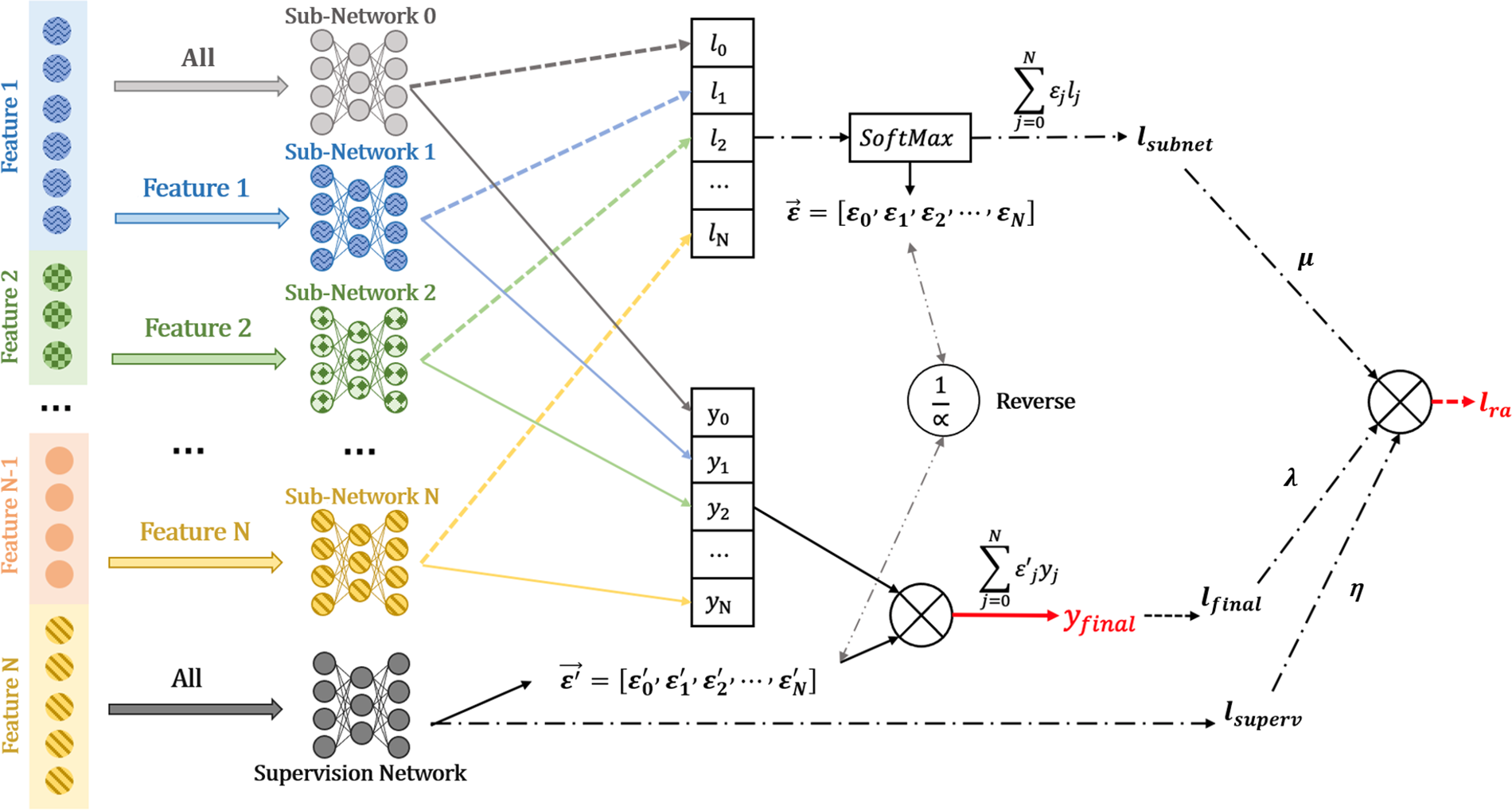
Figure 2: Structure of loss aware feature attention mechanism (LAFAM)

Specifically, we set up several sub-networks to learn the features, and the number and type of sub-networks can be adjusted according to different problems. The sub-networks shown in Fig. 2 are of different types. In our model, the output of each network is a score between 0 and 1, which indicates the sample’s probability of becoming a hot sale product learning within each respective network. A score of 0 signifies the lowest potential to be a hot sale product, and a score of 1 signifies the highest potential.

For each sub-network, the larger the loss value the lower the confidence of the current output. It is difficult to judge a sub-network based on features with low confidence, and these are usually discarded by the traditional methods. However, any feature will have an impact on the prediction result, and we should not discard a feature that is difficult to judge or makes a small contribution. For example, in e-commerce recommendations, commission, and rebate characteristics are often difficult to judge by the predictive network, but they are important. In our network, confidence means that the network should strengthen the learning of the sub-network, so its loss value accounts for a larger proportion of the loss of the entire network. Therefore, we calculate the softmax value of the loss value output by the network by Eq. (1), and determine the proportion of its contribution to the overall loss. At the end of the network, the weighted sum of the loss values obtains the overall loss.

For a given li,i∈(0,1,2,…,N), which is the output loss of sub-networks, we estimate the probability p(ε=j|li) for each category j with softmax, i.e., we estimate the probability of each classification result of ε. Let ε→=[ε0,ε1,ε2,…,εN] be a vector of weights of output values from each network. When we obtain the predicted value through the network, we hope that a result with high confidence will dominate. Therefore, in calculating the predicted value, we use the opposite coefficient εi as the weight of output from sub-networks:

εi=eli∑n=0NelN=eliel0+el1+⋯+elN,i=0,1,2,…,N(1)

Then, we design a supervised network whose output is the ratio of each subnetwork output to the total output. The labels used for training are the weight vectors ε′→=[ε1′,ε2′,ε3′,…,εN′] about li obtained after a softmax calculation based on the loss values. We substitute the parameters shown in Fig. 2 in the formula, which simplifies the ratio of each category to:

εi′=e−li∑n=0Ne−lN=e−lie−l0+e−l1+⋯+e−lN,i=0,1,2,…,N(2)

In the training process, we need to fit ε′→ and ε→ to make these two probability distributions infinitely close. Therefore, the final loss function lra is:

lra=λlfinal+μlsubnet+ηlsuperv=λ∥yfinal−y0∥2+με→∥ysubnet−y0∥2+η∥ysuperv→−ε′→∥2=λ∥yfinal−y0∥2+μ∑j=0NeljT⋅∥yj−y0∥2∑k=0NelkT+η∑j=0N∥ysuperv→−(1−elj∑k=1Nelk)∥2(3)

where λ, μ, and η are network parameters that can be set and adjusted using grid search or other tuning methods; yfinal is the final output of the network overall; y0 is the label of the original sample; ysubnet={y1,y2,…,yN} is the output of the sub-network; ysuperv→ is the output of the supervision network; N is the number of feature groups, which in this task is 4; and T is the temperature coefficient used in softmax operation, and it can adjust the difference between the values calculated by softmax.

In general, T≥1. The smaller T is, the steeper the softmax curve is, and the bigger the difference between the output values will be. The larger T is, the smoother the softmax curve is, and the difference between the output values will be small. In this way, we control the balance of weighting the sub-network loss li by the coefficient T.

3.3 Suppression Loss

We propose suppression loss to solve the class imbalance issue, which influences machine learning algorithms to classify inputs in the positive (majority) class every time to achieve high prediction accuracy. If we train the deep learning model with traditional loss functions (e.g., square loss, log loss), the loss value of positive samples will account for a larger proportion of the total loss. However, in practice, we are often more concerned with the accuracy of the negative class (precision or F-measure). For example, in our scenario, hot sale products are a minority, but traditional deep learning-based models tend to neglect the minority class and output general products as the prediction result. Therefore, regarding class imbalance, we want negative classes to contribute more loss value. Hence, we propose suppression loss:

Lsp(yfinal,y0)=[α(yfinal+β)2+2α(yfinal+β)+12]×[θ(|yfinal−y0|+ρ)2+2θ||yfinal−y0|+ρ|+12]×|yfinal−y0|γ(4)

where |yfinal−y0| is the absolute difference between the estimated probability yfinal and its true label y0; α, β, θ, ρ, and γ are the parameters of the model, which can be set according to the practical dataset problem through the grid search method.

The suppression loss function consists of three parts. The first part is the suppression of the loss contribution to the large category of samples through a function. The second part is to suppress the easy sample contribution by using the same function and different parameters. The last part is the suppression of the easy sample contribution employing a high-power function that expands the output disparity. The feasibility of suppression loss is explained below, and a more detailed process can be found in the Appendix (Figs. A1 and A2).

Firstly, we need a function fsp(x) to meet the following conditions:

•   The value range of fsp(x) is (0,1) or (0,1].

•   fsp(x)→0 when x→0. fsp(x)→1 when x→∞.

•   The function fsp(x) is continuous and differentiable.

We find that the simple function f(x)=x1+|x| has the above properties. This is an S-type function, with similar properties to a sigmoid function. However, f(x) is more concise and less complex, as shown in Fig. 3a. The function fsp(x)=α(x+β)2+2α|x+β|+12 is obtained by linear transformation (translation and compression). Its value range is (0,1), and its slope and the point over 0.5 can be adjusted by changing α and β. Fig. 3a is the original graph of f(x)=x1+|x|. Fig. 3b is a function diagram for controlling both the independent and dependent variables within the range of 0–1 after compression and translation. Fig. 3c is a graph of fsp(x) under different parameters, from which it can be seen that the larger α is, the larger the slope is, i.e., easily classified data can be better penalized. Fig. 3d is a comparative diagram of three loss function adjustment factors. When x is closer to 0, the smaller the suppression loss the stronger the penalty of easily classified data. The larger x is, the closer the function value is to 1. The function hardly punishes sufficiently large x. It can be seen from Fig. 3d that focal loss still inhibits large x values. The two-parameter control of shrinkage loss is not as accurate as the three-parameter control of suppression loss. Suppression loss has a simpler functional form than shrinkage loss (fsp(⋅) is simple, but fshrinkage(⋅) is elementary), which will greatly help its stability. We provide verification results in the following experiment.

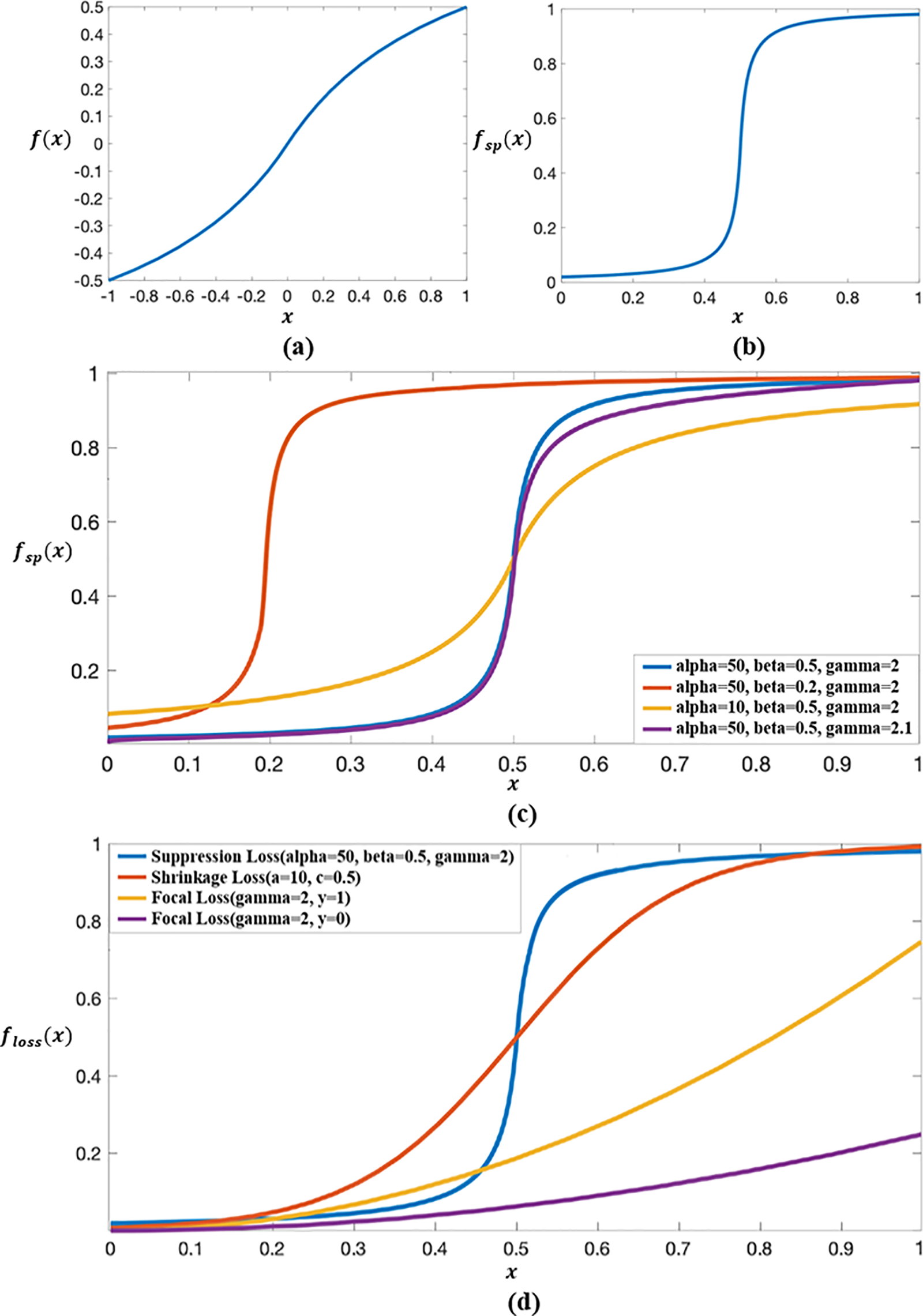
Figure 3: Proposed process of suppression loss: (a) The original graph of function f(x); (b) The graph of function after compression and translation; (c) The graph of fsp(x) under different parameters; (d) The comparative diagram of three loss function adjustment factors

When applied to classification problems, it is assumed that the label of the positive class is 0. In this case, the closer the predicted value is to 0, the more its loss is penalized, i.e., this kind of sample contributes less to the overall loss. If the label is 1, then the smaller the predicted value the larger its loss, and the less it is penalized in the function, so this kind of sample contributes greatly to the overall loss.

According to the focal loss [20], we superimpose fsp(⋅) on lγ. In this way, we can penalize the sample points of positive and easy classes. As shown in Table 1, easy positive sample points are penalized by fsp(⋅) and γ at the same time, i.e., they are restrained to the greatest extent. Hard positive sample points are penalized by fsp(⋅). Easy negative sample points are penalized by γ, while hard negative sample points are barely penalized. This achieves the goal of making hard negative sample points contribute the most loss. The accuracy of the classification of hard negative sample points determines the final loss value of the network. The more mistakes in hard negative sample points, the greater the loss. The network pays more attention to hard negative sample points. Therefore, the classification rate of negative classes can be improved.

4  Experiments

4.1 Datasets

We use the Tmall (Taobao) non-public dataset and the Kaggle public dataset Corporación Favorita Grocery Sales Forecasting (CFGSF) for experimental verification.

•   Tmall: The dataset is 10.7 GB in size and contains 51,134,193 rows of data, with 453 data features from August 2019 to August 2020. The dataset contains information such as product name, product category, product price, coupon price, historical sales volume, highest single-day sales, and single-day average sales.

•   CFGSF: It provides the sales information of 54 stores in different parts of Ecuador from 01 January 2013, to 31 August 2017, including commodity serial number, sales volume, and category; whether goods are easily corrupted; and whether they are in promotion. The dataset al.so provides the store category, city, total sales, and oil price on the day of the sale.

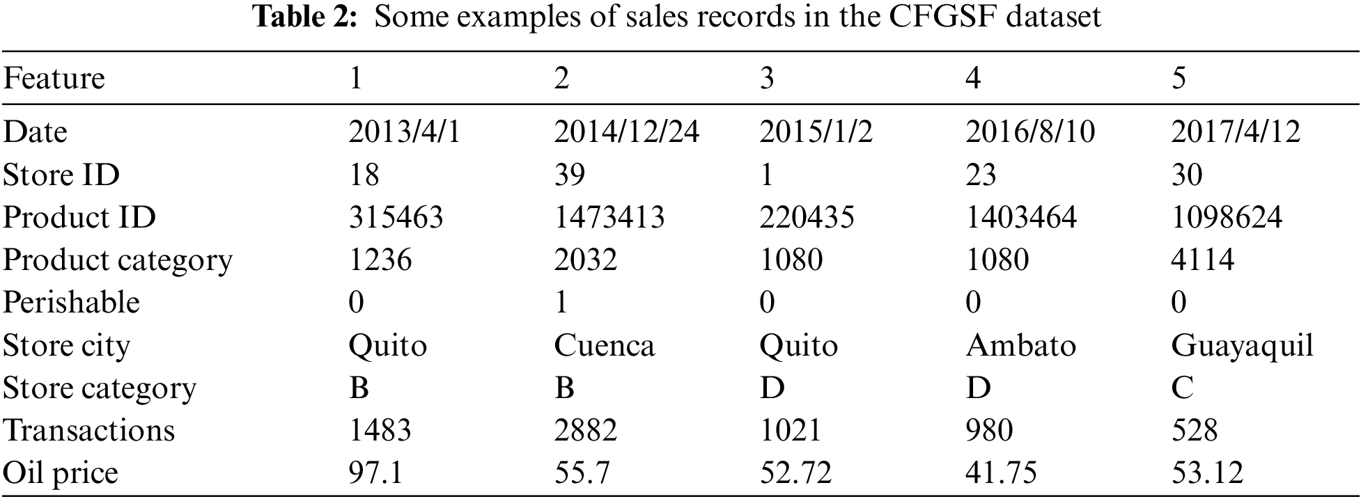
Table 2 presents some examples of sales records from the CFGSF dataset. After merging, extracting, cleaning, and screening to ensure that abnormal data and noise would not affect the classification accuracy of the neural network, the dataset contains 70,205,249 rows of data with a dataset size of 13.93 GB. To put the forecasting problem into practice, we transform the forecasting of commodity sales from a regression problem to a classification problem. After normalizing the sales volume of the training set, we select 0.15 as the threshold to define the two classifications. After classification, the data volumes of categories 0 and 1 are 70,184,766 and 20,483, respectively, and the imbalance ratio is 3426:1.

4.2 Structure and Parameter Settings of LAFAM

With a simple MoE structure, the importance weight distribution of the softmax gate learning model on experts of different feature groups is shown in Fig. 4a. The weight of time series features is high, followed by the importance of commission and voucher features. This is consistent with the conclusion from the PS-smart that the future sales volume of most samples is highly correlated with the sales volume of N days in recent history. Fig. 4b shows the learning result based on LAFAM. It has a high learning fit for a large number of simple samples, with high importance of historical time series features and insufficient learning of other features. We observe that the latter’s dependence weight distribution on different features is more even so that other basic feature models can also be fully learned, thereby obtaining better recommendation results.

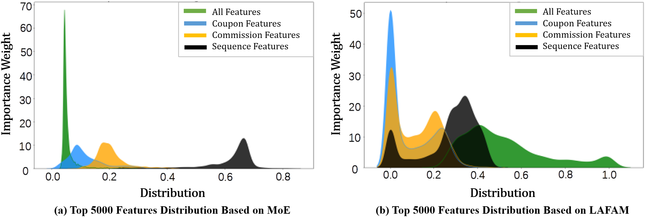
Figure 4: Importance weight distribution of different feature groups based on: (a) Simple mixture-of-experts (MoE) network; (b) Loss aware feature attention mechanism (LAFAM)

Therefore, in the process of realizing the model, we divide the features into four parts. The model application structure diagram is shown in Fig. 5. The basic feature depicts the basic attributes of commodities (including historical prices, historical sales, and other statistical features). The second and third parts are the coupling and commission features, which are the key factors to describe whether goods can become hot sale products. The fourth part is the sequence feature, i.e., the time series of daily transactions of commodities in the past three months. The features are categorized and fed into four distinct sub-networks.

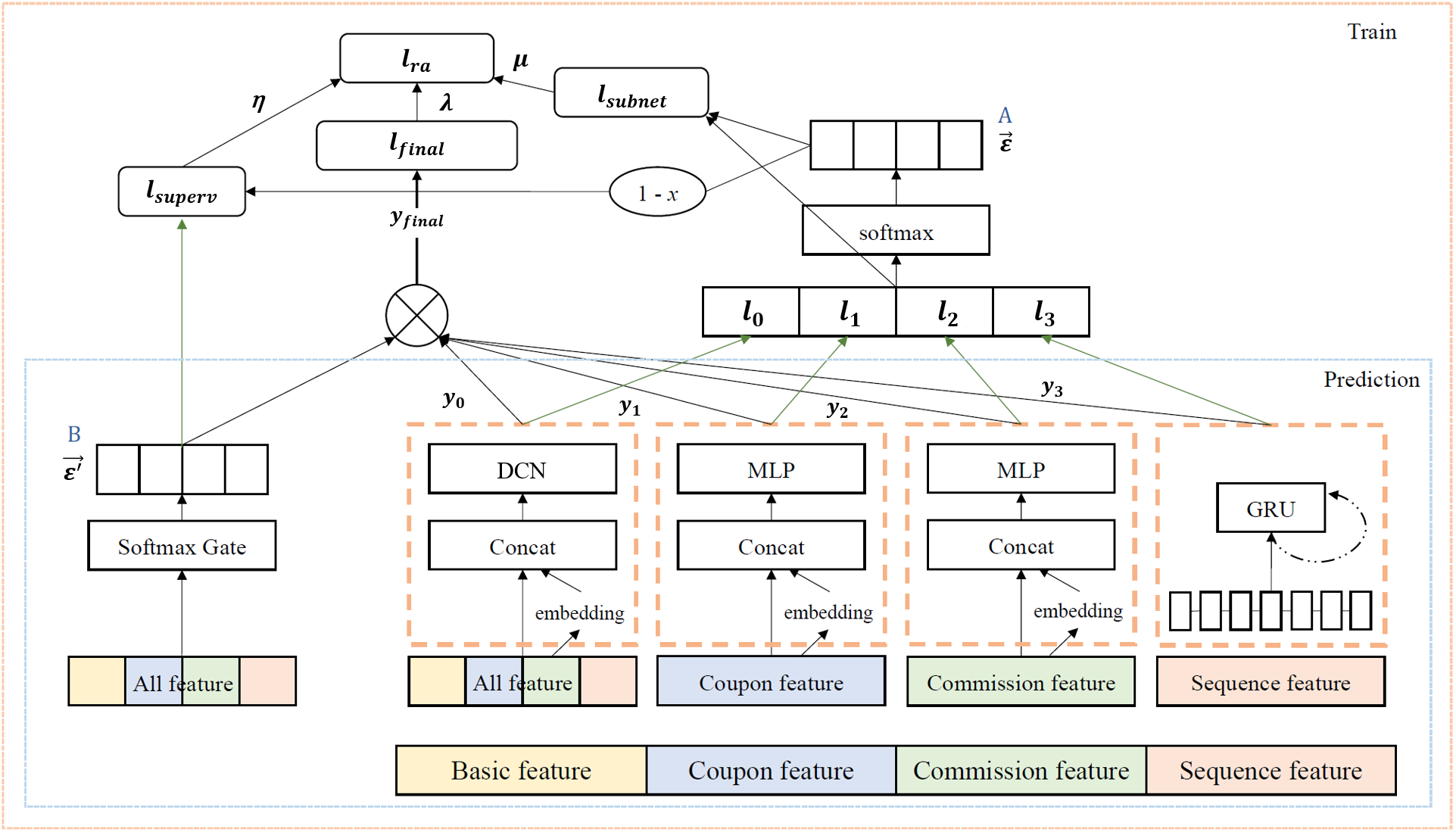
Figure 5: Application structure of our LAFAM

All features are processed using the deep & cross network (DCN), a commonly employed approach in recommendation systems, which includes 3 deep layers with ReLU activation functions and 2 cross layers. The cross layers are specifically designed to learn feature interactions in a more efficient manner, capturing bounded-degree interactions between features at different levels. This structure is highly effective for both vertical recommendations and wide-ranging interest exploration, and it offers high computational efficiency, making it an ideal choice for learning from all features. Coupling and commission features are handled using a 3-layer MLP with ReLU activation function, which can extract high-dimensional features from the samples, making it suitable for recommendation predictions. Sequence features are processed using a 2-layer gated recurrent unit (GRU), each layer with 64 hidden units and using the tanh activation function. The GRU is a variant of the long short-term memory (LSTM) network, itself an evolved form of the RNN, known for its excellent predictive performance. Compared to the LSTM, the GRU has a simpler structure and effectively addresses the long-term dependency problem of RNNs. This results in high computational efficiency and excellent accuracy, making the GRU well-suited for learning from sequence features. For the training process, we employ the Adam optimizer with a learning rate of 0.01 and a batch size of 64. The model is trained for 50 epochs, with the suppression loss used to compute the final loss value. The parameter settings for the LAFAM framework are determined based on our own experimental results to ensure optimal performance for the given dataset and task.

Combined with the theoretical derivation and practical application, we improve and optimize the network as follows:

•   We combine the idea of MoE to build an expert network for different feature groups. We combine the expert results through the softmax gate layer and use the loss aware method for learning. In the training process, the output result yi of each expert is calculated with the true value of loss in the training stage, which is recorded as l0, l1, l2, l3, and the distribution of different losses is obtained through a softmax layer. Assuming that each expert learns well and tries to accurately predict the final value yfinal, the distribution of loss represents the importance of different feature groups to the prediction results. Therefore, the difference in attention results of samples in different feature groups is strengthened in the training stage.

•   Because we cannot obtain the loss value of each part in the prediction stage, we add lsuperv in the training stage to measure the distance between the output probability distributions at A and B in Fig. 5. We make the probability distributions of two places similar.

•   MoE has disadvantages. It cannot guarantee that every sub-network in the framework will do its best to predict. Simply calculating the prediction results according to the smaller the loss the higher the weight will cause the model to gradually abandon the learning of the expert for the larger loss. This causes each expert to not do its best to predict the result, and it cannot reflect the authenticity of each expert’s attention result. Therefore, we propose lsubnet and lra. In the process of fusion, we pay more attention to the learning of the higher part of the loss, and control the balance of the softmax result through the temperature parameter T, so that each expert tries best to learn.

4.3 Evaluation Process and Metrics

We evaluate the performance of the LAFAM network, suppression loss, and the RS by controlling variables, as shown in Fig. 6. We first assess the performance of LAFAM according to regression problems. Since the output of LAFAM is a score (as shown in Fig. 1), which belongs to [0,1], the higher the score, the more likely a product is to become a hot sale product. Then, we use the parameters obtained through a grid search to verify the performance of suppression loss, and we validate the performance of LAFAM and suppression loss from a classification problem perspective. Finally, we verify the effect of the entire RS, i.e., the fusion of LAFAM and suppression loss.

Figure 6: Recommendation system (RS) evaluation process and result guidance

In the experiments, our proposed LAFAM can calculate the probability of a product being a hot sale product. In regression problems, the performance of LAFAM is assessed with four evaluation metrics, which are Root Mean Squared Error (RMSE), Mean Absolute Error (MAE), Weighted Mean Absolute Percentage Error (WMAPE), and Top 50/100/200 Hit Rate (HR@50/100/200). In sorting problems, we use Precision, Accuracy, and F-measure to evaluate the effectiveness of LAFAM and suppression loss.

RMSE presents the gap between the predicted value by the model and the true value:

RMSE=1n∑i=1n|y^i−yi|(5)

where n is the number of samples, y^i is the predicted output, and yi is the true label.

MAE directly calculates the absolute value of the error between the predicted value and the true value:

MAE=1n∑i=1n|y^i−yi|(6)

WMAPE weights the prioritized products so as to bias the prediction error towards those products:

WMAPE=∑i=1n|y^i−yi|∑i=1nyi(7)

HR is a recall-based metric, which is defined as:

HR@k=NkGT(8)

where GT denotes the number of test sets, and Nk denotes the sum of test sets in each user’s Top k recommended products.

Accuracy indicates the percentage of the number of correctly categorized samples to the total number of samples:

Accuracy=TP+TNTP+TN+FP+FN(9)

where TP indicates that the final prediction of the positive sample is positive, TN demonstrates that the final prediction of the negative sample is negative, FP means that the negative sample ends up with a positive prediction, FN implies that the positive sample ends up with a negative prediction.

Precision denotes the proportion of correctly categorized positive samples out of all categorized positive samples:

Precision=TPTP+FP(10)

Recall represents how many of all positive samples are correctly categorized by the model. F-measure is the harmonic mean of Precision and Recall:

Recall=TPTP+FN(11)

F−measure=(1+β2)×Recall×Precisionβ2×Recall+Precision(12)

where β is a coefficient regulating the weight of Precision and Recall, typically taken as 1.

4.4 Results

4.4.1 Regression Validation of LAFAM

To verify the performance improvement of the LAFAM network, we first compare the model with the following models widely used in recommendation systems in terms of a regression problem:

•   GBDT (Gradient Boosting Decision Tree) [64]: an ensemble learning method that builds and combines many decision trees sequentially to improve predictive performance by minimizing errors.

•   DCN (Deep & Cross Network) [65]: it retains the benefits of the deep neural network and introduces a novel cross network to learn certain bounded-degree feature interactions more efficiently.

•   MoE (Mixture-of-Experts) [30]: it consists of several feed-forward sub-networks and selects a sparse combination of sub-networks via a trainable gated network.

In this experiment, the squared loss function is used as the basic backpropagation loss function. For GBDT, we use a learning rate of 0.1, a maximum depth of 6, and 100 boosting iterations. For DCN, we follow a standard configuration with 3 deep layers and 2 cross layers, utilizing ReLU as the activation function. For MoE, we configured the model with 4 experts and 2 gating layers, with each expert being an MLP with 3 hidden layers. These settings are selected based on both previous studies and a hyperparameter tuning process conducted in our own experiments to ensure all models were optimized under the same conditions.

On the model side, MAE can intuitively show the regression error situation, RMSE can better reflect the influence of extreme values on the error, while WMAPE is less affected by extreme values and individuals, and can show the overall prediction of the network more evenly. Therefore, the three metrics together can measure the performance of the regression model more completely. However, since the prediction problem in this paper is a class imbalance problem, the metrics above are all calculated with the same weights for both large and small classes, so they cannot well reflect the effectiveness of the network for the imbalance problem. For this reason, we choose the metric HR@K to judge the performance of the model under imbalance conditions in practical application.

The experimental results as regression problems are shown in Table 3. It shows that LAFAM outperforms other network structures on both datasets. In terms of RMSE, MAE, and WMAPE, the LAFAM network has no obvious disadvantage compared with other networks, and even if it cannot reach the best, it is still very close to the best value. Moreover, MAE and WMAPE parameters even occupy the optimal position in the Tmall dataset. RMSE parameters are reduced because large classes contribute many loss values in highly unbalanced datasets. In practical applications, we often measure the performance of a model by HR@K (K = 50, 100, 200), the hit rate of the top K products. It can be seen from Table 2 that LAFAM improves stability on the HR@K parameter. For the Tmall dataset, LAFAM increases by 34.8%, 8.4%, and 10.4% on HR@50, HR@100 and HR@200, respectively, compared to MoE. For the CGFSF dataset, the improvement is 22.9%, 3.6%, and 24.4%, respectively. This is a great benefit in practical commercial applications. It indicates that LAFAM can optimize the problem of reduced prediction accuracy caused by feature imbalance and class imbalance, and has certain advantages compared to other recommendation applications.

4.4.2 Classification Validation of LAFAM and Suppression Loss

In practical applications, conspicuous positions on the sales page are limited, so we require high prediction accuracy. We can accept the misclassification of small categories into large categories, but the misclassification of large categories into small categories is costly and unacceptable. Therefore, in the experiment, the higher the precision the better the experimental effect. We also refer to the F-measure and accuracy to comprehensively evaluate the network. The F-measure is a typical parameter to measure the effect of a model in an unbalanced data field.

We determine the parameters of suppression loss function by grid search. Fig. 7 shows the grid search process of suppression loss, where the red dot position is the selected parameter value, and other experiments are conducted in the same way. Since the practical tuning uses high dimensions for the search, the location of the red point in Fig. 7b is not the global optimal solution, but it has optimal performance when combined with other parameters. The optimal parameter points are selected as experimental parameters, whose final values are shown in Table 4.

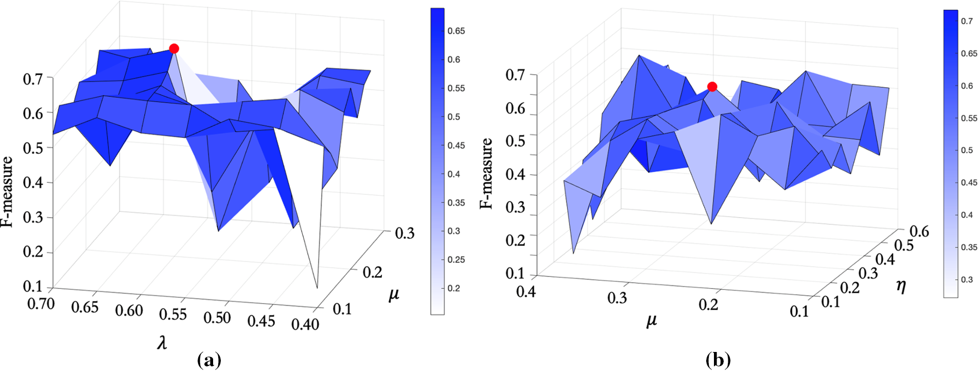
Figure 7: Suppression loss grid search image: (a) λ and μ; (b) μ and η

We should ensure the stability of the function as well as its effectiveness. Fig. 8 shows the change curves of accuracy and loss during training with shrinkage and suppression loss, from which we can find that acc and loss values of suppression loss basically do not fluctuate after reaching a stable level. In addition, there is obviously less gradient disappearance and explosion of suppression loss during training, so its performance is more stable. Stable performance will have higher credibility in practical application, which also benefits recommendation income.

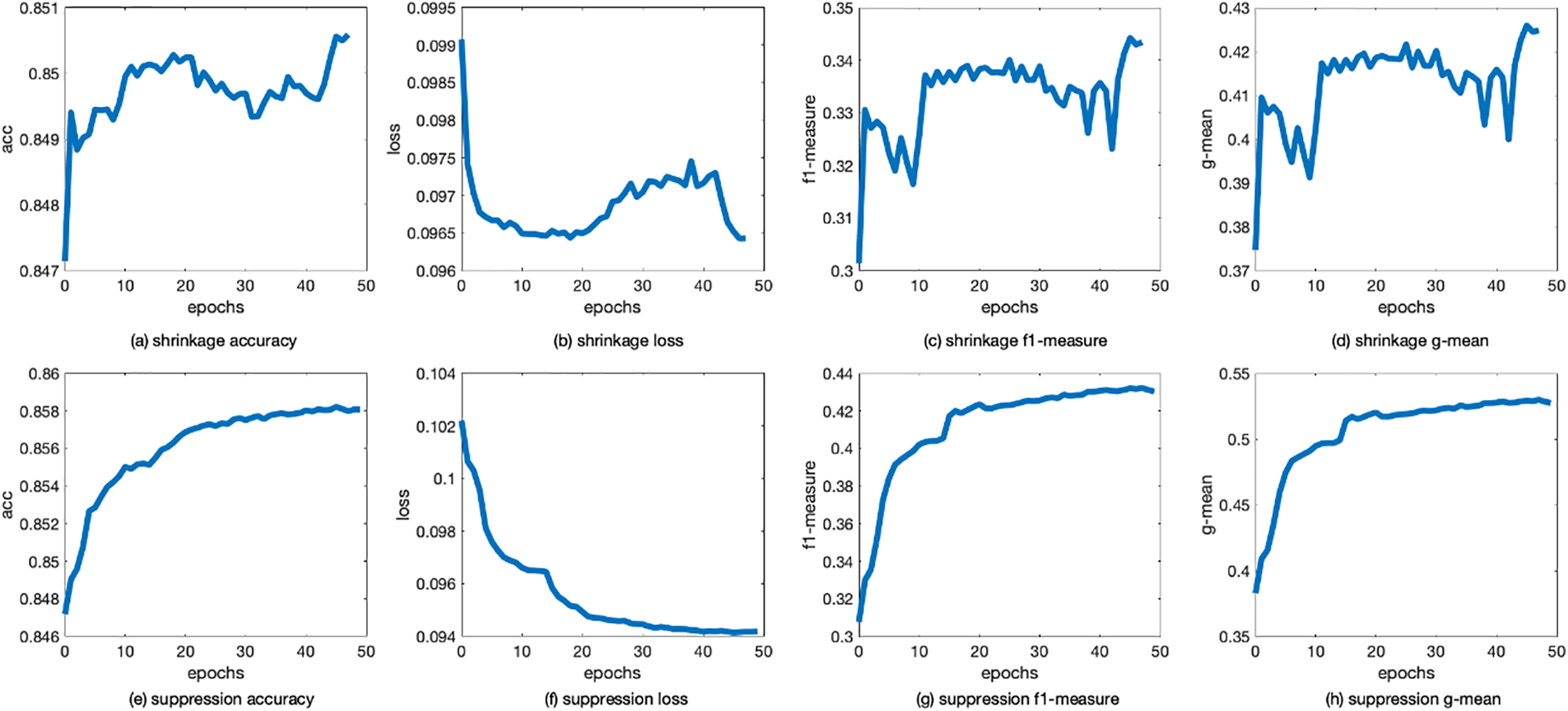
Figure 8: Comparison of training process between shrinkage loss and suppression loss

Since both LAFAM and suppression loss have excellent performance in the control variable test, we use them together to verify the effectiveness of the RS for class and feature imbalance. We examine focal loss, shrinkage loss, and suppression loss respectively under different networks, and select MLP, GRU, DCN, MoE, and LAFAM networks for comparison. The first four are the sub-networks used in the LAFAM network in this paper and thus are tested separately. The parameter settings of the sub-networks used for comparison are kept consistent with the LAFAM network. In this way, we complete the ablation experiment while baseline comparison, proving that the joint network has enhancement compared to each sub-network.

Table 5 shows the performance of loss functions in different networks based on the imbalanced dataset Tmall. The imbalance ratios of 1:5, 1:10, and 1:20 are selected to represent different levels of data imbalance commonly observed in real-world recommendation system applications. These ratios simulate different degrees of data skewness, allowing us to evaluate the performance of the LAFAM network and suppression loss under both mild (1:5) and extreme (1:20) imbalance conditions. By testing across these imbalance degrees, we ensure the generalizability of our findings across different levels of class distribution imbalances that are relevant in practical applications.

Regarding the network, LAFAM shows significant improvements on the dataset with a high imbalance degree compared to the other networks. In the 1:20 imbalance dataset, the LAFAM is in the optimal position for all three parameters, which is about 10% higher than the other networks on average. While in the 1:5 and 1:10 imbalance datasets, it is only about 7% lower than the optimal network on average. Therefore, the LAFAM network is used in the class imbalance and feature imbalance datasets with stable results and obvious advantages. Regarding the loss function, it can be found that suppression loss has better performance in each network, as it can well solve the problems of the unbalanced number of categories and unbalanced sample discriminant confidence. The experimental results of the suppression loss have an average increase of about 15% compared to the other loss functions, which shows that it has good adaptability to unbalanced datasets. The LAFAM-suppression loss, which is combined with the two methods, has the best performance under a 1:20 imbalance degree (which is closest to practical application). The performance superiority of LAFAM-suppression loss continues to increase with the imbalance ratio. Therefore, it can be concluded that LAFAM-suppression loss can improve the recommendation of multi-angle imbalance.

5  Conclusion and Future Work

We proposed an RS to solve the recommendation problem on unbalanced datasets. It includes the LAFAM network framework and suppression loss, which can solve the issues of feature and class imbalance, respectively. Combined, they can well improve the imbalance issue encountered in the traditional machine learning algorithm used in the RS field. Comparative experiments using other networks and loss functions on two datasets show that they can solve the imbalance issue. Furthermore, the results on datasets with a high degree of imbalance show greater improvement than traditional methods.

For future work, our proposed LAFAM network requires background data to make recommendations, and thus cannot cope with the cold-start issue. We can optimize this problem by fast trial or interest migration. Alternatively, supervised learning can be combined with reinforcement learning to promote recommendation accuracy, diversity, and vertical category ratio optimization for unbalanced e-commerce data.

Acknowledgement: We sincerely thank Zhenyu Zhang of Alibaba Group for providing the dataset for this study.

Funding Statement: This work was supported by the National Key Research and Development Program of China (Grant numbers: 2021YFF0901705, 2021YFF0901700); the State Key Laboratory of Media Convergence and Communication, Communication University of China; the Fundamental Research Funds for the Central Universities; the High-Quality and Cutting-Edge Disciplines Construction Project for Universities in Beijing (Internet Information, Communication University of China).

Author Contributions: Conceptualization, Yuewei Wu; Methodology, Yuewei Wu, Ruiling Fu; Data curation, Ruiling Fu, Tongtong Xing; Formal analysis, Ruiling Fu, Tongtong Xing; Investigation, Yuewei Wu, Fuliang Yin; Writing—original draft, Yuewei Wu, Ruiling Fu. All authors reviewed the results and approved the final version of the manuscript.

Availability of Data and Materials: Due to the nature of this research, participants of this study did not agree for their data to be shared publicly, so supporting data is not available.

Ethics Approval: Not applicable.

Conflicts of Interest: The authors declare no conflicts of interest to report regarding the present study.

References

1. L. Wu, X. He, X. Wang, K. Zhang, and M. Wang, “A Survey on accuracy-oriented neural recommendation: From collaborative filtering to information-rich recommendation,” IEEE Trans. Knowl. Data Eng., vol. 35, no. 5, pp. 4425–4445, May 2023. doi: 10.1109/TKDE.2022.3145690. [Google Scholar] [CrossRef]

2. N. Khan, Z. Ma, A. Ullah, and K. Polat, “Categorization of knowledge graph based recommendation methods and benchmark datasets from the perspectives of application scenarios: A comprehensive survey,” Expert Syst. Appl., vol. 206, no. 15, Nov. 2022, Art. no. 117737. doi: 10.1016/j.eswa.2022.117737. [Google Scholar] [CrossRef]

3. Y. Wang, W. Ma, M. Zhang, Y. Liu, and S. Ma, “A Survey on the Fairness of Recommender Systems,” ACM Trans. Inf. Syst., vol. 41, no. 3, Feb. 2023, Art. no. 52. doi: 10.1145/3547333. [Google Scholar] [CrossRef]

4. S. Dhelim, N. Aung, M. A. Bouras, H. Ning, and E. Cambria, “A survey on personality-aware recommendation systems,” Artif. Intell. Rev., vol. 55, no. 3, pp. 2409–2454, Mar. 2022. doi: 10.1007/s10462-021-10063-7. [Google Scholar] [CrossRef]

5. R. E. Bawack, S. F. Wamba, K. D. A. Carillo, and S. Akter, “Artificial intelligence in e-commerce: A bibliometric study and literature review,” Electr. Mark., vol. 32, pp. 297–338, Mar. 2022. doi: 10.1007/s12525-022-00537-z. [Google Scholar] [PubMed] [CrossRef]

6. Y. Bai and H. Li, “Mapping the evolution of e-commerce research through co-word analysis: 2001–2020,” Electr. Commer. R. A., vol. 55, no. 2, Sep.–Oct. 2022, Art. no. 101190. doi: 10.1016/j.elerap.2022.101190. [Google Scholar] [CrossRef]

7. C. Pei et al., “Value-aware recommendation based on reinforcement profit maximization,” in World Wide Web Conf. (WWW’19), San Francisco, CA, USA, May 13–17, 2019, pp. 3123–3129. [Google Scholar]

8. B. Zhou and T. Zou, “Competing for recommendations: The strategic impact of personalized product recommendations in online marketplaces,” Market. Sci., vol. 42, no. 2, pp. 360–376, Mar.–Apr. 2023. doi: 10.1287/mksc.2022.1388. [Google Scholar] [CrossRef]

9. E. Gómez, L. Boratto, and M. Salamó, “Provider fairness across continents in collaborative recommender systems,” Inform. Process. Manag., vol. 59, no. 1, Jan. 2022, Art. no. 102719. doi: 10.1016/j.ipm.2021.102719. [Google Scholar] [CrossRef]

10. G. Aguiar, B. Krawczyk, and A. Cano, “A survey on learning from imbalanced data streams: Taxonomy, challenges, empirical study, and reproducible experimental framework,” Mach. Learn., vol. 113, pp. 4165–4243, Jun. 2024. doi: 10.1007/s10994-023-06353-6. [Google Scholar] [CrossRef]

11. Y. Zhu, Y. Geng, Y. Li, J. Qiang, Y. Yuan and X. Wu, “Self-adaptive deep asymmetric network for imbalanced recommendation,” IEEE Trans. Emerg. Top. Comput. Intell., vol. 8, no. 1, pp. 968–980, Feb. 2024. doi: 10.1109/TETCI.2023.3300740. [Google Scholar] [CrossRef]

12. X. Zhang, R. Li, B. Zhang, Y. Yang, J. Guo and X. Ji, “An instance-based learning recommendation algorithm of imbalance handling methods,” Appl. Math. Comput., vol. 351, pp. 204–218, Jun. 2019. doi: 10.1016/j.amc.2018.12.020. [Google Scholar] [CrossRef]

13. L. Yu et al., “A biased sampling method for imbalanced personalized ranking,” in Proc. 31st ACM Int. Conf. Inform. Knowl. Manag. (CIKM’22), Atlanta, GA, USA, Oct. 17–21, 2022, pp. 2393–2402. [Google Scholar]

14. M. Kim, Y. Yang, J. H. Ryu, and T. Kim, “Meta-learning with adaptive weighted loss for imbalanced cold-start recommendation,” in Proc. 32nd ACM Int. Conf. Inform. Knowl. Manag. (CIKM’23), Birmingham, UK, Oct. 21–25, 2023, pp. 1077–1086. [Google Scholar]

15. Y. Qiao, Y. Wu, F. Duo, W. Lin, and J. Yang, “Siamese neural networks for user identity linkage through web browsing,” IEEE Trans. Neural Netw. Learn. Syst., vol. 31, no. 8, pp. 2741–2751, Aug. 2020. doi: 10.1109/TNNLS.2019.2929575. [Google Scholar] [PubMed] [CrossRef]

16. K. Oksuz, B. C. Cam, S. Kalkan, and E. Akbas, “Imbalance problems in object detection: A review,” IEEE Trans. Pattern Anal. Mach. Intell., vol. 43, no. 10, pp. 3388–3415, Oct. 2021. doi: 10.1109/TPAMI.2020.2981890. [Google Scholar] [PubMed] [CrossRef]

17. G. Wang, Q. Song, H. Sun, X. Zhang, B. Xu and Y. Zhou, “A feature subset selection algorithm automatic recommendation method,” J. Artif. Intell. Res., vol. 47, pp. 1–34, May 2013. doi: 10.1613/jair.3831. [Google Scholar] [CrossRef]

18. E. H. Han and G. Karypis, “Feature-based recommendation system,” in Proc. 14th ACM Int. Conf. Inform. Knowl. Manag. (CIKM’05), Bremen, Germany, Oct. 31–Nov. 05, 2015, pp. 446–452. [Google Scholar]

19. Y. Wu, W. Zhang, L. Zhang, Y. Qiao, J. Yang and C. Cheng, “A multi-clustering algorithm to solve driving cycle prediction problems based on unbalanced data sets: A Chinese case study,” Sensors, vol. 20, no. 9, Apr. 2020, Art. no. 2448. doi: 10.3390/s20092448. [Google Scholar] [PubMed] [CrossRef]

20. T. Y. Lin, P. Goyal, R. Girshick, K. He, and P. Dollár, “Focal loss for dense object detection,” IEEE Trans. Pattern Anal. Mach. Intell., vol. 42, no. 2, pp. 318–327, Feb. 2020. doi: 10.1109/TPAMI.2018.2858826. [Google Scholar] [PubMed] [CrossRef]

21. X. Lu, C. Ma, B. Ni, X. Yang, I. Reid and M. H. Yang, “Deep regression tracking with shrinkage loss,” in Comput. Vis.-ECCV 2018: 15th European Conf., Munich, Germany, Sep. 08–14, 2018, pp. 369–386. [Google Scholar]

22. S. Park, Y. Hong, B. Heo, S. Yun, and J. Y. Choi, “The majority can help the minority: Context-rich minority oversampling for long-tailed classification,” in Proc. 2022 IEEE/CVF Conf. Comput. Vis. Pattern Recognit. (CVPR’22), New Orleans, LA, USA, Jun. 18–24, 2022, pp. 6877–6886. [Google Scholar]

23. S. Goyal, “Handling class-imbalance with KNN (neighbourhood) under-sampling for software defect prediction,” Artif. Intell. Rev., vol. 55, pp. 2409–2454, Mar. 2022. doi: 10.1007/s10462-021-10044-w. [Google Scholar] [CrossRef]

24. H. Kaur, H. S. Pannu, and A. K. Malhi, “A systematic review on imbalanced data challenges in machine learning: Applications and solutions,” ACM Comput. Surv., vol. 52, no. 4, Aug. 2019, Art. no. 79. doi: 10.1145/3343440. [Google Scholar] [CrossRef]

25. A. N. Tarekegn, M. Giacobini, and K. Michalak, “A review of methods for imbalanced multi-label classification,” Pattern Recogn., vol. 118, Oct. 2021, Art. no. 107965. doi: 10.1016/j.patcog.2021.107965. [Google Scholar] [CrossRef]

26. T. Meng, X. Jing, Z. Yan, and W. Pedrycz, “A survey on machine learning for data fusion,” Inform. Fusion., vol. 57, pp. 115–129, May 2022. doi: 10.1016/j.inffus.2019.12.001. [Google Scholar] [CrossRef]

27. S. Ji, Z. Wang, T. Li, and Y. Zheng, “Spatio-temporal feature fusion for dynamic taxi route recommendation via deep reinforcement learning,” Knowl.-Based Syst., vol. 205, Oct. 2020, Art. no. 106302. doi: 10.1016/j.knosys.2020.106302. [Google Scholar] [CrossRef]

28. J. H. Wang, Y. T. Wu, and L. Wang, “Predicting implicit user preferences with multimodal feature fusion for similar user recommendation in social media,” Appl. Sci., vol. 11, no. 3, Jan. 2021, Art. no. 1064. doi: 10.3390/app11031064. [Google Scholar] [CrossRef]

29. L. Lin, Z. Xu, and Y. Nian, “FFDNN: Feature fusion depth neural network model of recommendation system,” in Proc. 2020 Int. Conf. Internet of Things Intell. Appl. (ITIA’20), Zhenjiang, China, Nov. 27–29, 2020, pp. 1–5. [Google Scholar]

30. N. Shazeer et al., “Outrageously large neural networks: The sparsely-gated mixture-of-experts layer,” 2017, arXiv:1701.06538. [Google Scholar]

31. J. M. Johnson and T. M. Khoshgoftaar, “Survey on deep learning with class imbalance,” J. Big Data, vol. 6, Mar. 2019, Art. no. 27. doi: 10.1186/s40537-019-0192-5. [Google Scholar] [CrossRef]

32. A. Bria, C. Marrocco, and F. Tortorella, “Addressing class imbalance in deep learning for small lesion detection on medical images,” Comput. Biol. Med., vol. 120, May 2020, Art. no. 103735. doi: 10.1016/j.compbiomed.2020.103735. [Google Scholar] [PubMed] [CrossRef]

33. H. Cang et al., “Jujube quality grading using a generative adversarial network with an imbalanced data set,” Biosyst. Eng., vol. 236, pp. 224–237, Dec. 2023. doi: 10.1016/j.biosystemseng.2023.11.002. [Google Scholar] [CrossRef]

34. E. Gómez, “Characterizing and mitigating the impact of data imbalance for stakeholders in recommender systems,” in Proc. 14th ACM Conf. Recommender Syst. (RecSys’20), Brazil, Sep. 22–26, 2020, pp. 756–757. [Google Scholar]

35. R. Qin, Z. Wang, S. Huang, and L. Huangfu, “MSTIL: Multi-cue shape-aware transferable imbalance learning for effective graphic API recommendation,” J. Syst. Software., vol. 200, Jun. 2023, Art. no. 111650. doi: 10.1016/j.jss.2023.111650. [Google Scholar] [CrossRef]

36. S. Dhote, C. Vichoray, R. Pais, S. Baskar, and P. Mohamed Shakeel, “Hybrid geometric sampling and AdaBoost based deep learning approach for data imbalance in e-commerce,” Electr. Commer. Res., vol. 20, no. 2, pp. 259–274, Jun. 2020. doi: 10.1007/s10660-019-09383-2. [Google Scholar] [CrossRef]

37. R. G. Wang, X. Zhang, Y. Gao, A. L. Yee, and X. Wang, “The use of an internet of things data management system using data mining association algorithm in an e-commerce platform,” J. Organ. End User Com., vol. 35, no. 3, pp. 1–19, May 2023. doi: 10.4018/JOEUC.322553. [Google Scholar] [CrossRef]

38. G. Wei, W. Mu, Y. Song, and J. Dou, “An improved and random synthetic minority oversampling technique for imbalanced data,” Knowl.-Based Syst., vol. 248, Jul. 2022, Art. no. 108839. doi: 10.1016/j.knosys.2022.108839. [Google Scholar] [CrossRef]

39. J. Hoyos-Osorio, A. Alvarez-Meza, G. Daza-Santacoloma, A. Orozco-Gutierrez, and G. Castellanos-Dominguez, “Relevant information undersampling to support imbalanced data classification,” Neurocomputing, vol. 436, pp. 136–146, May 2021. doi: 10.1016/j.neucom.2021.01.033. [Google Scholar] [CrossRef]

40. V. Werner de Vargas, J. A. Schneider Aranda, R. dos Santos Costa, P. R. da Silva Pereira, and J. L. Victória Barbosa, “Imbalanced data preprocessing techniques for machine learning: A systematic mapping study,” Knowl. Inf. Syst., vol. 65, no. 1, pp. 31–57, Jan. 2023. doi: 10.1007/s10115-022-01772-8. [Google Scholar] [PubMed] [CrossRef]

41. C. Lin, C. F. Tsai, and W. C. Lin, “Towards hybrid over-and under-sampling combination methods for class imbalanced datasets: An experimental study,” Artif. Intell. Rev., vol. 56, no. 2, pp. 845–863, Apr. 2022. doi: 10.1007/s10462-022-10186-5. [Google Scholar] [CrossRef]

42. A. Sze-To and A. K. C. Wong, “A weight-selection strategy on training deep neural networks for imbalanced classification,” in Image Anal. Recognit.: 14th Int. Conf. (ICIAR’2017), Montreal, QC, Canada, Jul. 05–07, 2017, pp. 3–10. [Google Scholar]

43. D. Tran, H. Mac, V. Tong, H. A. Tran, and L. G. Nguyen, “A LSTM based framework for handling multiclass imbalance in DGA botnet detection,” Neurocomputing, vol. 275, pp. 2401–2413, Jan. 2018. doi: 10.1016/j.neucom.2017.11.018. [Google Scholar] [CrossRef]

44. Y. Chen, B. Pang, G. Shao, G. Wen, and X. Chen, “DGA-based botnet detection toward imbalanced multiclass learning,” Tsinghua Sci. Technol., vol. 26, no. 4, pp. 387–402, Aug. 2021. doi: 10.26599/TST.2020.9010021. [Google Scholar] [CrossRef]

45. H. T. Lin, “Advances in cost-sensitive multiclass and multilabel classification,” in Proc. 25th ACM SIGKDD Int. Conf. Knowl. Discov. Data Min., Anchorage, AK, USA, Aug. 04–08, 2019, pp. 3187–3188. [Google Scholar]

46. Z. Wang et al., “An industrial framework for personalized serendipitous recommendation in E-commerce,” in Proc. 17th ACM Conf. Recommender Syst. (RecSys’23), Singapore, Sep. 18–22, 2023, pp. 1015–1018. [Google Scholar]

47. I. Islek and S. G. Oguducu, “A hierarchical recommendation system for E-commerce using online user reviews,” Electr. Commer. R. A, vol. 52, Mar.–Apr. 2022, Art. no. 101131. doi: 10.1016/j.elerap.2022.101131. [Google Scholar] [CrossRef]

48. S. Wei, Z. Wang, X. An, Q. Li, H. Xiao and Y. Xiao, “A recommendation model for e-commerce platforms oriented to explicit information compensation and hidden information mining,” Knowl.-Based Syst., vol. 286, Feb. 2024, Art. no. 111359. doi: 10.1016/j.knosys.2023.111359. [Google Scholar] [CrossRef]

49. Z. Movafegh and A. Rezapour, “Improving collaborative recommender system using hybrid clustering and optimized singular value decomposition,” Eng. Appl. Artif. Intel., vol. 126, Nov. 2023, Art. no. 107109. doi: 10.1016/j.engappai.2023.107109. [Google Scholar] [CrossRef]

50. K. Patel and H. B. Patel, “A state-of-the-art survey on recommendation system and prospective extensions,” Comput. Electron. Agr., vol. 178, Nov. 2020, Art. no. 105779. doi: 10.1016/j.compag.2020.105779. [Google Scholar] [CrossRef]

51. Y. Pérez-Almaguer, R. Yera, A. A. Alzahrani, and L. Martínez, “Content-based group recommender systems: A general taxonomy and further improvements,” Expert Syst. Appl., vol. 184, Dec. 2021, Art. no. 115444. doi: 10.1016/j.eswa.2021.115444. [Google Scholar] [CrossRef]

52. Y. Lu and Y. Duan, “Online content-based sequential recommendation considering multimodal contrastive representation and dynamic preferences,” Neural Comput. Appl., vol. 36, no. 13, pp. 7085–7103, Feb. 2024. doi: 10.1007/s00521-024-09447-x. [Google Scholar] [CrossRef]

53. Y. Koren, S. Rendle, and R. Bell, “Advances in collaborative filtering,” in Recommender Syst. Handbook, New York, NY, USA: Springer, Nov. 2021, pp. 91–142. doi: 10.1007/978-1-0716-2197-4_3. [Google Scholar] [CrossRef]

54. S. Sharma, V. Rana, and M. Malhotra, “Automatic recommendation system based on hybrid filtering algorithm,” Educ. Inf. Technol., vol. 27, pp. 1523–1538, Jul. 2021. doi: 10.1007/s10639-021-10643-8. [Google Scholar] [CrossRef]

55. Z. Z. Darban and M. H. Valipour, “GHRS: Graph-based hybrid recommendation system with application to movie recommendation,” Expert Syst. Appl., vol. 200, Aug. 2022, Art. no. 116850. doi: 10.1016/j.eswa.2022.116850. [Google Scholar] [CrossRef]

56. A. Da’u and N. Salim, “Recommendation system based on deep learning methods: A systematic review and new directions,” Artif. Intell. Rev., vol. 53, pp. 2709–2748, Apr. 2020. doi: 10.1007/s10462-019-09744-1. [Google Scholar] [CrossRef]

57. M. M. Islam, S. Nooruddin, F. Karray, and G. Muhammad, “Human activity recognition using tools of convolutional neural networks: A state of the art review, data sets, challenges, and future prospects,” Comput. Biol. Med., vol. 149, Oct. 2022, Art. no. 106060. doi: 10.1016/j.compbiomed.2022.106060. [Google Scholar] [PubMed] [CrossRef]

58. H. Hewamalage, C. Bergmeir, and K. Bandara, “Recurrent neural networks for time series forecasting: Current status and future directions,” Int. J. Forecasting., vol. 37, no. 1, pp. 388–427, Jan.–Mar. 2021. doi: 10.1016/j.ijforecast.2020.06.008. [Google Scholar] [CrossRef]

59. M. A. Chatti, M. Guesmi, and A. Muslim, “Visualization for recommendation explainability: A survey and new perspectives,” ACM T. Interact. Intel., vol. 14, no. 3, pp. 1–40, Aug. 2024. doi: 10.1145/3672276. [Google Scholar] [CrossRef]

60. C. Chen, A. D. Tian, and R. Jiang, “When post hoc explanation knocks: Consumer responses to explainable AI recommendations,” J. Interact. Mark., vol. 59, no. 3, pp. 234–250, Dec. 2023. doi: 10.1177/10949968231200221. [Google Scholar] [CrossRef]

61. R. Dwivedi et al., “Explainable AI (XAICore ideas, techniques, and solutions,” ACM Comput. Surv., vol. 55, no. 9, pp. 1–33, Jan. 2023. doi: 10.1145/3561048. [Google Scholar] [CrossRef]

62. M. Li et al., “Scaling distributed machine learning with the parameter server,” in Proc. 11th USENIX Conf. Oper. Syst. Design Implementation, Broomfield, CO, Oct. 06–08, 2014, pp. 583–598. [Google Scholar]

63. T. Chen and C. Guestrin, “XGBoost: A scalable tree boosting system,” in Proc. 22nd ACM SIGKDD Int. Conf. Knowl. Discov. Data Min., San Francisco, CA, USA, Aug. 13–17, 2016, pp. 785–794. [Google Scholar]

64. J. H. Friedman, “Greedy function approximation: A gradient boosting machine,” Ann. Stat., vol. 29, no. 5, pp. 1189–1232, Oct. 2001. [Google Scholar]

65. R. Wang, B. Fu, G. Fu, and M. Wang, “Deep & cross network for ad click predictions,” in Proc. ADKDD’17, Halifax, NS, Canada, Aug. 14, 2017, pp. 1–7. [Google Scholar]

Appendix A. Suppression Loss Feasibility Proof

A loss function must be continuous and differentiable in R. Therefore, we will prove the continuity and differentiability of Lsp, which requires us to prove that f(x)=x1+|x| is continuous and differentiable.

f(⋅) is a piecewise function. When x>0, f(x)=x1+x, and f(⋅) is obviously continuous and differentiable. When x<0, f(x)=x1−x, and again, f(⋅) is obviously continuous and differentiable. Therefore, we only need to prove that f(⋅) is continuous and differentiable at x=0.

We first prove that f(⋅) is differentiable at point 0.

f+(x)=x1+x(A1)

f−(x)=x1−x(A2)

f+′(x)=1+x−x(1+x)2=1(1+x)2(A3)

f−′(x)=1−x+x(1−x)2=1(1−x)2(A4)

When x=0, f+′(x)=f−′(x)=1. Therefore, f(⋅) is differentiable in the real domain.

We next prove that f(⋅) is continuous at 0.

f(0+)=limx→0+x1+x=limx→0+11x+1=0(A5)

f(0−)=limx→0−x1−x=limx→0+11x−1=0(A6)

f(0)=0=f(0+)=f(0−)(A7)

Therefore, f(⋅) is continuous in the domain of R.

Thus f(⋅) is continuous and differentiable in the domain of R, so Lsp can be used as a loss function.

Appendix B. Experiment Supplementary Diagram

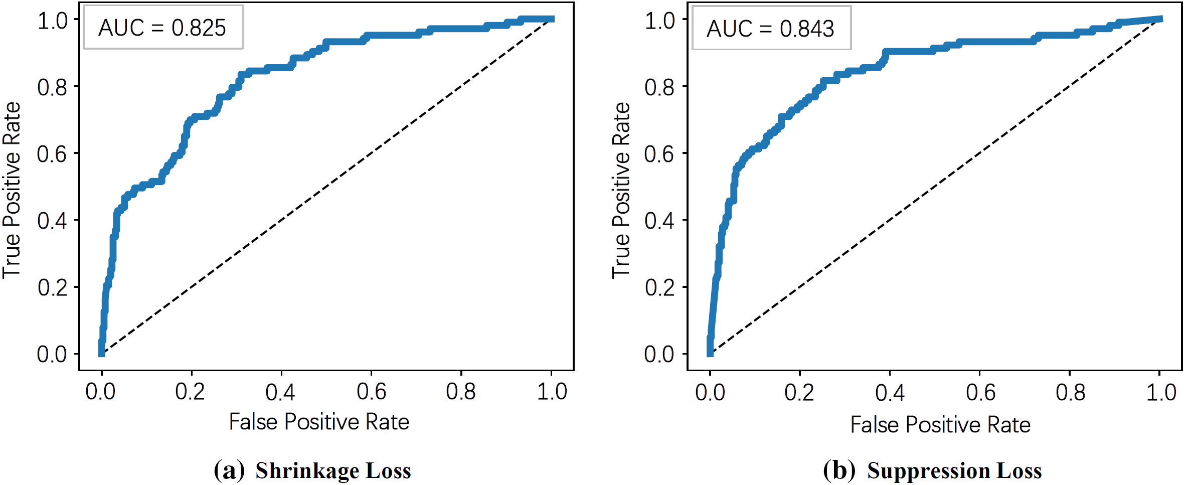
Figure A1: Receiver operating characteristic (ROC) curve of shrinkage and suppression loss. The ROC curve is generally used to reflect the threshold sensitivity and prediction accuracy of a model. The value of AUC represents the area under the ROC curve. The larger the area the better the prediction effect. We can see that the AUC value of the suppression loss is greater than that of shrinkage, indicating that suppression loss has better predictive performance

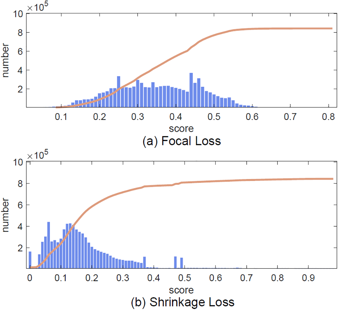
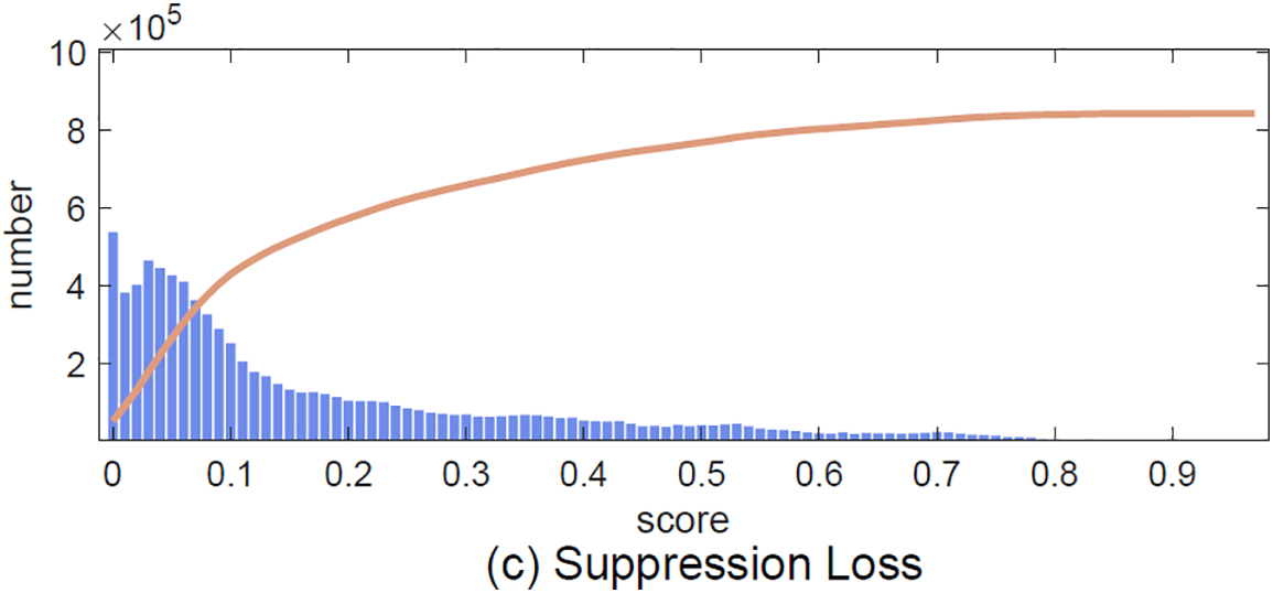
Figure A2: Distribution of predicted score by shrinkage loss and suppression loss. In the scoring process, we hope that the scores are concentrated at both ends, i.e., there are many sample points with low and high scores, but the scores are relatively small. A more concentrated number of scores, at a certain value (such as (a)), means that the algorithm does not distinguish the scores. It demonstrates that suppression loss is better than shrinkage loss and focal loss in classification performance